Mass Balance Evolution of Black Rapids Glacier, Alaska, 1980–2100, and Its Implications for Surge Recurrence

1. Introduction

Of the ~200,000 glaciers worldwide (Pfeffer et al., 2014), >2,300 have been identified as surge-type glaciers (Sevestre and Benn, 2015). A large fraction thereof, >300 surge-type glaciers, lie in Alaska and neighboring Canada. Over the last decades, this region has been subject to strong warming (e.g., Bieniek et al., 2014), which is the main driver for the dramatic observed glacier mass losses (Arendt et al., 2009). Due to their unique dynamic behavior, surge-type glaciers complicate both observational (e.g., Larsen et al., 2015) and modeling studies (e.g., Radić et al., 2014) that aim to constrain their response to warming. This provides an incentive for improved observation and modeling of surge-type glaciers.

In this paper, we focus on Black Rapids Glacier, a surge-type glacier in interior Alaska that last surged in 1936–1937. While Black Rapids' surge reservoir experienced a net elevation gain from ~1950 to 1995 (Shugar et al., 2010), no net gain was observed over the period 1980–2010 (Kienholz et al., 2016), likely due to the warming atmosphere. Workers on other surge-type glaciers in the Alaska-Yukon region found that climate change prolonged surge recurrence intervals and/or attenuated surge magnitudes (Eisen et al., 2001; Flowers et al., 2011; Bevington and Copland, 2014). In the case of Black Rapids Glacier, Kienholz et al. (2016) hypothesized that a surge in the near future is unlikely.

Here we employ a mass balance model to reconstruct Black Rapids' mass balance for the period 1980–2015 and to project it for the period 2015–2100. Our goal is to assess the evolution of Black Rapids Glacier with an extra focus on its surge likelihood. To model the surface mass balance, we use a distributed enhanced temperature index melt model forced with temperature and precipitation fields downscaled from the ERA-Interim reanalysis (Dee et al., 2011) and calibrated with an extensive and previously unused set of field measurements. A retreat parametrization and a simple debris model are applied to account for glacier geometry changes and the effects of changing debris extent. Uncertainties are quantified systematically using a Monte Carlo approach, which improves on the widely used approach of choosing one single optimal input/parameter combination.

2. Study Site

Black Rapids Glacier is a surge-type valley glacier located in the western portion of the Eastern Alaska Range known as the Hayes Range (Figure 1A). In 2010, Black Rapids was 41.3 km long and occupied an area of 241.5 km², 44.5 km² (18.5%) of which were covered by moraine and rockslide debris (Figure 1B). The extensive rockslide debris (~11 km²) was deposited during the M 7.9 Denali Fault earthquake in November 2002.

FIGURE 1

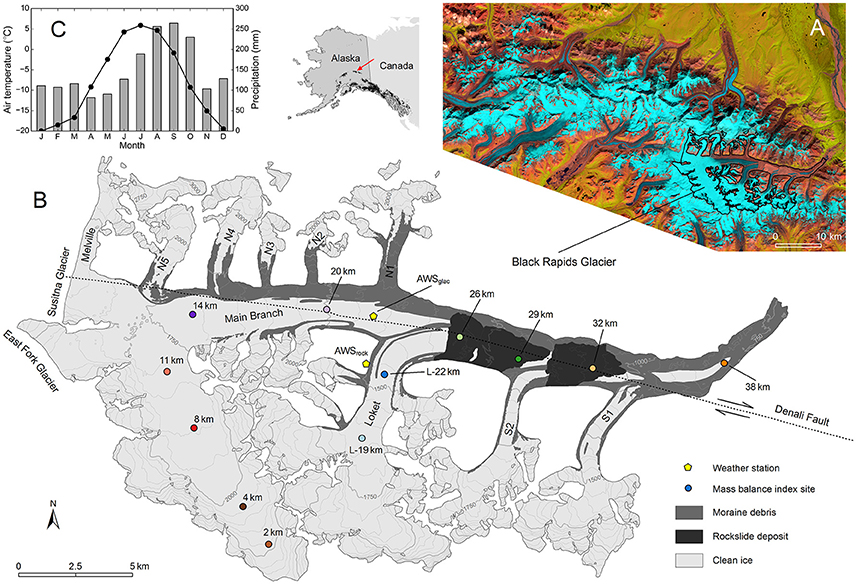
Figure 1. (A) Landsat Operational Land Imager (OLI) false color composite from July 13, 2013, showing Black Rapids Glacier along with the glaciers of the Hayes Range (western part of the Eastern Alaska Range). (B) Map of Black Rapids Glacier with glacier extent, surface topography, debris cover and rockslide deposits for the year 2010. The approximate location of the Denali Fault, the locations of the mass balance index sites and the automatic weather stations (years 2012–2014) are also shown. (C) Monthly mean temperatures (dotted line) and total precipitation (bars) based on the Parameter-elevation Relationships on Independent Slopes Model (PRISM) climatology (Daly et al., 1994). The diagram was derived by averaging temperature and precipitation from all the PRISM grid points within Black Rapids' perimeter (62 points).

Black Rapids Glacier currently ranges from ~700 to 3,650 m a.s.l., with its median elevation at ~1,850 m. It has three southern and six smaller northern tributaries, and shares two major divides with the Susitna and East Fork Glaciers. Black Rapids is part of Alaska's Southeast Interior climate zone (Bieniek et al., 2012), where high latitude and marked continentality cause long cold accumulation and short warm ablation seasons. Only 3 months per year have glacier-wide mean temperatures above freezing (Figure 1C). Monthly mean precipitation is typically ~100 mm, but reaches ~250 mm during fall (August–October).

During its last surge in 1936–1937, Black Rapids reached a length of ~46.5 km. Over the recent decades, the glacier has been subject to considerable thinning and retreat. From 1980 to 2010, its length and area decreased from 42.7 to 41.3 km (–1.4 km) and 248.8 to 241.5 km² (–7.3 km²), respectively (Kienholz et al., 2016). The corresponding specific mass balance was –0.48 ± 0.07 m w.e. a^–1 for the entire period, and more negative for the period 2001–2010 (–0.64 ± 0.11 m w.e. a^–1) than the period 1980–2001 (–0.42 ± 0.11 m w.e. a^–1).

Black Rapids Glacier has been studied extensively over the past decades (see Kienholz et al. (2016) for a summary of the previous work). A surface mass balance monitoring program was initiated in 1972 by the U.S. Geological Survey (USGS), the University of Alaska Fairbanks and the University of Washington (Heinrichs et al., 1995). This ongoing program has resulted in extensive point observations (Heinrichs et al., 1995; Truffer et al., 2005), placing Black Rapids Glacier among Alaska's glaciers with most surface mass balance measurements. So far, however, these point observations have not been used to estimate glacier-wide mass balances or for mass-balance modeling applications.

3. Data

For the forcing of the mass balance model, we used dynamically downscaled daily ERA-Interim temperature and precipitation fields for the hindcasting period 1980–2015. Quantile mapped versions of these fields matching the GFDL-CM3 RCP 8.5 climate scenario, as well as a constant climate scenario, were used for the forecasting period 2015–2100. For calibration and validation of the surface mass balance model, we used in situ surface mass balance observations (point balances), geodetic mass balances and snow line elevations derived from satellite imagery. Glacier topography and ice thickness were taken from digital elevation models (DEMs) and a global ice thickness dataset, respectively. The glacier extent and debris-cover input for the model were mapped from aerial and satellite imagery.

3.1. Outlines and DEMs

Outlines derived from high resolution aerial imagery [Alaska High Altitude Aerial Photography (AHAP), Brooks, 1988] and satellite imagery (IKONOS and Worldview-2, © 2011, DigitalGlobe, Inc.) were available for the years 1980, 2001, and 2010, enclosing glacier areas of 248.8, 243.1, and 241.5 km², respectively (Kienholz et al., 2016). For the same years, we had DEMs available. Most applications in this study relied on the 2010 DEM, which was derived from airborne InSAR (X-band) through interferometry (http://ifsar.gina.alaska.edu). This DEM has a native resolution of 5 m and a vertical precision of ~1 m.

Calibration of our surface mass balance model required annually updated outlines and DEMs (Section 4.4). We prepared the DEM time series by linearly interpolating elevation changes between the DEMs available. For the outlines we chose a similar approach and linearly interpolated horizontal rates of change between the outlines available. Though this approach oversimplifies the true signal, it is closest to reality in the absence of additional observations. Note that Black Rapids' terminus is heavily debris-covered, making frequent outline updates based on satellite imagery challenging.

3.2. Ice Thicknesses/Glacier Bed

Ice thicknesses were extracted from a global dataset computed by Huss and Farinotti (2012). Their approach employs a parametrized surface mass balance gradient (adjusted for surface elevation change) to determine the volumetric balance flux along a glacier's elevation profile. Employing Glen's flow law and a sliding parametrization, they solve the balance flux for an average ice thickness at each elevation band. Using slope and distance to the glacier margin (derived from DEM and glacier outlines), they finally compute spatially distributed ice thicknesses from the longitudinal thickness profile.

For Black Rapids Glacier, Huss and Farinotti (2012) used a DEM from 2010 (identical to the 2010 InSAR DEM used in this study) and outlines compiled by Kienholz et al. (2015). To match the improved outlines used here, we adapted the ice thicknesses manually, mostly along the glacier margins. The results modeled (for the year 2010) suggest a mean ice thickness of 205 m and a maximum ice thickness of 630 m. The total glacier volume is 49.6 km³.

We used previous ice thickness observations (Heinrichs et al., 1995; Gades, 1998) complemented by our own measurements to assess the uncertainties of the ice thickness map. Gades (1998) obtained ice thicknesses in 1993 by ground-based low-frequency radio echo sounding (5 MHz), covering 12 profiles in the upper glacier area (Figure S1). The thickness observations compiled in Heinrichs et al. (1995) were obtained by radio echo sounding also, however, they were taken mostly in spring 1990 and cover the lower part of the glacier. We conducted an additional radar survey in spring 2012, covering the lower part of the Loket tributary (Figure 1). The uncertainties of the radar-derived thicknesses arise from uncertainties in the wave speed (±0.5%) and the selection of the migrated bed reflection (±15 m, Gades, 1998). The uncertainties in the ice thicknesses from Heinrichs et al. (1995) are larger (±10%), as the radar data was not migrated (Heinrichs et al., 1995, 1996). To account for the glacier elevation changes between the dates of the radar surveys and 2010 (date of the DEM), we subtracted the measured ice thicknesses from the ice surface elevations recorded during the surveys. This yielded bed elevations, which we then subtracted from the 2010 ice surface elevations to obtain adjusted ice thicknesses. Erosional or tectonic changes to bed elevation were neglected due to lack of data.

Comparison of the modeled and measured thicknesses indicated a small bias (−12.3 m, modeled ice too thick) accompanied by larger scatter (100.0 m mean absolute error, Figures 2A,B). Evaluating individual profiles indicated that the model typically underestimated ice depths at the profile center while overestimating them closer to the margins. In the lowest glacier reaches, the modeled glacier bed is systematically shallower than suggested by measurements. The measured ice thicknesses typically lie within ±34% (1σ) of the modeled thicknesses (Figure 2C).

FIGURE 2

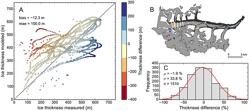
Figure 2. (A) Modeled vs. measured ice thickness with colors showing the thickness difference (measured—modeled). Blue shades (positive thickness differences) indicate that the modeled bed is too shallow. The measured thicknesses are adjusted for the 2010 surface. The map in (B) shows the thickness differences at their actual locations on the glacier, using the same colors as (A). (C) Frequency distribution of thickness differences (in percent of the modeled ice thickness), with the red line showing the Gaussian fit.

3.3. Debris Cover and Transient Snow Lines

We derived time series of debris cover and snow line elevations from medium-resolution Landsat spaceborne imagery (Thematic Mapper (TM), Enhanced Thematic Mapper (ETM+), Operational Land Imager (OLI)). While Landsat imagery has a limited spatial resolution of 30 (TM) and 15 m (pansharpened ETM+, OLI), one scene captures ~185 × 185 km in area, and thus Black Rapids Glacier in full (at the pass/row combinations 68/15, 68/16, and 67/16). The Landsat data was downloaded from the USGS EarthExplorer website (http://earthexplorer.usgs.gov).

3.3.1. Debris Cover

Using 12 Landsat summer images and one aerial orthomosaic (Table S1), we obtained a series of debris layers in a semi-automated fashion. With the band ratio of red and shortwave infrared thresholded at 1.6, we derived an initial debris layer from a 1987 Landsat TM image. We then adapted this layer manually to arrive at the debris mask of the remaining scenes. This allowed us to classify the debris into rockslide debris and moraine debris, two categories with different thicknesses on Black Rapids Glacier (Kienholz et al., 2016). The manual adaptation also allowed us to account for transient snow lines that fluctuated among images, sometimes obscuring debris portions at higher elevations. From 1980 to 2015, Black Rapids' debris cover increased by ~10 km² (from 35.4 to 45.4 km², Table S1), with a step change following the 2002 rockslides. The three 2002 rockslides buried ~11 km² of the glacier, of which ~5 km² were clean ice prior to the rockslides and ~6 km² covered by moraine debris.

For the mass balance model, we converted the 13 debris layers (spaced 1–7 years apart, Table S1) into an annual debris time series. Linear interpolation, as implemented for glacier outlines and DEMs, proved impractical for debris. For each year without a derived debris layer, we thus adopted the debris layer closest in time.

3.3.2. Snow Lines

Our transient snow line time series is based on 59 Landsat images taken between 1986 and 2015, but predominantly (50 scenes) after the year 2000. Tests indicated challenging conditions on Black Rapids Glacier for the automatic delineation of snow lines through band thresholding due to the steep, rough topography. To achieve the most accurate snow line elevations, we thus opted for a workflow that automated all the processing steps except for the actual snow line delineation (Supplementary Section 1). To estimate the accuracy of the derived snow lines, two operators derived two separate snow line datasets from the 59 Landsat scenes.

Rather than deriving one glacier-wide snow line elevation per Landsat scene, we treated the nine largest glacier branches individually. This resulted in more than 300 snow line elevations for the main branch, Loket branch, and branches S1–S2 and N1–N5 (Figure 1). The branch-specific snow line elevations allowed us to validate the model output on smaller spatial scales, which is desirable given that Black Rapids Glacier covers branches with opposing aspects and potentially different microclimates. Treating the branches individually also allowed us to take advantage of partly cloudy satellite scenes.

3.4. Mass Balance Data

3.4.1. Geodetic Mass Balances

Kienholz et al. (2016) calculated geodetic mass balances including uncertainties for the periods 1980–2001 and 2001–2010 based on a range of elevation products. For the present study, we also used a third, laser altimetry-derived geodetic mass balance, covering the period 1995–2000 (Larsen et al., 2015).

3.4.2. In situ Point Mass Balances

The mass balance monitoring program on Black Rapids Glacier focused on the main branch and the Loket tributary (Figure 1). The frequency of the visits, as well as number and location of the index sites, varied over the course of the program. From the mid 1970s to the mid 1980s, surface mass balances were measured at up to ten index sites covering most of Black Rapids' elevation range (Heinrichs et al., 1995, 1996). Up to eight index sites (all the sites in Figure 1, except for the more recent sites 11 and 29 km) were maintained along the centerline of the main glacier branch (between ~900 and 2,200 m a.s.l.) and two (L-22 and L-19 km) along the centerline of the Loket tributary (at ~1,500 and 1,650 m a.s.l.). The sites were visited at least twice a year in spring and fall, allowing for the derivation of seasonal mass balances.

The mass balance program was downsized in the latter half of the 1980s. Maintenance of several work-intensive index sites located very high and very low on the glacier (2, 4, 26, 32, 38, L-19 km) was suspended and the number of visits restricted to one spring visit typically. During the mid-1990s, two new index sites (11 and 29 km) were established, however, site 29 km was buried by the 2002 rockslide deposits and not reestablished thereafter. Over the last decade, the mass balance program has consisted of two to four sites (8, 14, 20, L-22 km) visited once per year in spring (Truffer et al., 2005). Two index sites, 8 and 14 km, have a nearly continuous record of annual mass balances over the length of the mass balance program (see Figure 11 in Kienholz et al., 2016).

For each index site, we derived mass balances from measured stake heights and snow depths along with densities of the material (ice, snow, firn) gained or lost. For the early period with at least two visits per index site per year (spring and fall, with intermittent summer visits), we derived the seasonal balances in the floating time system (Cogley et al., 2011). Winter balances for the later period (one spring visit only) were obtained in the combined time system (i.e., the accumulation from the stratigraphic surface of the previous year to the surface at the time of the spring visit), while the corresponding annual balances refer to the stratigraphic time system. To obtain error estimates for the point balances, we adopted procedures and error estimates outlined previously (Heinrichs et al., 1995, Supplementary Section 2). We transferred the final point balances, including error estimates, into a relational database from which they served the mass balance model and other applications.

3.5. Climate Data

3.5.1. Reanalysis Data

The atmospheric forcing for the ~37 year hindcasting period January 3, 1979 to October 29, 2015 was provided by Bieniek et al. (2016). They applied the Weather Research and Forecasting (WRF) Advanced Research core (Skamarock et al., 2008) to dynamically downscale the ERA-Interim reanalysis (Dee et al., 2011) from ~100 to 20 km spatial resolution. To force our mass balance model, we used near-surface (2 m) temperature means and precipitation sums at daily time steps, which we derived from the hourly WRF output.

3.5.2. Future Scenarios

For the ~85 year forecasting period October 30, 2015 to December 31, 2100, we worked with two forcing scenarios, a lower bound constant climate scenario and an upper bound RCP 8.5 scenario. The RCP 8.5 scenario projects a warming of ~6.5°C between 2015 and 2100 and a corresponding precipitation increase of ~30% relative to the 2015 value. This scenario was provided by Lader et al. (submitted), who downscaled both the historical run and the RCP 8.5 scenario from the Geophysical Fluid Dynamics Laboratory Climate Model version 3 (GFDL-CM3, Donner et al., 2011). Employing a quantile-mapping algorithm (e.g., Cannon et al., 2015), they determined the temperature and precipitation differences between the future and historical GFDL runs, and used these differences to adjust the WRF-downscaled ERA-Interim reanalysis from Bieniek et al. (2016), which served as the observational dataset. Using 30 years of ERA-Interim data (1981–2010), they produced adjusted climate data with preserved short-term variability for the time periods 2011–2040, 2041–2070, and 2071–2100. Rather than employing their full 2011–2100 time series, we used the reanalysis data from Bieniek et al. (2016) until the overlap of the two series ended on October 29, 2015. For the constant climate scenario, we repeated the same 30 year period (1981–2010) without adjusting temperatures and precipitation. Figure 3 illustrates the three time series used for the atmospheric forcing.

FIGURE 3

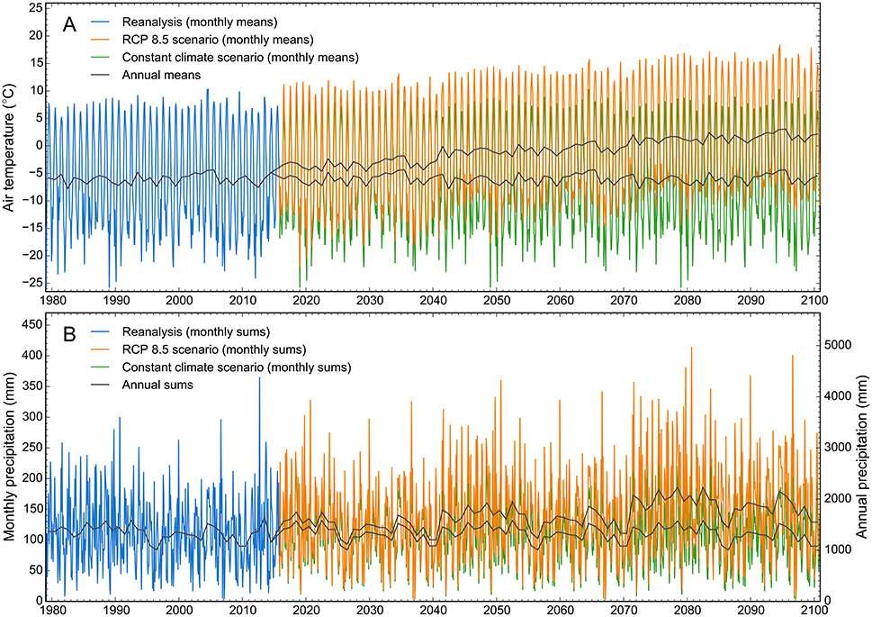
Figure 3. (A) Near-surface air temperature and (B) precipitation time series taken from the WRF-downscaled ERA-Interim reanalysis (January 3, 1979 to October 29, 2015, used for hindcast) and the two forecast scenarios RCP 8.5 and constant climate (October 30, 2015 to December 31, 2100). The data are taken from the WRF gridpoint with center at 63.42°N and 146.18°W and an elevation of 1,525 m a.s.l.

The downscaled versions of the RCP scenarios 2.6, 4.5, and 6.0 were unavailable at the time of this study, preventing us from using them in our modeling efforts. The corresponding projections lie within those from our two scenarios, as each of the three scenarios assumes a slower increase in greenhouse gas emissions than RCP 8.5 does. Although the RCP 8.5 scenario projects rapidly increasing greenhouse gas emissions and thus infers substantial radiative forcing (8.5 W m^–2, Riahi et al., 2011), it may be more likely to occur than the constant climate scenario, in light of the recent evolution of greenhouse gas emissions (Sanford et al., 2014).

3.5.3. Downscaling

The WRF-downscaled climate products (both reanalysis data and future scenarios) come with a spatial resolution of 20 km, considerably coarser than the 100 m resolution of our glacier model. The elevation differences between the 20 km DEM of the WRF-model and the DEM of our glacier model reach several 100 m (Figure 4), demanding additional downscaling steps. We took a simple approach similar to that of previous workers (e.g., Machguth et al., 2009; Schaefer et al., 2013). Assuming that the WRF-modeled temperature and precipitation reflect the center of each 20 km cell, we interpolated among cells, accounting for the topography using temperature lapse rates and precipitation gradients. In practice, we applied a three step procedure. For the temperatures, we brought the 20 km values (T^20km) to sea level ($T_{0m}^{20km}$), applying the lapse rate l to the WRF topography (z^20km):

$\begin{array}{rc}{T}_{0m}^{20km}=T^{20km}+z^{20km}/l& (1)\end{array}$

FIGURE 4

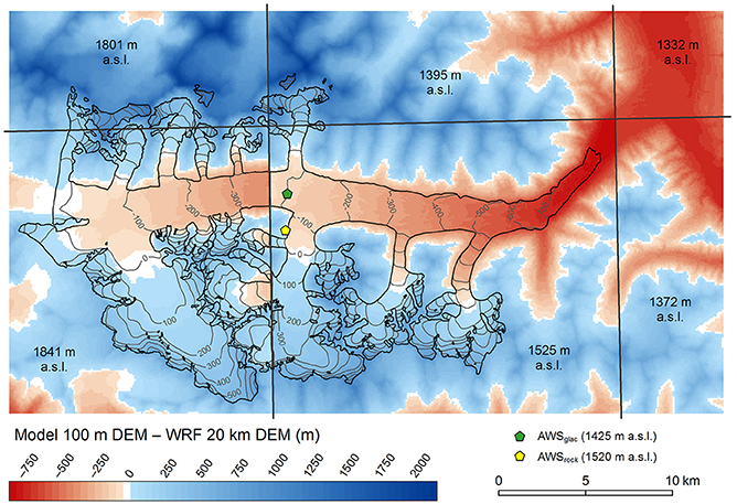
Figure 4. Elevation difference between the 100 m DEM used for the glacier modeling (year 2010) and the 20 km DEM used to dynamically downscale the ERA-Interim data. Elevation differences exceed 1,000 m in the highest and −700 m in the lowest glacier reaches. The edges of the 20 km DEM cells are indicated with black lines and the cell elevations are annotated. Within the glacier perimeter, 100 m contours of the elevation differences are given for reference. Prior to the differencing, the 20 km DEM was resampled to 100 m. AWS_glac and AWS_rock mark the locations of the two weather stations.

We then bilinearly interpolated $T_{0m}^{20km}$ to the 100 m grid ($T_{0m}^{100m}$) and computed temperatures for each grid cell of the 100 m DEM (z^100m) by applying the same lapse rate in reverse:

$\begin{array}{rc}{T}^{100m}=T_{0m}^{100m}-z^{100m}/l& (2)\end{array}$

The processing for precipitation was similar. We first brought the 20 km precipitation (P^20km) to a reference elevation of 1,500 m a.s.l. ($P_{1,500m}^{20km}$) using the precipitation gradient s:

$\begin{array}{rc}{P}_{1,500m}^{20km}=P^{20km}/(1+(z^{20km}-1,500)·s)& (3)\end{array}$

We then bilinearly interpolated the precipitation to a 100 m grid ($P_{1,500m}^{100m}$) and reintroduced topographic effects by applying s to z^100m:

$\begin{array}{rc}{P}^{100m}=P_{1,500m}^{100m}·(1+(z^{100m}-1,500)·s)& (4)\end{array}$

Precipitation gradients are tied to a reference elevation, which defines the reference (100%) precipitation. With multiple distributed precipitation values at different elevations (defined by the WRF topography), we specified one reference elevation to ensure the same gradient was employed across the modeling domain. While this elevation can be chosen randomly (we used 1,500 m a.s.l.), the optimized gradient in the mass balance model will vary as a function of the reference elevation chosen.

While the precipitation gradient s is a calibration parameter of the mass balance model (Section 4.1), we derived the temperature lapse rates from the WRF near-surface temperatures directly. Over weekly periods, we combined the temperature-elevation pairs of the 12 WRF cells in the Black Rapids domain, and then estimated the lapse rates using linear regression. As expected, the lapse rates are lowest in winter and highest in spring. Throughout the melt season, they vary between 6.0 and 7.2°C km⁻¹.

During the calibration of the mass balance model (Section 4.4), we used our DEM time series (Section 3.1) to annually update the 100 m topography z^100m employed during the downscaling. During the final hindcast and projection runs (Sections 5.1, 5.2), we used the updated DEMs produced by our model instead.

3.5.4. Bias Check

We used in situ air temperature observations taken during the summers of 2012–2014 to evaluate potential biases in the WRF near-surface temperatures. Air temperatures were measured both off-ice and on-ice at the locations AWS_rock and AWS_glac, at 1,520 and ~1,425 m a.s.l., respectively. The deployed Vaisala temperature sensors recorded near-surface temperatures (~2 m above ground) at sub-hourly time steps (varying between 10 and 15 min over the three seasons), which we averaged to match the daily resolution of the WRF data.

Overall, the daily averaged in situ temperatures agree well with the corresponding WRF temperatures. The off-ice comparison suggested very small warm biases (< 0.5°C) in the WRF temperatures throughout the three seasons (Figure 5A), which we considered too small to justify a correction of the WRF input across the glacier domain. The temperatures at the on-ice station were several degrees colder than the WRF output during the melt season, while they matched well during times without melt (Figure 5B). During the melt season, the near-surface air cools by transferring heat to the ice (which cannot exceed 0°C), a process not reproduced in the WRF model due to its coarse resolution (glacier ice is not represented in the WRF surface grid). Temperature index models have been shown to perform better when forced by off-ice temperatures (Lang, 1968), hence we refrained from correcting this seasonal difference in the WRF data prior to the calibration. During model calibration, the choice of appropriate melt and radiation factors accounts for the difference indirectly.

FIGURE 5

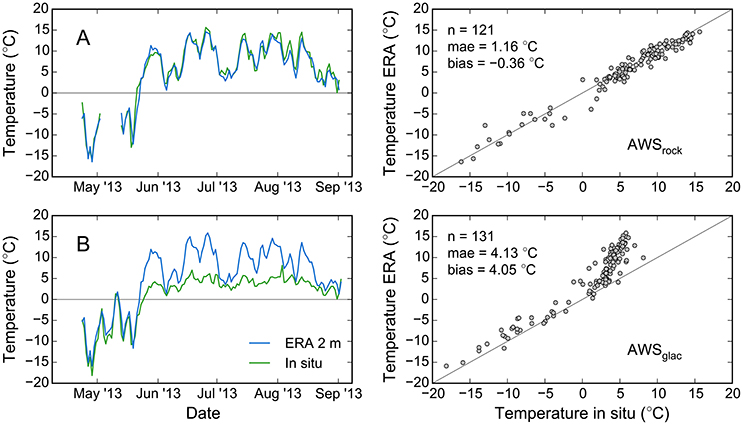
Figure 5. Daily average in situ air temperatures vs. downscaled ERA-Interim near-surface (2 m) temperatures for (A) the off-ice station AWS_rock and (B) the on-ice station AWS_glac (Figure 1) during the 2013 season. Results are similar for the 2012 and 2014 season. The off-ice station had a measurement gap in May 2013.

4. Glacier Model

For the modeling of the glacier mass balance, we implemented an enhanced temperature index melt model coupled to a simple elevation-dependent accumulation model. To consider the melt reduction under debris, we added a simplified model that accounts for the evolution of moraine debris and the advection of rockslide debris. To account for the glacier's geometry changes, we implemented a retreat model. For the mass balance model calibration, we developed code that can leverage all types of calibration data including geodetic balances, snow line elevations, and point mass balances, with the latter in all possible time systems. Advancing the calibration included establishing communication with a relational database hosting calibration data and other model input.

4.1. Surface Mass Balance

Following Hock (1999), we implemented an enhanced temperature index model, which runs in a distributed fashion on a 100 m grid, and at daily time steps. The chosen spatial and temporal resolution is a compromise between desired level of spatial/temporal detail and required computation time. Given the model's use for Monte Carlo simulations, computation time was critical.

Melt, M (mm d^–1), is derived from daily average air temperature, T (°C), by

$\begin{array}{ll}M=\{\begin{array}{cc}(f_m+r_{snow/ice}·I)·T·d\hfill & :T>0\hfill \\ 0\hfill & :T<0\hfill \end{array},\hfill & (5)\end{array}$

where f_m is the melt factor (mm d⁻¹ °C⁻¹), r_snow/ice are the radiation factor of snow and ice (mm m² W⁻¹ °C⁻¹ d⁻¹), and I is the potential clear-sky direct solar radiation (W m⁻²). When firn is exposed at the glacier surface, the radiation factors of snow, r_snow, applies. While f_m and r_snow/ice are calibration parameters, I is calculated from the DEM using standard algorithms. T is the near-surface air temperature as downscaled from the WRF data (Section 3.5.3). The melt reduction factor d equals 1 (no reduction) in debris-free areas (ice, snow, firn). In debris-covered areas, d = 1 if snow > 0.1 m w.e. covers the debris. Between 0.1 m w.e. snow cover and snow-free conditions, d increases linearly from 1 to 5 to account for the accelerated snow melt above the debris surface. Once all the snow has melted and the debris is exposed, melt is reduced (d < 1). We assume d = 0.05 (95% melt reduction compared to debris-free conditions) for the several meter thick rockslide debris, based on sparse field observations that show minimal ice melt below the debris (D. Shugar, personal communication, 2016). For moraine debris, d is obtained from the calibration (Section 4.4).

To model snow accumulation, the solid part of the precipitation is retained, while the liquid part is assumed to run off without refreezing. A smooth transition between solid and liquid precipitation is obtained by applying a linear function between 0.5 and 2.0°C. Beyond these thresholds, the retained solid precipitation is 100 and 0%, respectively. The accumulation model has two calibration parameters, the precipitation gradient s (used during the precipitation downscaling, Section 3.5.3) and a precipitation factor p, which acts as a glacier-wide multiplier for the downscaled precipitation field.

At the end of each calendar year, the winter and summer surfaces of that year are determined by analyzing the cumulative mass balance grids. Detecting the seasonal surfaces allows for modeling mass balances in the stratigraphic and combined time systems, which is required to take full advantage of our calibration data. To be able to track the transient snow lines in the model, we distinguish snow from firn. Every year, snow older than the previous summer surface is added to the firn, which is treated crudely in our model: firn is retained for 7 years or until the firn layer exceeds 10 m w.e. in thickness. To obtain realistic snow and firn thicknesses at the beginning of the modeling period, the mass balance model is run repeatedly for the first year before the actual run is launched.

4.2. Glacier Geometry

A simple retreat model based on the mass conserving Δh-parametrization by Huss et al. (2010) is applied to account for glacier geometry changes. The parametrization prescribes the relationship between ice thickness change (Δh) and elevation based on observations rather than application of an actual ice flow model. Compared to a flow model, the Δh-parametrization has low computational costs and requires no calibration in the typical sense (prescription of the glacier-specific Δh-curve is sufficient). We derived Black Rapids' Δh-curve from centerline elevation changes measured between 1995 laser altimetry profiles and the 2010 InSAR DEM (Kienholz et al., 2016), excluding the areas affected by the 2002 rockslide deposits. Including these areas in the Δh-curve would be misleading: upon glacier retreat (and normalization of the curve with a smaller elevation range), the rockslides' reduced thinning signal would be applied outside the actual rockslide debris.

The Δh-parametrization is coupled to the surface mass balance model and run on annual time steps, yielding updated surface elevations and glacier extents each year. Mass conservation is checked for every iteration. Following Huss et al. (2010), surface lowering is restricted not to exceed that year's most negative surface mass balance in ice equivalent; moreover, the Δh-parametrization is not applied in areas where ice thickness is less than 10 m. For the few years with positive glacier-wide mass balances, the excess mass is distributed evenly across the glacier, not allowing for glacier advance. To account for the rockslide debris, we exclude the rockslide areas from the Δh-parametrization and apply only the surface mass balance field across those areas. This approach preserves the ice under the rockslide debris more realistically than the original Δh-parametrization, although it neglects flux divergence under the debris. Neglecting flux divergence most likely leads to missed emergent flow early in the modeling period and missed submergent flow later on (the increasing elevation difference between the rockslide deposits and neighboring clean ice causes the switch from emergent to submergent flow). Shugar et al. (2012) describe a more sophisticated approach that considers flux divergence under Black Rapids' rockslide deposits, however, this model is too computationally expensive for our Monte Carlo simulations.

The Δh-parametrization is generally well suited for glaciers with negative mass balances and thus retreat. It is less ideal for glaciers with positive mass balances and, due to its parametrized nature, unable to model an actual surge. Given that Black Rapids Glacier has not shown thickening over the past decades (and thus no buildup toward a next surge), we consider application of the Δh-parametrization appropriate to model Black Rapids' future evolution. To assess the likelihood of a surge, we apply an alternative approach calculating elevation changes at the index sites based on measured emergence velocities and modeled mass balances (Section 5.3).

4.3. Debris

Our simple debris model runs on annual time steps and treats rockslide debris and moraine debris separately. While it adapts the extent of the debris layers, it does not capture thickness changes and neglects mass conservation in general. Rockslide debris is translated downglacier based on an idealized ice flow velocity field. The rockslide margins are intersected with the velocity field and moved as prescribed by directions and speeds from the intersected velocities. Without an ice flow model and complete velocity fields from satellite data, we interpolated ice flow directions from flow lines digitized on Landsat imagery. For simplicity, the speeds were approximated by parabolas (binary logarithm of the glacier cell's distances to the closest margin) and multiplied by a tuning factor (0.54) to match 42 annual speeds derived by manual feature tracking on a pair of Landsat images (from 2003 and 2015, respectively).

The evolution of the moraine debris relies on a prescribed relationship between normalized elevation range and moraine debris-cover fraction. Each year, considering the topography changes from the retreat model, the moraine debris layer is updated to meet the prescribed debris fraction for each elevation bin. To achieve lateral debris growth, ice cells are converted to moraine debris along the boundaries of the existing moraine debris layer. Removal of moraine debris is not allowed, which is consistent with the predominant glacier retreat. We derived the Black Rapids-specific relationship between elevation range and moraine debris fraction from the debris layer for the year 2015 (Section 3.3.1) using 100 m elevation bins.

4.4. Mass Balance Model Calibration and Validation

We calibrated six parameters for the surface mass balance model: two for the accumulation model (s, p) and four for the melt model (f_m, r_snow, r_ice, d). The goal of the calibration was to maximize the agreement between modeled and observed point mass balances as well as modeled and observed glacier-wide (geodetic) mass balances. The calibration period comprised the mass-balance years 1980–2013. Validation of the surface mass balance model was based on Landsat-derived snow line elevations.

Throughout the calibration, glacier extent, surface elevation and debris cover were prescribed from observations, in order to capture three important feedback mechanisms (e.g., Elsberg et al., 2001): (1) the positive climate-elevation feedback, (2) the negative feedback due to glacier retreat, and (3) the negative feedback due to increasing debris cover. The three feedbacks affect the geodetic balances, and in the case of the climate-elevation feedback also the in situ mass balance measurements (due to the elevation lowering of the index sites).

4.4.1. Calibration

Following Trüssel et al. (2015), we searched the parameter space systematically within prescribed ranges, which is a simple, yet computationally intense process. To reduce the computational costs, we split the calibration into two steps. In the first step, we constrained a plausible range of precipitation factors and gradients based on our set of observed winter point mass balances. In the second step, we used both seasonal and annual point mass balances, as well as geodetic balances, to fine-tune the precipitation factors/gradients and to calibrate the four parameters of the melt model. To ensure independence of the seasonal and annual mass balances in the second step of the calibration, we relied on seasonal balances before 1989 and annual balances thereafter (Figure S2). Our grid search across the parameter space resulted in >150,000 model runs.

Rather than deriving one single best parameter combination for further analysis, as often done in previous studies, we determined a range of best parameter combinations which we all considered equally valid. We chose them as follows. First, we compared the modeled glacier-wide mass changes to the three geodetic mass balances (available for the periods 1980–2001, 2001–2010, and 1995–2000, Section 3.4.1), and extracted all parameter combinations that yielded balances within the uncertainties of the observations for all three periods. This resulted in 4,576 combinations, which we further reduced by considering the agreement between modeled and observed seasonal and annual point mass balances. To account for the uncertainties in the point balances (Section 3.4.2) we randomly varied the measured point balances within their errors 10,000 times. Each time, we recalculated the mean absolute error (mae) of the modeled balances for each parameter combination and gave the solution with the lowest mae the first rank. Solutions that achieved the first rank at least once (40 solutions) were then kept as the best solutions (Figure 6, Figure S3). Figure 7 illustrates the parameter values of those best solutions.

FIGURE 6

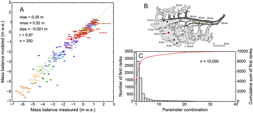
Figure 6. (A) Modeled vs. measured point mass balances for one of the 40 best parameter combinations modeled (f_m = 0.9, r_snow = 0.017, r_ice = 0.035, s = 12.4, p = 1.12, d = 0.45). Error bars indicate the uncertainties in the measured mass balances. Colors distinguish index sites with locations shown in map (B). The mass balances at the index sites 26, 29, and 32 km were observed before the deposition of the rockslide deposits. (C) Histogram indicating the number of first ranks accumulated during 10,000 model runs. The parameter combinations are numbered and ordered by the number of first ranks.

FIGURE 7

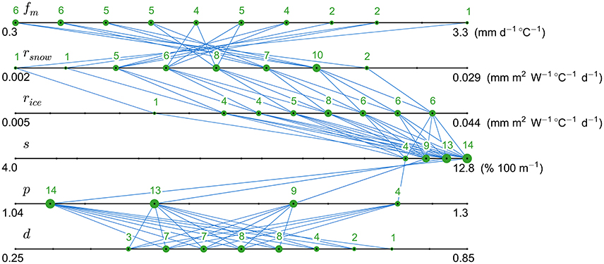
Figure 7. Parameter combinations of the 40 best calibration runs superimposed on the searched parameter space. f_m is the melt factor, r_snow/ice are the radiation factors of snow and ice, s is the precipitation gradient, and p and d are the precipitation and moraine debris melt reduction factors. Numbers on the left and right sides indicate the end members of the parameter space, including units. Small black dots on the lines show the parameter values tested. Blue lines connect the successful parameter combinations. The green points and their annotations indicate the number of successful combinations crossing through a particular parameter value. Precipitation gradients >12.8% 100 m^–1 caused implausibly low precipitation at the glacier terminus and thus were not accepted.

4.4.2. Validation

Given the simplicity of the model applied, observed and modeled snow lines matched well. Glacier wide, we found positive biases of 30–60 m when comparing the modeled snow line elevations from the best 40 parameter combinations to the Landsat-derived snow line elevations. The mean absolute error across all branches was typically ~100 m. Investigation of individual branches showed that the modeled snow lines of the north- and south-facing branches had opposite biases: in the south-facing branches, they were too low, while in the north-facing branches, they were too high (Figures 8A,B). Along the main branch, modeled and observed snow lines matched relatively well. Figure 8C illustrates the spatially varying mismatch using an example from August 2005. The biases found are unlikely due to errors in the Landsat-derived snow lines, although the derivation of snow lines from satellite imagery can be ambiguous. The comparison of the two independently derived snow line elevation datasets indicated considerable scatter (37 m mae) and a systematic difference (30 m bias), however the biases among the branches did not match the pattern emerging in the model-observation comparison (Figure S4).

FIGURE 8

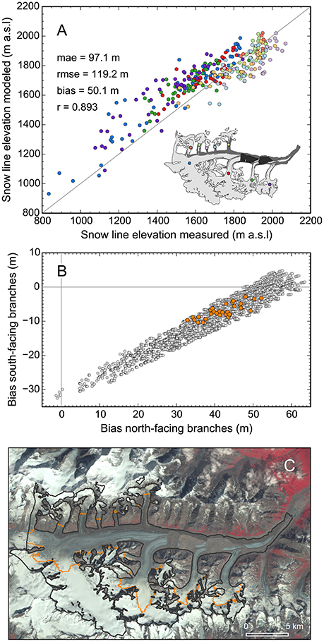
Figure 8. (A) Modeled vs. measured snow line elevations for the same parameter combination shown in Figure 6A. Among the 40 best parameter combinations, the solution shown has a relatively poor match with the measured snow lines. The color code in the inset map distinguishes individual branches. (B) Biases across the south-facing branches vs. biases across the north-facing branches for the 4,576 parameter combinations matching the three geodetic mass balances (gray points) and the 40 final parameter combinations (orange points). Ten final parameter combinations have identical biases, as the combinations differ only in the moraine debris melt reduction factor (d), which does not affect the snow line elevations. (C) Modeled snow lines (orange lines) vs. observation (Landsat Thematic Mapper (TM) composite) for August 8, 2005, illustrating that modeled snow lines are too high in the north facing branches and too low in the south facing branches.

None of the radiation/melt factor combinations of the 4,576 parameter combinations matching the geodetic balances eliminated the difference between north- and south-facing branches (Figure 8B). This indicates the biases are related to the modeled snow accumulation, which likely suffers from the use of spatially coarse precipitation input and our first-order downscaling approach. Our downscaling crudely represents orographic precipitation and neglects snow redistribution by avalanches and wind, the latter of which is important on Black Rapids Glacier. Snow redistribution by wind is challenging to model at present and often, redistribution grids based on observations are employed instead (e.g., Sold et al., 2013). However, our current observations at the index sites are too sparse to derive a glacier-wide snow redistribution grid, obliging us to accept the bias as-is for the present study. Future work may apply backward modeling of melt (e.g., Hulth et al., 2013) along the Landsat-derived snow lines to derive more spatially distributed end-of-winter accumulation data.

4.5. Monte Carlo Runs

Following the surface mass balance model calibration, we ran the glacier model over the full period covered by the climate data (January 1979–December 2100). While we prescribed the debris cover during the hindcasting period based on observations, we used the debris model to evolve the debris cover during the forecasting period. The retreat model was applied over the entire period. The model runs were set up separately for the two climate scenarios and conducted in a Monte Carlo fashion to explore uncertainties in the model results given the range of plausible model input parameters. The two scenarios provide a higher and a lower bound of possible glacier evolution including uncertainties.

Over the hindcasting period, we accounted for two sources of uncertainty, emerging from the choices of (1) mass balance model parameter combinations and (2) average density of the material gained/lost (prescribed during application of the retreat model). Each Monte Carlo run, we sampled from the 40 plausible mass balance model parameter combinations obtained during calibration and from a density range of 850 ± 60 kg m^–3. The same density range was applied for the derivation of the geodetic mass balances (Kienholz et al., 2016). To revert the modeled mass change into a volume change during the application of the retreat model, we reapplied the 850 ± 60 kg m^–3 density range for consistency reasons, and refrained from using the mass balance model to constrain the density of the material more precisely.

For the forecasting period, we considered additional sources of uncertainty, emerging from the uncertainty in (3) glacier bed elevation (ice thickness), (4) choice of the Δh-curve (prescribed during the retreat parametrization) and (5) choice of the debris evolution scenario (prescribed during the application of the debris model). Over the hindcasting period, (3)–(5) are observable and thus not considered sources of uncertainty. Regarding (3), we analyzed the match between modeled and measured ice thicknesses (Figure 2) and ultimately varied the ice thicknesses within ±34% of the values modeled by Huss and Farinotti (2012). This value corresponds to the standard deviation of the thickness difference distribution (Figure 2C). Each Monte Carlo run, one value was sampled from the ±34% range and applied systematically across the bed. We note this approach does not fully capture the complex mismatch pattern observed, which shows local mismatches beyond ±34%, but spatial autocorrelation smaller than the glacier's dimensions (Figures 2B,C). For (4), we first defined potential ranges for the Δh-curves (Figures S5A,B), informed by Δh-curves from previous studies (e.g., Huss et al., 2010). From this range, we sampled one curve per Monte Carlo run, which provided the Δh-curve for the year 2100. By linearly interpolating between the 2015 and 2100 Δh-curves, we obtained a smooth transition over time. For the constant climate scenario, we chose the plausible ranges more conservatively than for the RCP 8.5 scenario, as less marked climate/geometry changes occur in this case. Uncertainty source (5) was addressed similarly. First, we defined plausible ranges for the future moraine debris evolution (Figures S5C,D). Each Monte Carlo run, we sampled a debris curve from this range and interpolated between the observed curve from 2015 and the sampled curve. Typical debris curve shapes from the Alaska inventory (Kienholz et al., 2015) informed the definition of our ranges. Like above, plausible debris ranges were chosen more conservatively for the constant climate scenario. For the advection of the rockslide debris, we projected current velocities in the case of the constant climate scenario while implementing slowing speeds in the case of the RCP 8.5 scenario (linear slowing until 2050 and stagnant ice thereafter). The densities of the gained/lost material (uncertainty source 2) were kept as sampled during the hindcasting period in the case of the constant climate scenario. For the RCP 8.5 scenario, the sampled densities were adapted linearly to approach 900 kg m⁻³ in 2100, in order to account for the firn losses. Ultimately, we conducted 400 Monte Carlo runs for both climate scenarios, and derived means and standard deviations for each quantity of interest (e.g., area and mass changes). We retained the sampled parameters in order to run experiments (e.g., conventional vs. reference surface experiments) with identical parameters.

Although we considered key uncertainty factors in our Monte Carlo simulations, not all sources of uncertainty are included. With the strong warming predicted under the RCP 8.5 scenario, for example, partitioning of the energy budget may change significantly, questioning the validity of our mass balance model parameter combinations longer term. Estimating the future evolution of the parameter combinations is not feasible, forcing us to use the 40 parameter combinations calibrated over the hindcasting period.

5. Results and Discussion

5.1. Hindcasting

Over the mass-balance years 1980–2015, Black Rapids Glacier lost 4.0 ± 0.1 Gt of ice (Figure 9A), which is ~9% of its total mass estimated for the year 2010. The corresponding area loss is 7.8 ± 0.9 km² (Figure 10A), ~3% of its 2010 area. Comparison of the modeled and observed glacier extents for the year 2010 indicates a good match (Figure S6), corroborating the model results. For the early hindcasting period (~1980–1988), the model indicates glacier-wide mass balances close to zero and negligible area changes, with accumulation area ratios (AARs) and Equilibrium Line Altitudes (ELAs) clustering around 0.6 and 1,800 m a.s.l., respectively (Figures 10A–C). After 1988, a negative mass balance trend sets in, causing lower AARs and considerable glacier retreat. Only 2 years (2000 and 2008) have positive annual mass balances after 1988, while 7 years have balances deceeding −1 m w.e. The year 2004 is a negative outlier with an annual specific mass balance deceeding −2 m w.e., resulting in an AAR close to 0.1 and an ELA at ~2,150 m a.s.l. (Figures 10B,C). This extreme result is in line with field observations: Truffer et al. (2005) attributed 2004's record negative mass balances to the heat wave occurring that summer, which is reflected in our exceptionally negative summer balance of that year (−3 m w.e., Figure 10C).

FIGURE 9

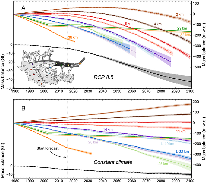
Figure 9. Cumulative daily mass balances using (A) the RCP 8.5 scenario and (B) the constant climate scenario. For both scenarios, glacier-wide balances over the entire glacier (in Gt, left axis) and point balances at the index sites (in m w.e., right axis) are shown. The index sites are annotated with locations given on the inset map in (A). Bold lines indicate the means derived from the 400 Monte Carlo runs; semi-transparent areas delimit the corresponding standard deviations. In the case of the index sites, the curves terminate once 5% of the model runs indicate ice-free conditions (an existing curve thus reflects at least 95% probability for ice at the index sites). Abruptly increasing standard deviations at selected lower-lying stakes (e.g., L-22 km) are due to the fact that the stakes are debris-covered in some model runs, while not in others. Index site 38 km got covered by moraine debris in 2015, so that the stake's mass balance curve flattens with the start of the forecasting period.

FIGURE 10

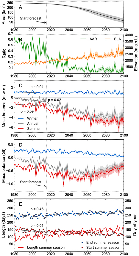
Figure 10. Evolution of (A) glacier area, (B) AAR and ELA and (C–D) annual and seasonal glacier-wide mass balances (stratigraphic time system) during the period 1980–2100, using the RCP 8.5 scenario. (E) Evolution of the summer season length (left axis) and start/end dates of the summer seasons (right axis). In (A–D), bold colored lines indicate the means of the results of all Monte Carlo runs while the semi-transparent areas delimit the corresponding standard deviations. In (E), lines and points indicate the means of the Monte Carlo runs. In (C,E), bold black lines show trend lines fitted over the hindcasting period, with p values indicating the degree of statistical significance.

5.1.1. Index Sites

Of the 12 index site locations, only two (2 and 4 km) are located in the accumulation zone over the entire hindcasting period (Figure 9A). The cumulative mass balance at index site 8 km is slightly positive over the hindcasting period, though only due to the residual mass accumulated in the early hindcasting period. Over the latter part of the hindcasting period the 8 km index site is close to the glacier's equilibrium line, with both positive and negative mass-balance years occurring. Index site 11 km shows a similar pattern: while just at the equilibrium line in the early hindcasting period, it is located in the ablation zone in most of the recent years. The index sites 26–32 km are affected by the 2002 rockslide deposits, which cause subdued annual mass balance cycles after 2002. Toward the end of the hindcasting period, the cumulative mass balances of the index sites 26–32 km approach those of the index sites L-22 km and 20 km, which are located ~200–400 m higher on the glacier. Index site 38 km close to the present terminus has the most negative surface mass balance, accumulating to −229.1 ± 4.8 m w.e. over the mass-balance years 1980–2015.

5.1.2. Mass-Balance Trends

Both the winter and summer balances, and thus the annual balances, show negative trends, implying decreasing mass accumulation in the winter season and increasing mass loss in the summer season (Figure 10C). The trends, fitted by linear regression, are significant at the 0.05 and 0.1 levels, with the summer trend nearly twice as negative as the winter trend. The negative trends coincide with summer seasons becoming longer (Figure 10E). The extension of the summer season occurs in spring only: while the summer season sets in earlier over time (significant at the 0.01 level), no significant trend is observed with regard to its end date (p = 0.46). The 1979–2015 climate data indicates warming in the summer and precipitation decrease in the winter (both significant at the 0.05 level) as the main drivers for the negative mass balance trends. Summer precipitation and winter temperature show no significant trends.

5.1.3. Feedbacks

The hindcasting period is characterized by increasing debris cover and glacier retreat, both of which exert negative feedbacks on the glacier-wide specific mass balances. Yet the model indicates increasingly negative mass balances, so that the atmospheric warming and the positive climate-elevation feedback must exceed the combined effects of the negative feedbacks. To evaluate the relative strengths of the climate-elevation feedback and the feedback due to glacier retreat, we ran the mass balance model without adapting the glacier's geometry (i.e., on the 1980 reference-surface, Elsberg et al., 2001) and compared the resulting specific mass balances to our conventional hindcasting runs. The conventional balances are more negative, though only slightly, indicating that the positive climate-elevation feedback is stronger than the negative feedback due to glacier retreat (Figure S7). This suggests the glacier's adaptation leads to a geometry more susceptible to warming than without adaptation, setting the stage for unstable thinning similar to other glaciers in Alaska (e.g., Trüssel et al., 2015).

5.1.4. Effect of Rockslide Deposits

Black Rapids' negative mass balance trend would be amplified without deposition of the 2002 rockslide debris. While the rockslide deposits are ~4.5 m thick on average (Kienholz et al., 2016), the deposits' surfaces were located ~15 m above the surrounding ice surface in 2007, only 5 years after the rockslides occurred (Shugar and Clague, 2011). To evaluate the rockslides' effect on the glacier-wide mass balance quantitatively, we compared the conventional hindcasting runs to runs without debris layer updates after 2002. Between the 2003 and 2015 mass-balance years, the glacier-wide cumulative mass balances differ by ~20% (Figure S8) although the rockslide deposits make up only ~4.5% of the total glacier area. The deposits' strong impact is due to their location in the lower ablation zone (between ~1,000 and 1,400 m a.s.l., Figure 1), where their melt suppression applies over a longer period than at higher, colder elevations.

5.1.5. Comparison to Gulkana Glacier

Gulkana Glacier is a USGS benchmark glacier located ~40 km to the southeast of Black Rapids. USGS benchmark glaciers were chosen initially to represent entire glacierized regions (e.g., Mayo and Trabant, 1986; Echelmeyer et al., 1996), which prompts a comparison between our modeled Black Rapids mass balances and those measured at Gulkana. Gulkana's conventional mass balances are derived by integrating in situ observations across a regularly updated glacier hypsometry (van Beusekom et al., 2010; O'Neel et al., 2014). Relying on short-duration mass balance modeling (van Beusekom et al., 2010), the USGS obtains glacier-wide balances in the stratigraphic time system (i.e., with annual mass balances reaching from one annual glacier-wide mass minimum to the next), which we compare to the Black Rapids balances in the same time system. On average, Black Rapids' annual mass balances are slightly more positive than those of Gulkana Glacier (by 0.09 m w.e. a⁻¹, Figure 11). Evaluation of the seasonal balances shows that Black Rapids' summer balances are less negative than those of Gulkana Glacier (by 0.3 m w.e.) while the winter balances are less positive (by 0.2 m w.e.). These seasonal differences may be related to greater debris coverage at Black Rapids Glacier and higher winter precipitation at Gulkana Glacier (Kienholz et al., 2016), however, such interpretations are complicated by the glacier's different hypsometries. The annual balances of the two glaciers each describe 75% of the other's balance variability (r² = 0.75, Figure 11B), which is notable given the different properties (size, geometry, debris cover) of the two glaciers (Kienholz et al., 2016). As expected, the summer balances of the two glaciers correlate much better (r² = 0.81) than the winter balances (r² = 0.36), the latter of which are more dependent on local conditions (e.g., topography, McGrath et al., 2015). Comparison of the summer season lengths (Figure 11C) indicates a very good match after 1995, but more variability before that, mostly due to differences in the start of the summer seasons. Overall, this analysis reinforces Gulkana's representative status for other glaciers in the region, though additional comparisons with other glaciers remain desired.

FIGURE 11

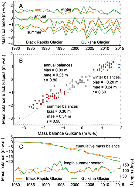
Figure 11. (A) Glacier-wide specific mass balances for Black Rapids Glacier (orange, this study) and Gulkana Glacier (green, O'Neel et al., 2014) during the period 1980–2015. Both series reflect conventional balances (i.e., obtained with regularly updated glacier hypsometries/extents) in the stratigraphic time system (i.e., with annual mass balances reaching from one annual glacier-wide mass minimum to the next and winter (summer) balances reaching from the annual glacier-wide minimum (maximum) to the maximum (minimum)). (B) Specific mass balances of Gulkana Glacier vs. Black Rapids Glacier, with corresponding statistical parameters. (C) Cumulative series of the annual glacier-wide mass balances (left axis) and evolution of the summer season length (right axis).

5.1.6. Uncertainties

The range in our modeled results, arising from the choice of the parameters during the Monte Carlo runs, is relatively small. Over the mass-balance years 1980–2015, the most positive and negative glacier-wide cumulative mass balances differ by only ~0.2 Gt from the mean, which corresponds to ± 5% of the total change modeled (4.0 Gt). While the modeled mass balance is affected primarily by the choice of the mass balance model parameter combinations, the modeled glacier area is also affected by the choice of the density values during the Monte Carlo runs. Here, the smallest and largest area changes differ by ~20% from the mean.

5.2. Projections

5.2.1. GFDL-CM3 RCP 8.5 Scenario

Our projections for the RCP 8.5 scenario indicate very negative surface mass balances throughout the Twenty-first century (Figure 9A). Over the mass-balance years 2016–2100 Black Rapids Glacier will lose 38.1 ± 6.2 Gt of ice (Figure 10A). The mass loss will be accompanied by glacier retreat (174.2 ± 19.7 km² over the mass-balance years 2016–2100), with 67.3 ± 20.3 km² (~28% of its 2010 area) of glacier area remaining by the end of the Twenty-first century. Figure 12A illustrates the modeled ice extents for the years 2025, 2050, 2075, and 2100 using probabilities based on extents from the 400 Monte Carlo runs. Figure S9A shows the corresponding probabilities for debris-cover extent.

FIGURE 12

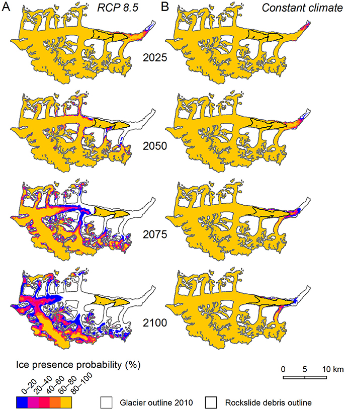
Figure 12. Probability of the presence of ice for the years 2025, 2050, 2075, and 2100 for (A) the RCP 8.5 and (B) the constant climate scenarios. The probabilities are calculated from the stacked extents, where one extent reflects one Monte Carlo run. The locations of the rockslide debris are shown with black outlines. Note that this figure shows areal changes. Thinning may occur even if the ice presence probability is 100%.

By the middle of the century, all index sites will be in the ablation zone (Figure 9A). The mass balances at the index sites will become increasingly negative, with trends altered locally by the evolving debris cover. Moraine debris-covered index site 38 km became debris-covered in 2015 (according to the last Landsat-derived debris grid), suppressing the site's negative mass balance trend while also increasing the uncertainties (due to the large range of d values in our final parameter solutions). The step change in the mass balance trend of site 26 km in 2025 reflects the down-glacier advection of the rockslide debris, which is modeled to give way to moraine debris that year.

Over the course of the projection period, the ELAs rise from the current ~1,900 m a.s.l. to ~2,800 m a.s.l. and the AARs reach consistently low values around 0.1 (Figure 10B). The specific mass balances become increasingly negative, reaching −4 m w.e. in 2080 (Figure 10C). This suggests the glacier will evolve into a state of increasing imbalance with the projected climate. Remarkably, this occurs despite the strong glacier retreat (Figure 10A), which exerts a negative feedback on the specific mass balances. Only after 2080 is glacier recession sufficient to counteract a further decrease of the specific mass balances. By then, the glacier will have lost most of its valley portion and lie in steeper terrain (Figure 12A), which strengthens the negative feedback from retreat. To ultimately stabilize the glacier, a trend toward a balanced mass budget is required, however, such a trend is not projected by the model. Given the small glacier area above 2100's projected ELA (~2,800 m a.s.l.), Black Rapids Glacier will likely vanish almost completely within the first decades of the Twenty-second century.

Throughout the projection period, the winter seasons become significantly shorter (decreasing from ~250 to 200 days) due to both earlier onset and delayed termination of the summer season (which increases in length from ~100 to 150 days, Figure 10E). Yet the specific winter balances remain constant over the entire period (Figure 10C), likely due to the projected precipitation increase and the glacier's retreat to higher elevations, where precipitation is increased due to orographic effects. The negative progression of the annual balances is thus caused solely by the summer balances, which become very negative due to both higher temperatures and longer summer seasons.

The behavior of the glacier-wide mass loss (in Gt), which is closely related to the glacier runoff, deviates from the glacier-wide specific mass balance (in m w.e.). The mass loss increases initially, but flattens out at around 2040 and starts to decrease after around 2060 (Figure 10D). By that time, the glacier will have shrunk sufficiently that the glacier-wide mass loss will decrease despite record-negative specific mass balances. This implies Black Rapids' annual runoff will reach its maximum around the period 2050–2070 and then decrease sharply. In 2100, the runoff may have similar magnitude to that of today, however, it may differ in timing and also enter the watershed much higher in elevation than currently.

5.2.2. Constant Climate Scenario

The constant climate scenario, repeating the climate of the period 1985–2010, indicates negative mass balances and glacier retreat, however, with changes much less distinct than modeled for the RCP 8.5 scenario. The model projects 12.6 ± 1.9 km² of glacier retreat over the mass-balance years 2016–2100, with 228.8 ± 2.8 km² of glacier area (~95% of its 2010 area) remaining in 2100 (Figure 12B, Figure S9B). The corresponding mass loss is 5.7 ± 1.0 Gt over the mass-balance years 2016–2100 (Figure 9B, Figure S10).

The glacier-wide annual mass loss is decreasing over the course of the projection period (Figure S10D), primarily reflecting the decrease in glacier area. The annual specific mass balance is decreasing also (Figure S10C), albeit only slightly, suggesting that the positive feedback due to glacier thinning (climate-elevation feedback) competes effectively with the negative feedback due to glacier retreat. Black Rapids Glacier remains in a state of imbalance throughout the projection period, suggesting continued retreat after 2100. According to our model experiments, the unstable thinning detected during the hindcasting period (conventional balances < reference balances) is not maintained during the entire forecasting period, with the cumulative conventional balances exceeding the reference balances at ~2038 (Figure S7).

The fact that Black Rapids Glacier is unlikely to achieve a balanced state in the Twenty-first century, even under constant climate, raises the question how much of its valley portion Black Rapids could sustain longer term if the current climate prevailed. To assess this question, we ran the glacier model until 2700, repeating the constant climate every 35 years. The results from this experiment suggest considerable retreat, with only ~170 km² of glacier area remaining in 2700 (Figure S11). Black Rapids is projected to gradually approach steady state toward the end of the modeling period, with 35 year averages of the specific mass balances close to zero and AARs around 0.6. Despite the large uncertainties (e.g., uncertain debris-cover evolution, no advance allowed in the retreat parametrization), this experiment highlights Black Rapids' distinct sensitivity to climate change and demonstrates the long time scales over which the glacier adjusts its shape. Both high sensitivity to climate change and long adjustment time scales are a result of Black Rapids' thick, low-slope valley portion.

5.3. Implications for Surge Likelihood

While the mechanisms for surge initiation are not fully understood (e.g., Harrison and Post, 2003), it is commonly accepted that the surge reservoir needs to reach a certain critical geometry for a next surge to occur. Slope and ice thickness both control the glacier's basal shear stress, which may ultimately trigger a surge upon reaching critical level. Black Rapids' critical geometry is unknown due to the lack of observations prior to the 1936–1937 surge. For the same reason, precise delineation of Black Rapids' surge reservoir is difficult, though the reservoir most likely encompasses the entire area above index site 20 km (i.e., above the Loket confluence, Heinrichs et al., 1995). Our analysis focuses on the surge reservoir of Black Rapids' main branch, given the availability of in situ elevation and mass balance measurements, and the fact that surge initiation most likely occurs in this area.

With the glacier geometry considered a key factor for surge initiation, our surge likelihood assessment focuses on the reservoir's response to the negative mass balance trend. In the case of Black Rapids, surface elevation changes were measured at individual index sites over parts of the hindcasting period (Heinrichs et al., 1995; Truffer et al., 2005). Combined with surface mass balance measurements (and assuming negligible elevation changes due to firn-related processes), they allow for the derivation of time-averaged ice flow emergence velocities, which in turn allow converting the modeled mass balance time series into continuous surface elevation time series. We calculated such elevation time series for the index sites 4, 8, 14, and 20 km, all of which are located in the surge reservoir. The emergence velocities at these four sites, −0.75, −0.10, 1.00, and 2.25 m w.e. a⁻¹, were derived from surface elevation changes between 1980 and 2010 (Kienholz et al., 2016) and the corresponding cumulative surface mass balances. To hypothesize about the surface elevation changes in the near future, we continued the time series until 2035, based on the modeled surface mass balances from the RCP 8.5 scenario. We refrained from projections beyond 2035 as the assumption of constant emergence velocities becomes increasingly unrealistic (changing glacier geometry may affect ice flow considerably). Even for the hindcasting period, the assumption of constant emergence velocities is uncertain in light of Black Rapids' complex flow behavior (Heinrichs et al., 1996). As a consequence, the temporal variations in the derived surface elevations need to be interpreted cautiously.

Figure 13 shows the mass balance, emergence velocity and elevation change time series until 2035. From the start of the modeling period until ~1988, the computed cumulative elevation changes indicate ice thickening at all four sites. This period corresponds to the period with relatively favorable glacier-wide mass balances (Section 5.1). Interestingly, neighboring West Fork Glacier surged in 1987–1988 (Harrison et al., 1994), just at the end of this period. The negative trend after 1988 includes all four sites, however, it is particularly pronounced for the two lower-lying sites 14 and 20 km. While they are calculated to lose ~9 and 15 m over the entire hindcasting period, the net elevation change at the sites 4 and 8 km is close to zero. Over the forecasting period, the projected elevation loss becomes increasingly pronounced due to the very negative mass balances under the RCP 8.5 scenario. Assuming constant emergence velocities, the index sites' locations are projected to lose between ~30 (site 4 km) and 60 m (site 20 km) of ice until 2035.

FIGURE 13

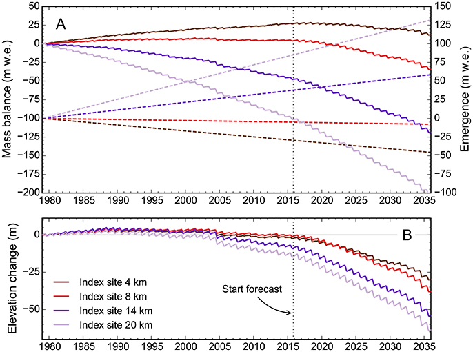
Figure 13. (A) Cumulative daily surface mass balance (solid lines, left axis) and ice flow emergence (dashed lines, right axis) for four selected index sites in the surge reservoir, over the time period 1979–2035. (B) Cumulative elevation change, corresponding to the difference between surface mass balance and flow emergence. The vertical scale in (B) is twice as large as in (A).

Overall, these results indicate a surge is unlikely to occur in the near future due to mass starvation and corresponding lack of thickening in the reservoir area. This conclusion, which supports conjectures from previous studies (Kienholz et al., 2016), applies to the current climate and to the projected climate under the RCP 8.5 scenario. To re-initiate thickening in the surge reservoir, the surface mass balances would need to be at least as favorable as they were in the early 1980s.

6. Conclusion

We employed a surface mass balance model coupled to retreat and debris models to assess the evolution of surge-type Black Rapids Glacier throughout the Twenty-first century. The modeling indicates Black Rapids Glacier is greatly out of balance with the current and projected climate. The glacier model shows approximate equilibrium only for the early hindcasting period (1980–1988). A negative mass balance trend emerges thereafter, caused by atmospheric warming in the summer, precipitation decrease in the winter and surface elevation lowering (climate-elevation feedback), which exceed the moderating effects from increasing debris cover and glacier retreat. Without the 2002 rockslide deposits, the mass balance trend would be considerably more negative, by ~20% between the 2003 and 2015 mass-balance years. The negative mass-balance trend is predicted to continue through the forecasting period. With the constant climate scenario, Black Rapids is projected to lose ~8% of its 1980 area by 2100, of which 3% had been lost at the beginning of the forecasting period already. By 2100, Black Rapids Glacier will not have achieved a state of equilibrium with the climate, even under constant climate. Thus, additional thinning and retreat will occur after 2100, ultimately causing the loss of large parts of Black Rapids' valley portion. With the GFDL-CM3 RCP 8.5 scenario, the modeled glacier wastage is yet accelerated, with ~73% area loss relative to 1980. The small glacier portions remaining will be in a pronounced state of imbalance with the climate and vanish in the first decades of the Twenty-second century, except for a few ice remnants above 2100's projected ELA (lying at ~2,800 m a.s.l.).

In this study, we have used the reanalysis by Bieniek et al. (2016) and the corresponding downscaled RCP 8.5 scenario by Lader et al. (submitted) for the first time for a glaciological application. The quality of these Alaska-wide climate products marks a step forward compared to climate data used in previous glacier studies (e.g., Ziemen et al., 2016). Improved quality of this key input variable, and the fact that for the first time we used a large range of Black Rapids-specific measurements for the mass balance model calibration, improved the accuracy of our results. Considering debris evolution, which is not yet standard in glaciological studies, further increased the quality of our projections. Finally, we quantified the remaining uncertainties systematically with a Monte Carlo approach, which improved on the widely used approach of choosing one single optimal input/parameter combination (which lacks this uncertainty information).

Despite these advancements, several improvements could help further reduce the uncertainties in our results. An ice thickness map derived from local data (mass balances, thickness measurements) would likely improve on the global product used here. Ideally, such a new ice thickness map would come with an uncertainty mask. This would allow for propagating the thickness uncertainties into our model results in a more sophisticated way than is done currently. Sophisticated approaches for ice thickness derivation exist (e.g., Brinkerhoff et al., 2016), however, their application benefits substantially from high quality ice velocity fields, which we do not possess currently for Black Rapids Glacier. WRF-downscaled climate data with higher spatial resolution would be ideal to mitigate potential problems arising from our simple statistical downscaling, which, for example, fails to conserve mass and energy. In the absence thereof, the additional downscaling from 20 km to 100 m may be improved by applying an approach based on the linear theory of orographic precipitation (Smith and Barstad, 2004). Application of an actual ice flow model may further improve our results, for example, by reproducing thinning rates that vary among Black Rapids' branches (Kienholz et al., 2016), which cannot be achieved with our retreat parametrization. Besides modeling a more realistic glacier evolution, a flow model would yield ice flow velocities useful for sophisticated projections of future debris cover (e.g., Rowan et al., 2015). A debris thickness map would allow for more sophisticated melt modeling in debris-covered areas (e.g., Reid et al., 2012; Carenzo et al., 2016). Such a debris thickness map could be obtained by combining new remotely sensed techniques (e.g., Schauwecker et al., 2015) and in situ debris thickness measurements. Despite room for improvement on the glacier model side, the greatest source of uncertainty is the evolution of the future climate, as shown in this study by modeling with lower and a higher bound scenarios. Constraining this evolution will thus be critical for more accurate glacier predictions.

Author Contributions

CK developed methods, implemented the code and wrote the paper. RH provided guidance and feedback throughout the project and helped to write the paper. MT collected field data, partly with the help of CK, and provided comments on the methods and the paper. PB and RL contributed climate data and commented on the paper.

Conflict of Interest Statement

The authors declare that the research was conducted in the absence of any commercial or financial relationships that could be construed as a potential conflict of interest.

Acknowledgments

We thank B. Anderson for sharing and discussing his glacier model code during CK's research stay at the Victoria University of Wellington (funded by the S. T. Lee Young Researcher Award), which inspired the development of this glacier model. We further thank A. Roth for help with the model code development and R. Wastlhuber for processing one of the snow line elevation datasets. S. O'Neel is acknowledged for providing the Gulkana Glacier mass balances, M. Huss for the Black Rapids ice thicknesses, and A. Arendt for computational resources and funding. K. Echelmeyer, M. Stuefer, and R. Flanders were instrumental in maintaining the mass balance program on Black Rapids Glacier during the 1990s and 2000s. C. Larsen has contributed to the mass balance program over the recent years. This work was funded by grants from NSF (OPP-1107491), NASA (NNX11AF41G) and the U.S. Department of the Interior Climate Science Center. CK was also funded by a fellowship from the UAF graduate school. PB and RL acknowledge funding from the U.S. Geological Survey (grant G10AC00588).

Supplementary Material

The Supplementary Material for this article can be found online at: https://www.frontiersin.org/article/10.3389/feart.2017.00056/full#supplementary-material

References

Arendt, A., Walsh, J., and Harrison, W. (2009). Changes of glaciers and climate in northwestern North America during the late twentieth century. J. Climatol. 22, 4117–4134. doi: 10.1175/2009JCLI2784.1

CrossRef Full Text | Google Scholar

Bevington, A., and Copland, L. (2014). Characteristics of the last five surges of Lowell Glacier, Yukon, Canada, since 1948. J. Glaciol. 60, 113–123. doi: 10.3189/2014JoG13J134

CrossRef Full Text | Google Scholar

Bieniek, P. A., Bhatt, U. S., Thoman, R. L., Angeloff, H., Partain, J., Papineau, J., et al. (2012). Climate divisions for Alaska based on objective methods. J. Appl. Meteorol. Climatol. 51, 1276–1289. doi: 10.1175/JAMC-D-11-0168.1

CrossRef Full Text | Google Scholar

Bieniek, P. A., Bhatt, U. S., Walsh, J. E., Rupp, T. S., Zhang, J., Krieger, J. R., et al. (2016). Dynamical downscaling of ERA-Interim temperature and precipitation for Alaska. J. Appl. Meteorol. Climatol. 55, 635–654. doi: 10.1175/JAMC-D-15-0153.1

CrossRef Full Text | Google Scholar

Bieniek, P. A., Walsh, J. E., Thoman, R. L., and Bhatt, U. S. (2014). Using climate divisions to analyze variations and trends in Alaska temperature and precipitation. J. Clim. 27, 2800–2818. doi: 10.1175/JCLI-D-13-00342.1

CrossRef Full Text | Google Scholar

Brinkerhoff, D. J., Aschwanden, A., and Truffer, M. (2016). Bayesian inference of subglacial topography using mass conservation. Front. Earth Sci. 4:8. doi: 10.3389/feart.2016.00008

CrossRef Full Text | Google Scholar

Brooks, P. D. (1988). The Alaska High-Altitude Aerial Photography (AHAP) Program. Technical report, State of Alaska.

Cannon, A. J., Sobie, S. R., and Murdock, T. Q. (2015). Bias correction of GCM precipitation by quantile mapping: how well do methods preserve changes in quantiles and extremes? J. Climate 28, 6938–6959. doi: 10.1175/JCLI-D-14-00754.1

CrossRef Full Text | Google Scholar

Carenzo, M., Pellicciotti, F., Mabillard, J., Reid, T., and Brock, B. (2016). An enhanced temperature index model for debris-covered glaciers accounting for thickness effect. Adv. Water Resour. 94, 457–469. doi: 10.1016/j.advwatres.2016.05.001

PubMed Abstract | CrossRef Full Text | Google Scholar

Cogley, J. G., Hock, R., Rasmussen, L. A., Arendt, A. A., Bauder, A., Braithwaite, R. J., et al. (2011). Glossary of Glacier Mass Balance and Related Terms. IHP-VII Technical Documents in Hydrology, 86.

Daly, C., Neilson, R. P., and Phillips, D. L. (1994). A statistical-topographic model for mapping climatological precipitation over mountainous terrain. J. Appl. Meteorol. 33, 140–158. doi: 10.1175/1520-0450(1994)033<0140:ASTMFM>2.0.CO;2

CrossRef Full Text | Google Scholar

Dee, D., Uppala, S., Simmons, A., Berrisford, P., Poli, P., Kobayashi, S., et al. (2011). The ERA-interim reanalysis: configuration and performance of the data assimilation system. Q. J. R. Meteorol. Soc. 137, 553–597. doi: 10.1002/qj.828

CrossRef Full Text | Google Scholar

Donner, L. J., Wyman, B. L., Hemler, R. S., Horowitz, L. W., Ming, Y., Zhao, M., et al. (2011). The dynamical core, physical parameterizations, and basic simulation characteristics of the atmospheric component AM3 of the GFDL global coupled model CM3. J. Climate 24, 3484–3519. doi: 10.1175/2011JCLI3955.1

CrossRef Full Text | Google Scholar

Echelmeyer, K., Harrison, W., Larsen, C., Sapiano, J., Mitchell, J., DeMallie, J., et al. (1996). Airborne surface profiling of glaciers: a case-study in Alaska. J. Glaciol. 42, 538–547. doi: 10.1017/S002214300000352X

CrossRef Full Text | Google Scholar

Eisen, O., Harrison, W., and Raymond, C. (2001). The surges of Variegated Glacier, Alaska, USA, and their connection to climate and mass balance. J. Glaciol. 47, 351–358. doi: 10.3189/172756501781832179

CrossRef Full Text | Google Scholar

Elsberg, D. H., Harrison, W. D., Echelmeyer, K. A., and Krimmel, R. M. (2001). Quantifying the effects of climate and surface change on glacier mass balance. J. Glaciol. 47, 649–658. doi: 10.3189/172756501781831783

CrossRef Full Text | Google Scholar

Flowers, G., Roux, N., Pimentel, S., and Schoof, C. (2011). Present dynamics and future prognosis of a slowly surging glacier. Cryosphere 5, 299–313. doi: 10.5194/tc-5-299-2011

CrossRef Full Text | Google Scholar

Gades, A. M. (1998). Spatial and Temporal Variations of Basal Conditions Beneath Glaciers and Ice Sheets Inferred from Radio Echo Soundings. Ph.D. thesis, University of Washington.

Harrison, W., Echelmeyer, K., Chacho, E., Raymond, C., and Benedict, R. (1994). The 1987–88 surge of West Fork Glacier, Susitna Basin, Alaska, USA. J. Glaciol. 40, 241–254. doi: 10.1017/S0022143000007334

CrossRef Full Text | Google Scholar

Harrison, W. D., and Post, A. S. (2003). How much do we really know about glacier surging? Ann. Glaciol. 36, 1–6. doi: 10.3189/172756403781816185

CrossRef Full Text | Google Scholar

Heinrichs, T., Mayo, L., Trabant, D., and March, R. (1995). Observations of the Surge-Type Black Rapids Glacier, Alaska, during a Quiescent Period, 1970–92. Open-file report 94–512, U.S. Geological Survey.

Google Scholar

Heinrichs, T. A., Mayo, L., Echelmeyer, K., and Harrison, W. (1996). Quiescent-phase evolution of a surge-type glacier: Black Rapids Glacier, Alaska, USA. J. Glaciol. 42, 110–122. doi: 10.3189/172756403781816185

CrossRef Full Text | Google Scholar

Hock, R. (1999). A distributed temperature-index ice- and snowmelt model including potential direct solar radiation. J. Glaciol. 45, 101–111. doi: 10.1017/S0022143000003087

CrossRef Full Text | Google Scholar

Hulth, J., Rolstad Denby, C., and Hock, R. (2013). Estimating glacier snow accumulation from backward calculation of melt and snowline tracking. Ann. Glaciol. 54, 1–7. doi: 10.3189/172756413807342965

CrossRef Full Text | Google Scholar

Huss, M., and Farinotti, D. (2012). Distributed ice thickness and volume of all glaciers around the globe. J. Geophys. Res. 117:F04010. doi: 10.1029/2012JF002523

CrossRef Full Text | Google Scholar

Huss, M., Jouvet, G., Farinotti, D., and Bauder, A. (2010). Future high-mountain hydrology: a new parameterization of glacier retreat. Hydrol. Earth Syst. Sci. 14, 815–829. doi: 10.5194/hess-14-815-2010

CrossRef Full Text | Google Scholar

Kienholz, C., Herreid, S., Rich, J., Arendt, A., Hock, R., and Burgess, E. (2015). Derivation and analysis of a complete modern-date glacier inventory for Alaska and northwest Canada. J. Glaciol. 61, 403–420. doi: 10.3189/2015JoG14J230

CrossRef Full Text | Google Scholar

Kienholz, C., Hock, R., Truffer, M., Arendt, A. A., and Arko, S. (2016). Geodetic mass balance of surge-type Black Rapids Glacier, Alaska, 1980–2001–2010, including role of rockslide deposition and earthquake displacement. J. Geophys. Res. Earth Surf. 121, 1–24. doi: 10.1002/2016JF003883

CrossRef Full Text | Google Scholar

Lang, H. (1968). “Relations between glacier runoff and meteorological factors observed on and outside the glacier,” in IUGG General Assembly, Vol. 79, (Bern: International Association of Scientific Hydrology), 429–439.

Larsen, C., Burgess, E., Arendt, A., O'Neel, S., Johnson, A., and Kienholz, C. (2015). Surface melt dominates Alaska glacier mass balance. Geophys. Res. Lett. 42, 5902–5908. doi: 10.1002/2015GL064349

CrossRef Full Text | Google Scholar

Machguth, H., Paul, F., Kotlarski, S., and Hoelzle, M. (2009). Calculating distributed glacier mass balance for the Swiss Alps from regional climate model output: a methodical description and interpretation of the results. J. Geophys. Res. 114:D19106. doi: 10.1029/2009JD011775

CrossRef Full Text | Google Scholar

Mayo, L., and Trabant, D. (1986). Recent growth of Gulkana Glacier, Alaska Range, and its relation to glacier-fed river runoff. U.S. Geol. Survey Bull. 2290, 91–99.

Google Scholar

McGrath, D., Sass, L., O'Neel, S., Arendt, A., Wolken, G., Gusmeroli, A., et al. (2015). End-of-winter snow depth variability on glaciers in Alaska. J. Geophys. Res. Earth Surf. 120, 1530–1550. doi: 10.1002/2015JF003539

CrossRef Full Text | Google Scholar

O'Neel, S., Hood, E., Arendt, A., and Sass, L. (2014). Assessing streamflow sensitivity to variations in glacier mass balance. Climatic Change 123, 329–341. doi: 10.1007/s10584-013-1042-7

CrossRef Full Text | Google Scholar

Pfeffer, W. T., Arendt, A. A., Bliss, A., Bolch, T., Cogley, J. G., Gardner, A. S., et al. (2014). The Randolph Glacier Inventory: a globally complete inventory of glaciers. J. Glaciol. 60, 537–552. doi: 10.3189/2014JoG13J176

CrossRef Full Text | Google Scholar

Radić, V., Bliss, A., Beedlow, A. C., Hock, R., Miles, E., and Cogley, J. G. (2014). Regional and global projections of twenty-first century glacier mass changes in response to climate scenarios from global climate models. Climate Dyn. 42, 37–58. doi: 10.1007/s00382-013-1719-7

CrossRef Full Text | Google Scholar

Reid, T. D., Carenzo, M., Pellicciotti, F., and Brock, B. W. (2012). Including debris cover effects in a distributed model of glacier ablation. J. Geophys. Res. Atmospheres 117:D18105. doi: 10.1029/2012JD017795

CrossRef Full Text | Google Scholar

Riahi, K., Rao, S., Krey, V., Cho, C., Chirkov, V., Fischer, G., et al. (2011). RCP 8.5–A scenario of comparatively high greenhouse gas emissions. Climatic Change 109, 33–57. doi: 10.1007/s10584-011-0149-y

CrossRef Full Text | Google Scholar

Rowan, A. V., Egholm, D. L., Quincey, D. J., and Glasser, N. F. (2015). Modelling the feedbacks between mass balance, ice flow and debris transport to predict the response to climate change of debris-covered glaciers in the Himalaya. Earth Planet. Sci. Lett. 430, 427–438. doi: 10.1016/j.epsl.2015.09.004

CrossRef Full Text | Google Scholar

Sanford, T., Frumhoff, P. C., Luers, A., and Gulledge, J. (2014). The climate policy narrative for a dangerously warming world. Nat. Clim. Change 4, 164–166. doi: 10.1038/nclimate2148

CrossRef Full Text | Google Scholar

Schaefer, M., Machguth, H., Falvey, M., and Casassa, G. (2013). Modeling past and future surface mass balance of the Northern Patagonia Icefield. J. Geophys. Res. Earth Surf. 118, 571–588. doi: 10.1002/jgrf.20038

CrossRef Full Text | Google Scholar

Schauwecker, S., Rohrer, M., Huggel, C., Kulkarni, A., Ramanathan, A., Salzmann, N., et al. (2015). Remotely sensed debris thickness mapping of Bara Shigri Glacier, Indian Himalaya. J. Glaciol. 61, 675–688. doi: 10.3189/2015JoG14J102

CrossRef Full Text | Google Scholar

Sevestre, H., and Benn, D. I. (2015). Climatic and geometric controls on the global distribution of surge-type glaciers: implications for a unifying model of surging. J. Glaciol. 61, 646–662. doi: 10.3189/2015JoG14J136

CrossRef Full Text | Google Scholar

Shugar, D. H., and Clague, J. J. (2011). The sedimentology and geomorphology of rock avalanche deposits on glaciers. Sedimentology 58, 1762–1783. doi: 10.1111/j.1365-3091.2011.01238.x

CrossRef Full Text | Google Scholar

Shugar, D. H., Rabus, B. T., and Clague, J. J. (2010). Elevation changes (1949–1995) of Black Rapids Glacier, Alaska, derived from a multi-baseline InSAR DEM and historical maps. J. Glaciol. 56, 625–634. doi: 10.3189/002214310793146278

CrossRef Full Text | Google Scholar

Shugar, D. H., Rabus, B. T., Clague, J. J., and Capps, D. M. (2012). The response of Black Rapids Glacier, Alaska, to the Denali earthquake rock avalanches. J. Geophys. Res. Earth Surf. 117:F01006. doi: 10.1029/2011JF002011

CrossRef Full Text | Google Scholar

Skamarock, W. C., Klemp, J. B., Dudhia, J., Gill, D. O., Barker, D. M., Huang, X., et al. (2008). A Description of the Advanced Research WRF Version 3. Technical report, NCAR Technical Notes, Boulder, CO.

Google Scholar

Smith, R. B., and Barstad, I. (2004). A linear theory of orographic precipitation. J. Atmospher. Sci. 61, 1377–1391. doi: 10.1175/1520-0469(2004)061<1377:ALTOOP>2.0.CO;2

CrossRef Full Text | Google Scholar

Sold, L., Huss, M., Hoelzle, M., Andereggen, H., Joerg, P. C., and Zemp, M. (2013). Methodological approaches to infer end-of-winter snow distribution on alpine glaciers. J. Glaciol. 59, 1047–1059. doi: 10.3189/2013JoG13J015

CrossRef Full Text | Google Scholar

Truffer, M., Harrison, W. D., and March, R. S. (2005). Record negative glacier balances and low velocities during the 2004 heatwave in Alaska, USA: implications for the interpretation of observations by Zwally and others in Greenland. J. Glaciol. 51, 663–664. doi: 10.3189/172756505781829016

CrossRef Full Text | Google Scholar

Trüssel, B. L., Truffer, M., Hock, R., Motyka, R. J., Huss, M., and Zhang, J. (2015). Runaway thinning of the low-elevation Yakutat Glacier, Alaska, and its sensitivity to climate change. J. Glaciol. 61, 65–75. doi: 10.3189/2015JoG14J125

CrossRef Full Text | Google Scholar

van Beusekom, A., O'Neel, S., March, R., Sass, L., and Cox, L. (2010). Reanalysis of Alaskan Benchmark Glacier Mass-Balance Data using the Index Method, Scientific Investigations Report 2010–5247. US Geological Survey.

Google Scholar

Ziemen, F., Hock, R., Aschwanden, A., Khroulev, C., Kienholz, C., Melkonian, A., et al. (2016). Modeling the evolution of the Juneau Icefield between 1971 and 2100 using the Parallel Ice Sheet Model (PISM). J. Glaciol. 62, 199–214. doi: 10.1017/jog.2016.13

CrossRef Full Text | Google Scholar