Evaluation of a Buoyancy and Shear Based Mixing Length for a Turbulence Scheme

1. Introduction

Stable boundary layer (SBL) modeling in numerical weather prediction (NWP) models plays a major role in terms of the predictability of the minimal temperature, surface frost, dew, fog, and low-level jet (LLJ). The prediction of these features is required in sectors such as air quality (Weil, 2012), air and road traffic, agriculture, and wind farming (Hansen et al., 2012). It is still a challenge for global and regional models to represent correctly the SBL (Mahrt, 1998; Viterbo et al., 1999; Beljaars et al., 2012; Holtslag et al., 2013). Turbulent mixing is one of the main processes driving the atmospheric SBL along with surface coupling and radiation. The SBL can be classified into two idealized categories (Mahrt, 1998; Zilitinkevich et al., 2008; Mahrt, 2014). The traditional SBL associated with relatively strong and continuous turbulent mixing and a well-defined boundary-layer height is referred as the weakly stable boundary layer (WSBL). In the very stable regime (VSBL), the turbulence is relatively weak and globally intermittent associated with weak winds. Although this division is not completed and oversimplified (Mahrt, 1998), a unique classification is not yet formulated (e.g., Van de Wiel et al., 2003; Banta, 2008; Mahrt, 2014).

Large-eddy simulation (LES) is a state-of-the-art numerical tool used to study the physical processes and the average effects of turbulence on the development of a boundary layer. LES is frequently used to investigate the SBL (see for example, a WSBL LES review by Beare and Macvean, 2004). A common methodology to develop and improve parameterizations is to compare LES statistics to single column model (SCM; Randall et al., 1996; Hourdin et al., 2013). Over the last decade, such model intercomparisons have been investigated at an international scale within the Global Energy and Water Exchanges (GEWEX) Atmospheric Boundary Layer Study (GABLS, Holtslag, 2006) for WSBLs (Cuxart et al., 2006; Svensson et al., 2011; Bosveld et al., 2014). Previous intercomparison studies have shown that strong variabilities in the mean wind and potential temperature profiles is modeled by SCM. For example, strong diffusivity from first-order turbulence scheme leads to overestimations of the mixing and the surface friction velocity, leading to overestimations of the boundary layer and the LLJ heights (Cuxart et al., 2006) and an underestimation of the turning of the wind (Svensson et al., 2011). Most turbulence parameterizations of NWP models currently use a higher-order scheme (TKE-l) based on a turbulence kinetic energy (TKE) prognostic equation with a diagnostic equation for the mixing length. TKE schemes show better convergence to LES results than first-order schemes. However, the variability between models is still high. A fourth intercomparison (GABLS4) of a VSBL, based on observations from Dome C (East Antarctica), is currently in progress (Bazile et al., 2015).

Differences in TKE-l schemes arise primarily from (i) the mixing length formulation for momentum, heat, and dissipation, (ii) the additional use of stability functions, and (iii) different model constants, which can vary by an order of magnitude. Stability functions may arise from second-order equations (e.g., Mellor and Yamada, 1982) or directly from fits to observational data (e.g., Businger et al., 1971; Dyer, 1974; Duynkerke, 1991). Associated with stability functions, different types of mixing lengths are used in TKE-l schemes with either local or non-local characteristics (Lenderink and Holtslag, 2004). Local formulations can be based on (i) the distance to the boundaries, l = κz (Prandtl, 1925), (ii) the local static stability (Deardorff, 1980), or (iii), more recently, the local vertical wind shear (Hunt, 1988; Tjernström, 1993; Schumann and Gerz, 1995; Grisogono and Enger, 2004; Grisogono and Belušić, 2008; Grisogono, 2010; Venayagamoorthy and Stretch, 2010). Non-local mixing lengths (Bougeault and Lacarrere, 1989; Holtslag and Boville, 1993; Lenderink and Holtslag, 2004) have been introduced for convective conditions when the mixing length depends on the size of the largest eddies and the coherent structures. More examples of mixing length formulations can be found in Cuxart et al. (2006).

The present paper emphasizes the key role of mixing length formulations within a turbulence scheme based on TKE-l closure (Cuxart et al., 2000; Cheng et al., 2002) in the research model Meso-NH (Lafore et al., 1998). Meso-NH can be used in LES or in single-column mode and integrates the same turbulence scheme as the French NWP Application of Research to Operations at Mesoscale model (AROME, Seity et al., 2011). In a stably stratified atmosphere, vertical wind shear is the only positive source of TKE. Therefore, wind shear effects on mixing, which are not currently included, should be taken into account in the length scale formulation. Based on the original buoyancy-based formulation (Bougeault and Lacarrere, 1989), this study proposes a buoyancy-shear combined mixing length. The modified formulation is evaluated by comparing the SCM performance to that of LESs for several stably stratified cases from the literature (Beare et al., 2006; Huang and Bou-Zeid, 2013; Sullivan et al., 2016). A sensitivity study to vertical wind shear and stability is proposed as a first evaluation of the new length formulation with diverse forcing. The modified turbulence scheme is also evaluated against convective cases from the literature (Ayotte et al., 1996; Couvreux et al., 2005) to verify the consistency of the modified model in convective boundary layers.

The paper is organized as follows. Section 2 describes the models used in this study as well as the different simulated cases. Section 3 presents the new mixing length for a TKE-l scheme and the motivations for the proposed formulation. The behavior of the turbulence scheme with the new formulation is further compared to the actual scheme and evaluated against LESs in Section 4 by comparing the mean wind and temperature profiles, the boundary-layer height, and the statistical moments. Concluding remarks are proposed in Section 5.

2. Methods

2.1. The Models

2.1.1. Meso-NH

In this study, we use the non-hydrostatic atmospheric research model Meso-NH (Lafore et al., 1998). This model can be run either in mesoscale, single-column, or three-dimensional explicit large-eddy mode. The specifications of each version are detailed below. The turbulence scheme is based on Redelsperger and Sommeria (1982, 1986) and is presented in detail in Cuxart et al. (2000). Model constants are from Cheng et al. (2002).

The scheme is based on a prognostic equation of the subgrid TKE and a diagnostic mixing length. The dissipation of the subgrid TKE is physically induced by small-scale turbulence. The stronger the smallest eddies are, the more intense the dissipation is. Assuming that the turbulence is stationary and isotropic, dimensional arguments (Kolmogorov, 1941) express ϵ, the dissipation rate of TKE, as

$\begin{array}{ll}ϵ=C_{ϵ}\frac{e^{3/2}}{L_{ϵ}},& (1)\end{array}$

where L_ϵ is the dissipation length, e is the kinetic energy, and C_ϵ = 0.85. Traditionally in TKE-l models, the dissipation closure is realized by assuming that the dissipation length equals the mixing length, i.e., L_ϵ = L_m. The validity of this assumption is discussed in Section 4. Note that a possible solution to avoid this assumption is to estimate the dissipation rate of TKE via an additional prognostic equation (Duynkerke and Driedonks, 1987); this is commonly called the TKE-ϵ model. This solution is beyond the scope of this study.

The shared specifications of the LESs and SCMs are the following. The subgrid length scales are modified near the ground, as suggested by Redelsperger et al. (2001), to match the similarity laws and the values of the free-stream model constants. An absorbing layer is prescribed at the top of the domain to prevent spurious reflections.

2.1.2. The Explicit Model

The specifications of Meso-NH in its explicit mode are detailed in this section. The mixing length L_m is different in the LES and mesoscale modes. In LESs, because the grid cells used are very small compared to the largest eddies and nearly isotropic (see the next section), the mixing length can be linked to the largest subgrid energy-containing eddies, which are the size of the grid cell, $L_m={(\Delta x\Delta y\Delta z)}^{1/3}$ (hereafter DELT). DELT is prescribed in most three-dimensional cases. In a stably stratified atmosphere, most energy-containing eddies are much smaller than those in convective conditions. In several LES cases with strong stratification, the largest subgrid energy-containing eddies are usually smaller than the grid cell size. A second mixing length based on the size of the mesh and reduced by the stratification is then considered, as proposed by Deardorff (1980) (hereafter DEAR), such that

$\begin{array}{ll}{L}_m=min\left({(\Delta x\Delta y\Delta z)}^{1/3},0.76\sqrt{\frac{e}{N^2}}\right),& (2)\end{array}$

where N is the Brunt-Väisälä frequency.

For all LESs presented here, the lateral boundary conditions are periodic. An initial random perturbation of 0.1K is applied to the potential temperature over the entire domain. The grid mesh is horizontally isotropic; the grid lengths in the x- and y-axes are equal. For stably stratified cases, excepting the case indicated in Table 1, the vertical resolution is also equal to the horizontal resolution in the boundary layer (a verification is done a posteriori). However, the vertical grid is stretched in the upper part of the domain to save computing resources. For all the LES simulations, we have checked that the subgrid quantities are negligible (<20%) compared to the total (resolved + subgrid) quantities to ensure that the majority of the turbulent eddies are resolved.

TABLE 1

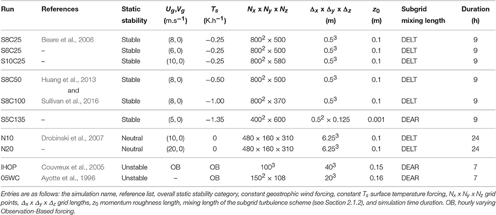
Table 1. Brief description of the LES experiments (see text and references for more details).

2.1.3. The Single-Column Model

The host model Meso-NH can also be used in single-column mode, in which only the vertical mixing is considered. The one-dimensional (1D) turbulence scheme is based on one prognostic equation of the subgrid TKE, e, given by

$\begin{array}{l}\frac{\partial e}{\partial t}={\displaystyle \underset{T}{{\displaystyle \underbrace{-\frac{1}{{\rho }_{ref}}\frac{\partial }{\partial z}\left(C_T{\rho }_{ref}{L}_m\sqrt{e}\frac{\partial e}{\partial z}\right)}}}}{\displaystyle \underset{DP}{{\displaystyle \underbrace{-\overline{u\prime w\prime }\frac{\partial \overline{U}}{\partial z}-\overline{v\prime w\prime }\frac{\partial \overline{V}}{\partial z}}}}}\\ +{\displaystyle \underset{B}{{\displaystyle \underbrace{\frac{g}{{\theta }_{v,ref}}\overline{w\prime \theta \prime }}}}}-{\displaystyle \underset{D}{{\displaystyle \underbrace{C_{ϵ}\frac{e^{3/2}}{L_{ϵ}}}}}},& (3)\end{array}$

where T stands for the Transport term, DP for the Dynamical Production term, D for the Dissipation term and B for the Buoyancy term, which is a production term in a convective stratification and a destructive term in a stable stratification. $\overline{u\prime w\prime }$, $\overline{v\prime w\prime }$, and $\overline{\theta \prime w\prime }$ are the average vertical turbulent momentum and heat fluxes, respectively, and ' denotes the deviation from the mean values. $\overline{U}$, $\overline{V}$, and $\overline{\theta }$, are the horizontal mean velocities and the potential temperature, respectively, and w is the vertical velocity. θ_v,ref and ρ_ref indicate the reference virtual potential temperature and the density from the adiabatic and hydrostatic state. The parameterized turbulent fluxes are expressed as

$\begin{array}{ll}\begin{array}{l}\overline{u\prime w\prime }=-K_m\frac{\partial \overline{U}}{\partial z},\\ \overline{v\prime w\prime }=-K_m\frac{\partial \overline{V}}{\partial z},\\ \overline{\theta \prime w\prime }=-K_h\frac{\partial \overline{\theta }}{\partial z},\end{array}& (4)\end{array}$

and the expressions of the momentum K_m, and heat K_h diffusivities are

$\begin{array}{ll}\begin{array}{l}{K}_m=C_m{L}_m{\psi }_m\sqrt{e}=L_K\sqrt{e},\\ K_h=C_h{L}_m{\psi }_h\sqrt{e}=L_H\sqrt{e},\end{array}& (5)\end{array}$

where C_T, C_m, and C_h are model constants, with C_T = 0.4 (Bougeault and Lacarrere, 1989), C_m = 0.126, and C_h = 0.143 (Cheng et al., 2002). ψ_m and ψ_h are stability functions for the momentum and heat, respectively, with ψ_m = 1 for Meso-NH.

In single-column mode, the mixing length represents the typical energy-containing eddy size constrained by the distance to the boundaries (ground) and by the thermal stratification, as described by Bougeault and Lacarrere (1989), hereafter BL89. The mixing length represents the non-local effect of the static stability on turbulent structures. The length is computed from two intermediaries, l_up and l_down (see Figure 4 of Cuxart et al., 2000), which represent the maximum possible distance traveled by an air parcel due to the loss of its kinetic energy via the buoyancy effect such that

$\begin{array}{ll}\begin{array}{l}{\displaystyle {\int }_z^{z+l_{up}}}\beta ({\theta }_v(z\prime )-{\theta }_v(z))dz\prime =e(z),\\ {\displaystyle {\int }_{z-l_{down}}^z}\beta ({\theta }_v(z)-{\theta }_v(z\prime ))dz\prime =e(z),\end{array}& (6)\end{array}$

where β = g/θ_v,ref, and g is the gravity. The mixing length is derived from an average originally expressed as min(l_up, l_down) and then as $\sqrt{l_{up}{l}_{down}}$ (Cuxart et al., 2000; Lenderink and Holtslag, 2004). The current averaging technique is

$\begin{array}{ll}{L}_m={\left(\frac{l_{up}^{-2/3}+l_{down}^{-2/3}}{2}\right)}^{-3/2}.& (7)\end{array}$

The different averaging techniques of l_up and l_down have been tested for several simulated cases and little sensitivity has been found (not shown).

2.2. Case Description

A set of simulations from the literature with varying stabilities and wind shears, listed in Table 1, is reproduced in this study. For each case described below, three simulations are performed: one LES, which is taken to be the reference, and two single-column simulations with varying mixing length formulations, the BL89 formulation and the new proposed mixing length described in Section 3.

2.2.1. Stable Boundary Layers

The benchmark high-latitude SBL of GABLS1 is reproduced as a reference for this study. This case is based on Kosovic and Curry (2000) and is fully described by Beare et al. (2006). The simulated domain is 400 × 400 × 400 m. Sensitivity experiments (Beare and Macvean, 2004; Sullivan et al., 2016) have shown that increasing the horizontal size of the physical domain has a negligible effect. A constant geostrophic wind forcing of (U_g, V_g) = (8, 0) m.s⁻¹ is prescribed. The simulation was run for 9 h. The surface temperature is forced with a constant cooling rate of $C_r=0.25{\text{K}.\text{h}}^{-1}$. The Coriolis parameter is f = 1.39 × 10⁻⁴s⁻¹ and the roughness length for the momentum and heat is z_0,m = z_0,h = 0.1 m. The initial potential temperature profile is neutral for the first 100 m and has a constant stable stratification of 0.01 K.m⁻¹ above. The Monin–Obukhov similarity (Monin and Obukhov, 1954) is applied at the first grid point as the boundary conditions such that

$\begin{array}{ll}\begin{array}{l}\frac{\partial \overline{U}}{\partial z}=\frac{\partial \overline{V}}{\partial z}=\frac{u_{\star }}{\kappa z}{\varphi }_m\left(\frac{z}{L}\right),\\ \frac{\partial \overline{\theta }}{\partial z}=\frac{{\theta }_{\star }}{\kappa z}{\varphi }_h\left(\frac{z}{L}\right),\end{array}& (8)\end{array}$

where u_⋆ is the friction velocity, L is the Obukhov length, ϕ_m,h are stability functions for the momentum and heat, and κ = 0.4 is the von Kármán constant. Equation (8) is used with a common approximation of ϕ_m,h in stable conditions (Dyer, 1974) such that

$\begin{array}{ll}{\varphi }_{m,h}\left(\frac{z}{L}\right)=1+{\beta }_{m,h}\frac{z}{L},& (9)\end{array}$

where β_m = 4.8 and β_h = 7.8. This case will be referred to as S8C25 (see Table 1).

A sensitivity analysis to the vertical wind shear and the surface cooling is performed for this case. The main goal of this analysis is to quantify and evaluate the sensitivity of the mixing length formulation to various forcing conditions, i.e., by varying the surface cooling $C_r=\left[0.25,0.50,1.00\right]{\text{K}.\text{h}}^{-1}$ (cases S8C25, S8C50, and S8C100, respectively, Table 1), so that the integrated surface cooling is increased by 2 and 4 (the same values are prescribed in Huang and Bou-Zeid, 2013; Sullivan et al., 2016 for intercomparison purposes) and by varying the geostrophic wind forcing U_g = [6.0, 10.0] m.s⁻¹ (cases S6C25 and S10C25, respectively, Table 1) to test the effect of less and more intense wind shears.

An extremely shallow boundary layer is also simulated. In this case, the geostrophic wind forcing and surface cooling are prescribed in a manner similar to GABLS4's (Bazile et al., 2015) idealized setup based on observational measurements from Dome C. Because the GABLS4 intercomparison study is currently in progress and is not yet published, the reader will need to refer to future published papers for additional information on the LES intercomparison. Here, we use a weak geostrophic wind forcing of U_g = 5 m.s⁻¹, a strong surface cooling rate of C_r = 1.35 K.h⁻¹, and a roughness length of $z_{0,m}=10^{-3}\text{m}$ for the momentum and $z_{0,h}=10^{-4}\text{ m}$ for the heat (S5C135, Table 1) to study a VSBL. For this LES, the subgrid mixing length DEAR (Equation 2) is used instead of DELT due to the extreme stratification. The horizontal and vertical sizes of the domain are also reduced to 200 × 200 × 75 m because the boundary layer is expected to be less than 50 m. In addition, the grid length is not isotropic, at 0.50 × 0.50 × 0.125 m, to save computing resources. A more detailed analysis of the impact of the resolution on the simulated statistics from stably stratified LESs is given in the Appendix A (Supplementary Material).

2.2.2. Neutral Stratification

To calibrate the new buoyancy–shear based mixing length, a neutrally stratified atmosphere is simulated. The selected case is based on near-neutral mixed-layer observations collected during the CASES-99 field experiment on October 13, 1999 (Drobinski et al., 2004). The mixed layer is well developed over 750 m and is capped by an 8 K inversion. Strong winds of ~10 m.s⁻¹ at 150 m provide a large wind shear. The case is simulated via a LES of 3 km × 1 km × 750 m forced by a constant geostrophic wind of U_g = 10 m.s⁻¹, described by Drobinski et al. (2007) (N10, Table 1). The atmosphere is initially neutral and no heat fluxes are prescribed at the surface. The simulation lasts 24 h and the average statistics are made over the last 15 h of the simulation. The subgrid length scale is DELT. A second simulation (N20, Table 1) with double geostrophic wind intensity is performed to assess the sensitivity of the updated mixing length to the wind shear.

2.2.3. Convective Boundary Layers

Two convective cases are also performed to verify the validity of the new length formulation for unstably stratified flow: the IHOP LES experiment (Couvreux et al., 2005) with weak wind shear (S ≈ 0.002 s⁻¹) and the 05WC case from Ayotte et al. (1996) with strong wind shear (S ≈ 0.01 s⁻¹). As in the other cases, the surface forcing is prescribed but with a positive heat flux (not a surface temperature) based on observations. In the IHOP case, the surface heat flux varies from 5 W.m⁻² in the first hour to 100 W.m⁻² in the final simulated hour. 05WC prescribes a time-constant surface heat flux of 59 W.m⁻². The reader can refer to the specific studies for additional information. For the two cases, the single-column simulations use the Eddy Diffusivity Mass Flux scheme of Pergaud et al. (2009).

2.3. LES Diagnostics

To determine a parameterization oriented length scale, we combined Equations (4) and (5) to diagnostically compute the momentum L_K and heat L_H length scales from the LES such that

$\begin{array}{ll}\begin{array}{l}{L}_K=\frac{\sqrt{{\overline{u\prime w\prime }}^2+{\overline{v\prime w\prime }}^2}}{\sqrt{e\left[{\left(\frac{\partial \overline{U}}{\partial z}\right)}^2+{\left(\frac{\partial \overline{V}}{\partial z}\right)}^2\right]}},\\ L_H=\frac{\overline{\theta \prime w\prime }}{\sqrt{e}\frac{\partial \overline{\theta }}{\partial z}}.\end{array}& (10)\end{array}$

The equivalent mixing length is L_m = L_K/C_m, where L_K is deduced from the LES. These LES-estimated length scales are valid if the turbulent fluxes are produced by local mixing, as implied by the K-gradient theory (Equation 4). This is the case in a stably stratified atmosphere. In unstable flows, the turbulent structures are produced by non-local mixing, which is not in agreement with the K-gradient theory. Therefore, the reference length scale, L_K (Equation 10), cannot be derived for unstable stratifications. The evaluation of the new length scale is performed only online in the SCM for the convective cases (see Section 4.3). For the stably stratified cases, the new length scale is evaluated first with L_K estimated via the LESs and then online in the SCM.

The dissipation length scale, L_ϵ, is computed from the dissipation rate of the TKE (Equation 1) diagnosed from the TKE budget such that

$\begin{array}{ll}{L}_{ϵ}=C_{ϵ}\frac{e^{3/2}}{ϵ}.& (11)\end{array}$

The stability function for the heat ψ_h is deduced from the estimation of the heat L_H and momentum L_K length scales. Because L_H = C_hL_mψ_h,

$\begin{array}{ll}{\psi }_h=\frac{C_m}{C_h}\frac{L_H}{L_K}.& (12)\end{array}$

3. Buoyancy–Shear based Mixing Length

3.1. Motivation

Previous GABLS studies (Cuxart et al., 2006; Svensson et al., 2011; Bosveld et al., 2014) have shown that the representation of the SBL between NWP models is highly variable. In many cases, mixing in models is too large compared to LESs and observations, with numerous consequences as discussed in Section 1. The consequences of over-diffusion in the SBL is also shown in the study of a katabatic flow compared to an improved Prandtl model by Grisogono and Belušić (2008). The causes of these features are due not only to turbulence but also to land-surface thermal coupling and radiation divergence (Bosveld et al., 2014). In the GABLS1 experiment, no radiation scheme is used and the surface temperature and boundary conditions are forced, leading to a turbulence-only driven SBL. In this experiment, mixing in the models is overestimated. Currently, most operational and research models use a TKE-l scheme with various mixing length formulations for the heat, momentum, and dissipation (e.g., Table III of Cuxart et al., 2006). Therefore, the question originally raised by Mellor and Yamada (1974) is: how sensitive to length scale formulations are TKE-l schemes?

The sensitivity of SCMs to the mixing length can be evaluated via a numerical experiment in which the parameterization of the turbulence in the SCM is forced by LES-derived parameters. Because the transport of turbulence is often negligible in a SBL (Brost and Wyngaard, 1978), the remaining closure parameters, according to the evolution of the TKE (Equation 3), are the turbulent fluxes and the dissipation rate of the TKE. The main parameters for the turbulent fluxes (Equations 4, 5) are the momentum length scale L_K and the heat stability function ψ_h. For the dissipation rate of the TKE (Equation 1), the main parameter is the dissipation length scale L_ϵ. These parameters are derived from the LES as described in Section 2.3.

Three single-column experiments are performed in which these LES-derived parameters are injected online into the SCM instead of using a parameterization (e.g., Equation 6). In the first case, only the mixing length L_m in the SCM is substituted by the equivalent LES-derived mixing length. The second 1D experiment is forced by two parameters, L_m and L_ϵ. The third case is forced by three parameters, L_m, L_ϵ, and ψ_h, so that all closure parameters are forced by LES-derived parameters.

For this numerical experiment, the GABLS1 experiment (Beare et al., 2006; Cuxart et al., 2006) is used. After ~9 h, a quasi steady state is achieved. The final 1-h mean profiles of the potential temperature and wind speed are compared in Figure 1. In the reference SCM (red), the inversion region for the temperature and the height of the LLJ are overestimated compared to the LES (black), as found in the original study (Cuxart et al., 2006). The mean profiles of the L_m-forced SCM (blue curve) are much closer to the LES profiles. This result demonstrates that a better mixing length formulation in the SCM could significantly improve the representation of the mean profiles in the SBL.

FIGURE 1

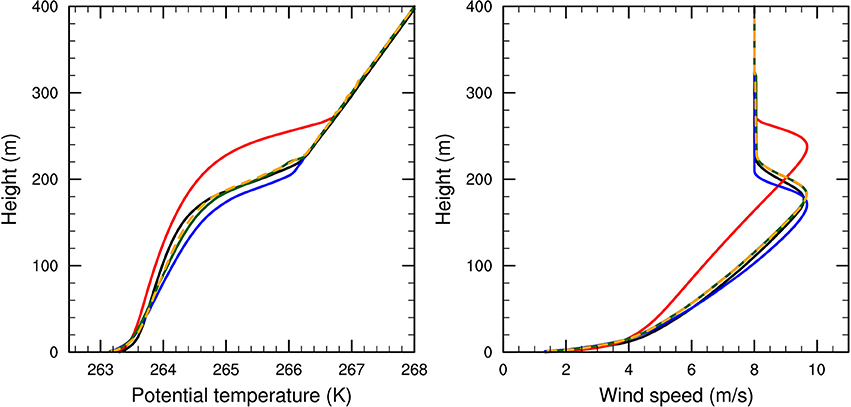
Figure 1. Mean potential temperature (Left) and wind speed (Right) averaged over the final hour (8–9th h) of the GABLS1 case: the LES with 2-m resolution (black), the reference SCM with the BL89 mixing length (red), the SCM with LES-forced L_m (blue), the SCM with LES-forced L_m and L_ϵ (green), and the SCM with LES-forced L_m, L_ϵ, and ψ_h (dashed orange).

In the L_m and L_ϵ (green) and the L_m, L_ϵ, and ψ_h (dotted orange) forced experiments, the mean profiles of the potential temperature and wind speed are closer to the LES than those of the SCM only forcing the mixing length. The forcing including ψ_h did not significantly improve the profiles because its value in this case is close to one. As expected, we see that including more LES-forced parameters produces results closer to those of the LES. However, the gains from the prescription of L_ϵ and ψ_h are much smaller than those from L_m alone, underlying the importance of the mixing length formulation.

3.2. Theoretical Formulation

Historically, the Prandtl formulation, l = κz (Prandtl, 1925), was predominantly used because it was known that turbulent structures are physically constrained by the distance to the ground. Later, the Blackadar estimation, l⁻¹ = (κz)⁻¹ + λ⁻¹, where λ is an asymptotic mixing length in the free atmosphere (Blackadar, 1962), added a limit imposed by neutral based observations. Various versions of the Blackadar mixing length with additional terms representing the stability effect have been proposed. For example, these additional terms include the Monin-Obukhov length (Delage, 1974) or the gradient Richardson number (Huang et al., 2013) defined by

$\begin{array}{ll}R{i}_g=\frac{N^2}{S^2}=\frac{\frac{g}{{\theta }_0}\frac{\partial \overline{\theta }}{\partial z}}{{\left(\frac{\partial \overline{U}}{\partial z}\right)}^2+{\left(\frac{\partial \overline{V}}{\partial z}\right)}^2},& (13)\end{array}$

which expresses counter effects of the inhibition of the turbulent motion via the static stability N and the production of turbulence via the vertical wind shear S. Other mixing length formulations are based only on the stability effect, such as the Deardorff formulation (Deardorff, 1980) described in Equation (2) or the BL89 formulation (Equation 6).

More recent studies have proposed mixing length formulations including the vertical wind shear effect. For example, Schumann and Gerz (1995) determined the momentum diffusivity K_m proportional to ϵ/S² with the dissipation of the TKE proportional to $\overline{{w\prime }^2}S$ (Hunt, 1988). Assuming $K_m=l\sqrt{e}$, the equivalent mixing length is expressed as

$\begin{array}{ll}l=\frac{1}{S}\frac{\overline{{w\prime }^2}}{\sqrt{e}}.& (14)\end{array}$

Similar formulation for the mixing length including only the vertical wind shear is proposed by Venayagamoorthy and Stretch (2010) from direct numerical simulations of homogeneous sheared turbulence :

$\begin{array}{ll}l=\frac{\sqrt{e}}{S},& (15)\end{array}$

which was tested in a parameterization of stably stratified turbulence by Wilson and Venayagamoorthy (2015). The shear length scale $\frac{\sqrt{e}}{S}$ was also combined with a buoyant length scale (Deardorff, 1980) for the study of a katabatic flow by Grisogono and Belušić (2008) such as :

$\begin{array}{ll}l=min\left(a\frac{\sqrt{e}}{N},b\frac{\sqrt{e}}{S}\right)& (16)\end{array}$

where a and b are constants. The additional shear length scale allowed to reduce the over-mixing of a buoyancy-based formulation in the z-less regime of the VSBL compared to an improved Prandtl model for a katabatic flow (Grisogono and Belušić, 2008; Grisogono, 2010). Although the representation of the length scales were improved recently for the SBL, a unifying formulation suitable for all stratification range is missing.

In Meso-NH, the reference length scale (Bougeault and Lacarrere, 1989) represents inaccurately the physical mixing in the stable and neutral boundary layers. For example in the GABLS1 case, Figure 1 shows that BL89 does not correctly represent the mixing in the SBL. Compared to LESs, the actual formulation of BL89 overestimates the turbulent mixing (as the old local buoyancy-based mixing length in Grisogono and Belušić, 2008). In stable conditions, the buoyancy term in the evolution of the TKE (Equation 3) becomes negative, so that dynamical production is the only remaining source of TKE. Therefore, the vertical wind shear effect is important. However, in the actual formulation of BL89, the wind shear is not represented. A possible solution to the overmixing prediction by BL89 within the SBL is to include the mean vertical wind shear S.

In a neutral atmosphere, physical mixing is not captured by BL89 because the term on the left-hand side of Equation (6) is zero. l_up extends to the top of the model in that case, which is physically not acceptable (see for example Section 3.3).

The primary goal of this study is to upgrade the current formulation to be physically more accurate for all stratification conditions. Dimensional arguments suggest modifying the length scales to be buoyancy-shear based (hereafter BS) such that

$\begin{array}{ll}\begin{array}{l}{\displaystyle {\int }_z^{z+l_{up}}}\left[\beta ({\theta }_v(z\prime )-{\theta }_v(z))+C_0\sqrt{e}S(z\prime )\right]dz\prime =e(z),\\ {\displaystyle {\int }_{z-l_{down}}^z}\left[\beta ({\theta }_v(z)-{\theta }_v(z\prime ))+C_0\sqrt{e}S(z\prime )\right]dz\prime =e(z),\end{array}& (17)\end{array}$

where C₀ is a constant and S(z′) is the local vertical wind shear.

The shear term corresponds to the slowdown effect produced by the vertical decoupling of turbulent structures when the local shear is strong (Figure 2). This effect also depends on the average eddy size, represented here by the TKE, because larger eddies are more decoupled. This new formulation is evaluated within the SCM Meso-NH on the simulated cases described in Section 2.2. The results are presented in Section 4.

FIGURE 2

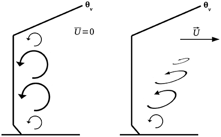
Figure 2. Schematic view of the effect of stratification and vertical wind shear on the reduction of the vertical mixing efficiency. Without wind shear (Left), the turbulent structures are constrained by the distance to the surface and by the stratification. The presence of a wind shear (Right) results in the stretching and decoupling of the turbulent structures.

3.3. Calibration of the Constant

The derivation of the constant C₀ of the proposed mixing length BS (Equation 17) is discussed in this section. To simplify the problem, it is possible to reduce the original formulation of BS in neutral conditions, where θ_v is vertically uniform, and assuming a constant wind shear, to

$\begin{array}{ll}\begin{array}{l}{\displaystyle {\int }_z^{z+l_{up}}}\left[C_0\sqrt{e}S\right]dz\prime =e(z),\\ {\displaystyle {\int }_{z-l_{down}}^z}\left[C_0\sqrt{e}S\right]dz\prime =e(z),\end{array}& (18)\end{array}$

which gives

$\begin{array}{ll}{l}_{up}=l_{down}=L_m=\frac{1}{C_0}\frac{\sqrt{e}}{S}.& (19)\end{array}$

Therefore, a neutral LES is performed in the configuration of Drobinski et al. (2007). The calibration of the constant C₀ is performed with two simulations of a neutral atmosphere with different geostrophic wind speeds, U_g = [10, 20] m.s⁻¹ (N10 and N20, Table 1). The constant is fitted to obtain the best agreement between the reference length L_K and the diagnosed BS (Equation 17) for the two neutral LESs. Here, we find C₀ = 0.50.

From the literature, it is possible to verify the consistency of the value of C₀ with previous studies. Wilson and Venayagamoorthy (2015) proposed in a shear-based parameterization the length scale L_K = cL_S, where L_S is defined in Equation (15) and c is the stress intensity ratio given by

$\begin{array}{ll}{c}^2=\frac{\sqrt{{\overline{u\prime w\prime }}^2+{\overline{v\prime w\prime }}^2}}{e}=\frac{\tau }{e},& (20)\end{array}$

where τ is the turbulent stress. Historically, the value of c² has been considered constant. For example, c = 0.52 was derived by Nieuwstadt (1984) from observations of near neutral stability during the Cabauw experiment (Driedonks et al., 1978). While recent studies (Mauritsen et al., 2007; Wilson and Venayagamoorthy, 2015) have shown that the stress intensity ratio may vary as a function of Ri_g, the value of c in neutral stability of c₀ = 0.50 has been suggested by high-Reynolds-number direct numerical simulations and experimental data (Karimpour and Venayagamoorthy, 2014).

The combination of the simplified formulation of the new mixing length in neutral stratification and constant shear (Equation 19) and L_m = L_K/C_m gives

$\begin{array}{ll}{L}_m=\frac{1}{C_0}\frac{\sqrt{e}}{S}=\frac{L_K}{C_m}.& (21)\end{array}$

Introducing the turbulent stress τ into the length scale L_K (Equation 10) results in

$\begin{array}{ll}{L}_K=\frac{\tau }{\sqrt{e}S},& (22)\end{array}$

which transforms Equation (21) into

$\begin{array}{ll}\frac{1}{C_0}\frac{\sqrt{e}}{S}=\frac{1}{C_m}\frac{\tau }{\sqrt{e}S}& (23)\end{array}$

and simplifies (using Equation 20) in a neutral atmosphere to

$\begin{array}{ll}\frac{C_m}{C_0}=\frac{\tau }{e}=c_0^2.& (24)\end{array}$

Here C_m = 0.126 and C₀ = 0.5 results in $c_0^2\approx 0.25$, which is in agreement with previous studies.

3.4. Verification of the Calibration with LESs

The proposed formulation is first directly evaluated in neutral and stable LESs. Figure 3 shows a comparison between the reference mixing length L_K/C_m (Equation 10), the current length scale BL89 (Equation 6), and the new length scale BS (Equation 17 with C₀ = 0.5) as diagnosed from the LES results. The mean profiles are averaged over the final hour of the simulation for the stably stratified cases and over the final 15 h for the neutrally stratified cases. A clear overestimation of the BL89 length (red curve) compared to the reference length scale (black) is seen for all cases. In the neutrally stratified cases, N10 and N20, BL89 results in a hyperbolic curve that is very different from the reference curve. This behavior is obviously not physically acceptable because the BL89 length is only influenced by the distance to the model boundaries. The reference length has an asymptotic value of ~300 m, regardless of the geostrophic wind. An asymptotic value for neutral mixing is usually observed (Blackadar, 1962). For the stably stratified cases, the mixing length has a maximum value near 0.2–0.3 the stable boundary-layer height (z_i, defined in Section 4.2). The new diagnosed length scale BS is in better agreement with the reference length for all simulated cases. Further evaluations of the new length scale are performed online in single-column simulations. Comparisons with the LES results are shown in the next section.

FIGURE 3

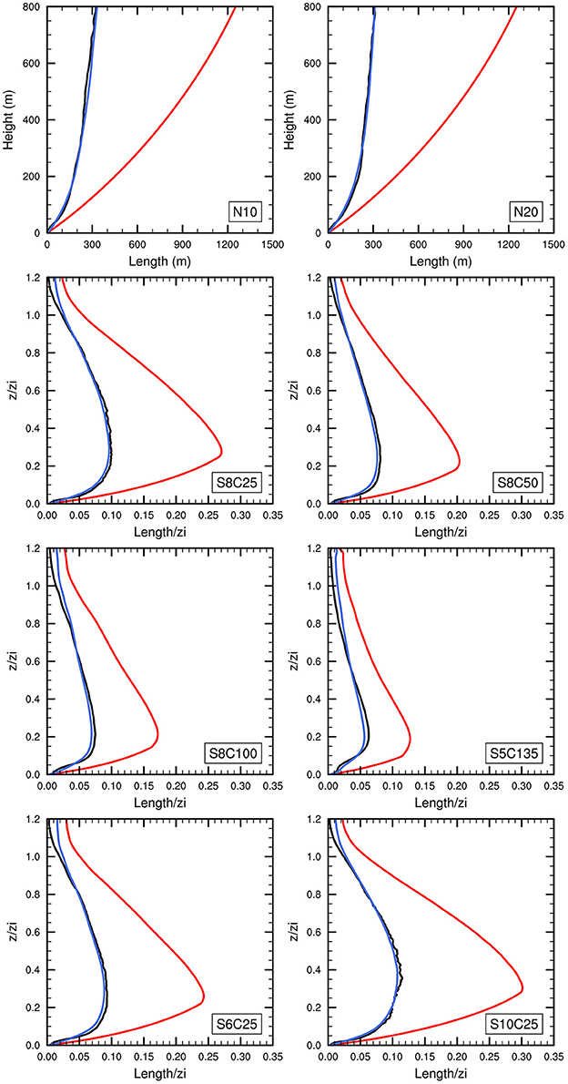
Figure 3. Mixing length L_m profiles from neutrally stratified (weak N10 and strong N20 geostrophic wind speed, see Table 1) and stably stratified (S8C25, S8C50, S8C100: weak to strong surface cooling; S6C25 and S10C25: weak to strong geostrophic wind speed; S5C135 weak geostrophic wind speed and strong surface cooling; see Table 1) LESs: the reference length L_K/C_m from Equation (10) (black), the diagnosed BL89 length (red), and the diagnosed BS length (blue). Profiles are scaled by the boundary-layer height z_i, except for the neutral atmospheres (N10 and N20).

4. Evaluation of Single-Column Simulations with Large-Eddy Simulations

4.1. Revisit of Model Constant

Single-column simulations of the stable and convective boundary-layers with the original BL89 and new mixing lengths BS are performed and compared to LESs. From preliminary tests, it was shown that the dissipation rate of the TKE was overestimated (not shown) and that a calibration of the dissipation constant C_ϵ (see Equation 1) needs to be made to maintain consistency with the new mixing length BS and the LES results.

In a neutral sheared flow along the x-axis, one assumes that a quasi-equilibrium between the production and dissipation of TKE can be reached. This is possible if, after initialization, the production of TKE is greater than its dissipation, which from the prognostic equation of the TKE (Equation 3) leads to the following condition:

$\begin{array}{ll}-\overline{u\prime w\prime }\frac{\partial \overline{U}}{\partial z}>ϵ.& (25)\end{array}$

Combining the expressions for the momentum flux and the diffusivity (Equations 4–5) and the dissipation rate of the TKE (Equation 1) leads to an expression for the mixing length, such that

$\begin{array}{ll}{L}_m^2>\frac{C_{ϵ}}{C_m}\frac{e}{{\left(\frac{\partial \overline{U}}{\partial z}\right)}^2}.& (26)\end{array}$

Combining Equation (26) and the expression for the new mixing length BS in neutral conditions (Equation 19), one can obtain a restriction on the constant C₀ such that

$\begin{array}{ll}{C}_0<\sqrt{\frac{C_m}{C_{ϵ}}}.& (27)\end{array}$

Derived from the neutrally stratified boundary layer (Section 3.3), C₀ = 0.5 is not in agreement with the current values of the model constants C_m and C_ϵ, which Equation (27) lead to C₀ < 0.385. One way to be consistent with the value of C₀ is to correct the dissipation constant C_ϵ.

The results from all LESs of neutrally and stably stratified cases also support a modification of the dissipation constant. Figure 4 shows the dispersion, at different times, of C_ϵ diagnosed from Equation (1) with respect to the gradient Richardson number (Equation 13). The dissipation length L_ϵ is evaluated using L_K/C_m (Equation 10) assuming L_ϵ = L_m. Data from neutral LESs collapse to Ri_g = 0 and show a large dispersion with a mean value lower than the currently used value of C_ϵ = 0.85 (Figure 4). In stably stratified cases, data are much more linearly dependent on the stability. This suggests that the commonly used assumption of L_ϵ = L_m may not be applicable, especially in stable flows. A discussion on this aspect is beyond the scope of this study. For simplicity, we correct the dissipation constant based on the mean value of all the neutral and stable LESs in this study (Figure 4), which is C_ϵ = 0.34. This value is used in the evaluation of the new length scale within the single-column simulations.

FIGURE 4

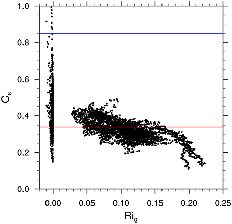
Figure 4. TKE dissipation constant C_ϵ computed by Equation (1) as a function of the gradient Richardson number (Equation 13) from neutrally stratified (N10 and N20) and stably stratified (S8C25, S8C50, S8C100, S5C135, S6C25, and S10C25; see Table 1) LESs. Horizontal lines represent the current constant value of C_ϵ = 0.85 (blue) and the new value of C_ϵ = 0.34 (red) estimated as the mean of all data.

4.2. Stable Boundary Layers

The new length scale is evaluated online in single-column simulations of a SBL. We compare the LES results to the single-column simulations with either the current mixing length, BL89, or the new proposed mixing length BS. The impacts of the new formulation for varying surface cooling and wind shear on the low-order moments and turbulent fluxes are discussed.

Figure 5 depicts the boundary-layer height z_i computed as

$\begin{array}{ll}\tau (z_{0.95})=0.05{\tau }_{surf.};z_i=z_{0.95}/0.95,& (28)\end{array}$

which corresponds to the height where the mean stress falls to 5% of its surface value followed by a correction via a linear extrapolation. This definition was proposed in the intercomparison GABLS1 (Kosovic and Curry, 2000; Beare et al., 2006; Cuxart et al., 2006) and has been used by other studies (e.g., Huang and Bou-Zeid, 2013). With this method, the boundary-layer height coincides with the LLJ altitude. For each stably stratified case (Table 1), the boundary-layer height reaches a quasi-steady state in 4–5 h (Figure 5). The LES results can be compared to other studies for the reference setup S8C25 (GABLS1); the present LES gives z_i ≈ 165 m, which is comparable to the range of LESs from Beare et al. (2006) ([149–164 m] at 1-m resolution and [162–197 m] at 2-m resolution) and the LES from Huang and Bou-Zeid (2013) (158 m). The impact of increasing surface cooling is a decrease in the surface wind stress leading to a shallower boundary layer (Figure 5). Increasing the cooling rate by 4 (Cr = [0.25, 1.0] K.h⁻¹) leads to a decrease in the boundary-layer height by 51% to 81 m. The impact of increasing (decreasing) the geostrophic wind is an increase (decrease) in the dynamical production of turbulent fluxes by the wind shear and, therefore, the boundary-layer height (Figure 5, S10C25 and S6C25 cases). Driven by weak wind and strong surface cooling, the case S5C135 has an extremely shallow SBL (Figure 5), on the order of the magnitude of that observed at Dome C, Antarctica (Bazile et al., 2015).

FIGURE 5

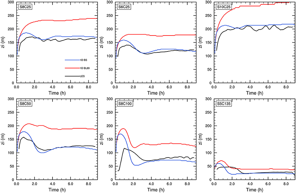
Figure 5. Time evolution of the boundary-layer height z_i (Equation 28) for the stably stratified cases (S8C25, S8C50, S8C100, S5C135, S6C25, and S10C25; see Table 1) for the LESs (black), the SCMs with the BL89 length (red), and the SCMs with the BS length (blue). For the LESs, the data are smoothed by a moving average.

In all cases, the boundary-layer height is overestimated by the SCM with the BL89 mixing length (Figure 5). The overestimation is ~35–52%. The use of the new BS length scale leads to a better prediction of the boundary-layer height compared to that of the LES. The reduction of the mixing length by the new formulation (see Section 3.4) induces a reduction of the turbulent fluxes, which leads to a lower boundary-layer height compared to that of the SCM with BL89.

An inspection of the final potential temperature and wind profiles (Figures 6, 7) demonstrates the sensitivity to varying surface cooling and geostrophic wind forcing. With a fixed cooling rate, the sensitivity to wind shear is shown with cases S6C25, S8C25, and S10C25. Increasing the geostrophic wind leads to an increase in the wind shear, enhancing turbulent mixing and, therefore, leading to a more curved potential temperature profile (Figure 6). With a fixed geostrophic wind, an increase in the surface cooling (S8C25, S8C50, and S8C100; note that the x-axes are not the same) leads to an enhancement in the vertical temperature gradient (Figure 6). A stronger stratification induces a stronger negative buoyancy flux (not shown), which reduces the turbulent mixing leading to a shallower SBL (Figure 5). The VSBL driven by the weak wind and strong surface cooling (S5C135) results in an extreme potential temperature gradient of ~0.3 K.m⁻¹ near the surface (Figure 6). Aloft, a much weaker temperature gradient is simulated by the LESs, especially in the more stable cases (S8C50, S8C100, and S5C135). This division of the SBL, into a strongly stable layer near the surface and a weaker stable layer above, was also simulated by Sullivan et al. (2016) for the stronger surface cooling rates; which is consistent with multi-layers structures of the VSBL (Smedman, 1988).

FIGURE 6

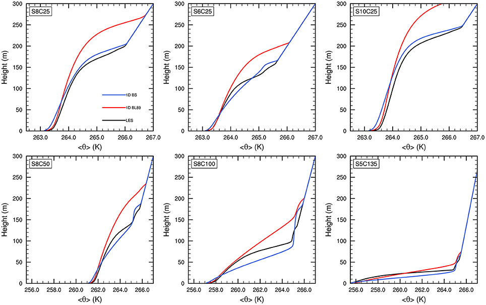
Figure 6. Potential temperature profiles averaged over the final hour (8–9th h) for the stably stratified cases (S8C25, S8C50, S8C100, S5C135, S6C25, and S10C25; see Table 1) for the LESs (black), the SCMs with the BL89 length (red), and the SCMs with the BS length (blue).

FIGURE 7

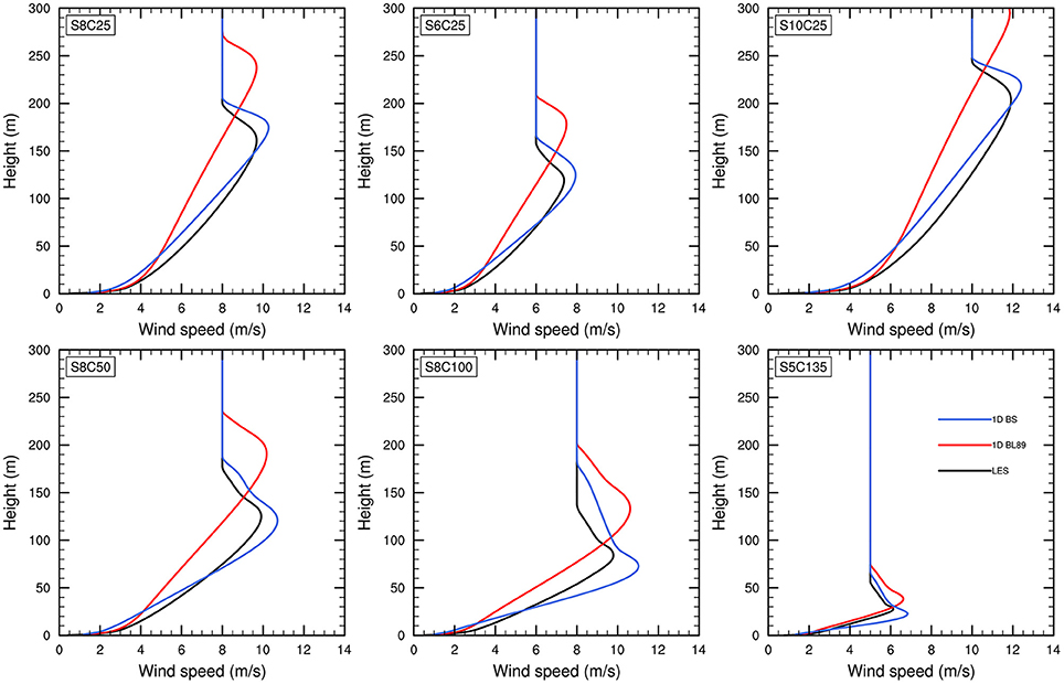
Figure 7. Wind speed profiles averaged over the final hour (8–9th h) for the stably stratified cases (S8C25, S8C50, S8C100, S5C135, S6C25, and S10C25; see Table 1) for the LESs (black), the SCMs with the BL89 length (red), and the SCMs with the BS length (blue).

Figure 7 shows the mean wind profiles for the final hour of the simulations. Increasing geostrophic wind forcing with fixed surface cooling [S6C25, S8C25, and S10C25] leads to a higher and stronger LLJ. Conversely, weaker geostrophic wind speeds tend to result in sharper LLJs (Blackadar, 1957). Increasing surface cooling with fixed geostrophic wind [S8C25, S8C50, and S8C100] also modifies the LLJ, which is sharper and at a lower level (Figure 7). For example, the LES S8C25 has its maximum wind speed at ~161 m while the 4 times higher surface cooling of S8C100 results in an LLJ at 84 m. The VSBL, S5C135, has a very low LLJ at ~27 m (Figure 7).

The overestimation of the turbulent mixing with BL89 in stably stratified cases is observed in the potential temperature and wind speed profiles. The SCM with BL89 overestimates the altitude of the LLJ and the slope of the wind profile in the lower part of the boundary layer (Figure 7). Overmixing is also associated with a more curved potential temperature profile (Grisogono, 2010) compared to that of the LES (Figure 6). The modified mixing length is in better agreement with that of the LES, with a less curved temperature profile, as well as a more realistic slope of the wind profile and altitude of the jet in all cases. Figure 8 illustrates a comparison between the LES and SCM for the position and strength of the LLJ in the six stably stratified cases. The intensity of the LLJ is slightly overestimated by the SCM compared to the LES depending on the case (Figure 8). In all simulated cases, the new SCM improves the predicted altitude of the maximum wind speed and the curvature of the potential temperature profile. Including the vertical wind shear explicitely in the mixing length reduces the over-diffusion in the SBL as found in Grisogono (2010) with a local formulation (Equation 16).

FIGURE 8

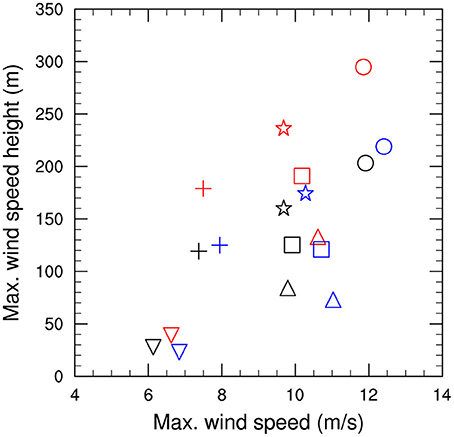
Figure 8. Height of the maximum wind speed as a function of the maximum wind speed value computed from the wind speed profile of the stably stratified cases (▽, S5C135; +, S6C25; , S8C25, □, S8C50; △, S8C100; and ○, S10C25; see Table 1) for the LESs (black), the SCMs with the BL89 length (red), and the SCMs with the BS length (blue).

To quantitatively compare the models performances between the LES and SCM, we use the integrated cooling (IC) of the boundary layer, as proposed by Steeneveld et al. (2006), given by

$\begin{array}{ll}IC={\displaystyle {\int }_{z=0}^{z=z_{TOP}}}\left[{\theta }_{final}(z)-{\theta }_{start}(z)\right]dz,& (29)\end{array}$

where z_TOP is the top of the model domain. The ICs of all the stably stratified cases are represented in Figure 9. The overestimation of the turbulent mixing with BL89 in the stably stratified cases induces stronger ICs compared to those in LESs (Figure 9). For comparison, Steeneveld et al. (2006) found an IC of −342 K.m using a first-order turbulence closure (Duynkerke, 1991, 1999) for the GABLS1 case (S8C25). In this study, the original SCM also gives a strong value of −366 K.m compared to that of the LES (−223 K.m; Figure 9). The SCM with the new length scale BS gives values better in agreement with that of the LES (Figure 9). Compared to those in LESs, the absolute IC amounts are larger for weak stable cases (S8C25 and S10C25) and smaller for stronger stable cases (S8C50, S8C100, and S5C135; Figure 9). A possible cause of this is the stability dependence of the dissipation constant (Figure 4), which is not included in the SCM. For example, the corrected value of C_ϵ = 0.34, used with the new length scale, is maybe too large compared to the LES-derived C_ϵ values for all data associated with Ri_g > 0.15 (Figure 4), i.e., for the strongest stratified cases (e.g., S8C100 and S5C135). Too much dissipation rate of the TKE induces too weak turbulent mixing which leads to warmer layers (Figure 6). The ICs are weaker compared to those of LESs (Figure 9), especially for the VSBL (S5C135) in which the original model with BL89 performs better than the new one in term of IC.

FIGURE 9

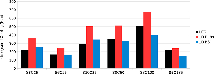
Figure 9. Integrated cooling (Equation 29) between the start and the end of the simulations for the stably stratified cases (S8C25, S8C50, S8C100, S5C135, S6C25, and S10C25; see Table 1) performed by the reference LESs, the original SCM (1D BL89), and the modified SCM with the new length scale (1D BS).

4.3. Convective Boundary Layers

The new length scale proposed in this study was originally motivated by the need for a better representation of the SBL. However, it is also important to verify the consistency of the new formulation in convective conditions. Two LESs of convective boundary layers (CBL) based on observations are reproduced as references with the model Meso-NH (for more information, see the description in Section 2.2.3). Again, the new length scale BS is evaluated in single-column mode by comparing the reference LES and 1D simulations with the current mixing length BL89.

For the two cases, the evolution of the potential temperature profiles is shown in Figure 10. The same initial profile is prescribed for the LESs and the single-column simulations; however, the initial profiles are very different between 05WC and IHOP. Case 05WC starts from a CBL with a weak capping inversion at ~1,000 m (Figure 10). IHOP starts from an initially stably stratified profile. Driven by different surface heat flux values, the CBL grows and reaches ~1,500 m for the 05WC LES and ~1,250 m for the IHOP LES after 7 h (similar to Figure 8 in Couvreux et al., 2005). For each case, after 7 h, the SCM underestimates the inversion height by ~200 m (Figure 10). The inversion is also much sharper than that in the explicit simulations. These features are observed when using the current and the new length scales in the single-column simulations. The new length scale shows nearly no impact on the potential temperature profile (Figure 10), which is unsurprising because the turbulent structures are primarily driven by the buoyancy force in convective conditions.

FIGURE 10

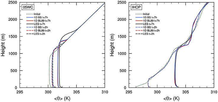
Figure 10. Potential temperature profiles for the convective cases with strong shear 05WC (Left) and weak shear IHOP (Right); see Table 1. Three runs are compared: the LES (black), the SCM with the BL89 length (red), and the SCM with the BS length (blue). Profiles are plotted 2 h (dashed line) and 7 h (solid line) after the start of the simulation (dotted line).

The modification of the turbulence scheme can be observed in the TKE profiles (Figure 11). For LESs, the sum of the resolved and subgrid TKEs is considered. In the 05WC LES, the initial convective stratification leads to strong mixing within the CBL, especially near the surface after 2 h (Figure 11). A vertical redistribution of the energy is observed after 7 h with much more TKE at the top of the CBL and less energy near the surface. This behavior is also captured in the single-column simulations. The use of the new length scale combined with the revisited dissipation constant leads to an increase in the TKE at each height compared to the reference SCM for both cases (Figure 11). This can be partially explained by the decrease in the dissipation constant, which decreases the dissipation rate of the TKE, as can be seen in the TKE budget (not shown). The less intense dissipation is balanced by the effect of the wind shear on the mixing length, which decreases the production of turbulent fluxes. The net effect is positive because the buoyancy effect in the new length scale formulation (Equation 17) is relatively much larger than the shear effect in convective conditions. Therefore, the reduction of the TKE production is small compared to the reduction of the dissipation rate of the TKE. With the current SCM, the TKE profiles are underestimated at each height compared to the LES profiles (Figure 11). The new model increases the turbulent mixing and conserves the shape of the TKE profile compared to the current model. However, the TKE is overestimated in the lower part of the CBL and underestimated in the upper part (Figure 11). To quantify the overall TKE profile within the CBL, we propose using the vertically integrated TKE computed within the first 2,000 m such that

$\begin{array}{ll}ITKE={\displaystyle {\int }_{z=0}^{z=2000m}}e(z\prime )dz\prime .& (30)\end{array}$

The current model underestimates the ITKE simulated by LESs by ~50% for each case (Figure 12). The new model improves the overall TKE within the CBL by a factor 4 in the root-mean square deviation of the ITKE for the IHOP and 05WC cases in the 2- and 7-h profiles.

FIGURE 11

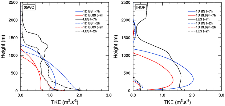
Figure 11. TKE profiles for the convective cases with strong shear 05WC (Left) and weak shear IHOP (Right); see Table 1. Three runs are compared: the LES (black), the SCM with the BL89 length (red), and the SCM with the BS length (blue). Profiles are plotted 2 (dashed line) and 7 h (solid line) after the start of the simulation (dotted line).

FIGURE 12

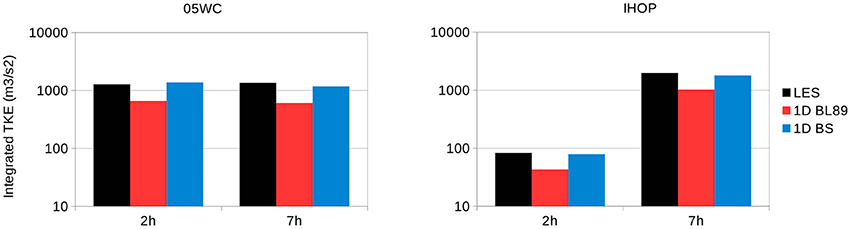
Figure 12. Vertically integrated TKE (Equation 30) for the convective cases with strong shear 05WC (Left) and weak shear IHOP (Right); see Table 1. Three runs are compared: the reference LESs, the original SCM (1D BL89), and the modified SCM with the new length scale (1D BS). The ITKE are computed 2 and 7 h after the start of the simulation.

5. Conclusions

In this study, a modified formulation for the mixing length in a TKE-l turbulence scheme was evaluated using large-eddy simulations (LESs) of stable and unstable stratified atmospheres. The new formulation integrates the local vertical wind shear within the non-local buoyancy-based formulation originally proposed by Bougeault and Lacarrere (1989). The integration of the wind shear is important in the representation of the mixing intensity especially in stably stratified flows because it is the only source of turbulence production.

Following the first model intercomparison GEWEX Atmospheric boundary layer Study (GABLS1; Beare et al., 2006; Cuxart et al., 2006), the GABLS1 case was reproduced using the model Meso-NH, which can be used in LES and single-column modes. This idealized case of a weakly stably stratified boundary layer has the advantage of being primarily driven by turbulent mixing because the surface cooling and geostrophic wind are prescribed. A numerical experiment was performed where the single-column model (SCM) was forced by LES-derived turbulent parameters (the mixing L_m and dissipation L_ϵ lengths and the stability function for heat ψ_h). This experiment highlighted the importance of the mixing length formulation.

We also demonstrated the importance of revisiting the dissipation constant C_ϵ for the SCM. It is clear that there is a need to include a stability correction in the dissipation length scale (see for example Redelsperger et al., 2001) instead of using the traditional assumption of L_m = L_ϵ. The commonly used expression for the dissipation rate of the TKE (Equation 1) should be modified, especially in stable conditions where the motions are not isotropic. This deserves further study.

The new mixing length formulation was tested on neutrally stratified cases with different shear conditions, various stably stratified cases with varying surface cooling and geostrophic wind, and two convective cases. For stably stratified atmospheres, the new turbulence scheme is in better agreement with LESs in terms of turbulent mixing, the low-level jet and boundary-layer heights, and the temperature inversion. The overestimation of turbulent mixing in stably stratified atmosphere, a consequence of the current mixing length, was overcome by including the local vertical wind shear. For convective stratifications, the new SCM was evaluated against two cases (Ayotte et al., 1996; Couvreux et al., 2005). Because the wind shear is not the main driving process in the development of a convective boundary layer, a very slight impact of the new length scale was simulated, as expected. This indicates that the new buoyancy–shear mixing length can be used in weather prediction and atmospheric models for any type of stability condition.

Author Contributions

QR performed the numerical experiments and led the theoretical analysis of the study. VM and FC substantially contributed to the manipulation of the model and of the design of specific sections of the manuscript. All authors contributed on the comprehension of the question raised by the study, as well as on the revision and correction of the manuscript. Agreement to be accountable for all aspects of the work in ensuring that questions related to the accuracy or integrity of any part of the work were appropriately investigated and resolved by all authors.

Conflict of Interest Statement

The authors declare that the research was conducted in the absence of any commercial or financial relationships that could be construed as a potential conflict of interest.

Supplementary Material

The Supplementary Material for this article can be found online at: https://www.frontiersin.org/article/10.3389/feart.2017.00065/full#supplementary-material

References

Ayotte, K. W., Sullivan, P. P., Andrén, A., Doney, S. C., Holtslag, A. A., Large, W. G., et al. (1996). An evaluation of neutral and convective planetary boundary-layer parameterizations relative to large eddy simulations. Boundary Layer Meteorol. 79, 131–175. doi: 10.1007/BF00120078

CrossRef Full Text | Google Scholar

Banta, R. (2008). Stable-boundary-layer regimes from the perspective of the low-level jet. Acta Geophys. 56, 58–87. doi: 10.2478/s11600-007-0049-8

CrossRef Full Text | Google Scholar

Bazile, E., Couvreux, F., and Le Moigne, P. (2015). “The gabls4 inter-comparison: preliminary results,” in 2015 AGU Fall Meeting. San Francisco, CA: Agu.

Google Scholar

Beare, R. J., and Macvean, M. K. (2004). Resolution sensitivity and scaling of large-eddy simulations of the stable boundary layer. Boundary layer Meteorol. 112, 257–281.

Google Scholar

Beare, R. J., Macvean, M. K., Holtslag, A. A., Cuxart, J., Esau, I., Golaz, J.-C., et al. (2006). An intercomparison of large-eddy simulations of the stable boundary layer. Boundary Layer Meteorol. 118, 247–272. doi: 10.1007/s10546-004-2820-6

CrossRef Full Text | Google Scholar

Beljaars, A., Balsamo, G., Betts, A., Dutra, E., Ghelli, A., Köhler, M., et al. (2012). “The stable boundary layer in the ecmwf model,” in Proceedings of ECMWF Workshop on Diurnal Cycles and the Stable Boundary Layer (Reading: ECMWF/WCRP), 1–10.

Google Scholar

Blackadar, A. K. (1957). Boundary layer wind maxima and their significance for the growth of nocturnal inversions. Bull. Amer. Meteor. Soc. 38, 283–290.

Google Scholar

Blackadar, A. K. (1962). The vertical distribution of wind and turbulent exchange in a neutral atmosphere. J. Geophys. Res. 67, 3095–3102. doi: 10.1029/JZ067i008p03095

CrossRef Full Text | Google Scholar

Bosveld, F. C., Baas, P., Steeneveld, G.-J., Holtslag, A. A., Angevine, W. M., Bazile, E., et al. (2014). The third gabls intercomparison case for evaluation studies of boundary-layer models. part b: results and process understanding. Boundary-Layer Meteorol. 152, 157–187. doi: 10.1007/s10546-014-9919-1

CrossRef Full Text | Google Scholar

Bougeault, P., and Lacarrere, P. (1989). Parameterization of orography-induced turbulence in a mesobeta–scale model. Month. Weather Rev. 117, 1872–1890. doi: 10.1175/1520-0493(1989)117<1872:POOITI>2.0.CO;2

CrossRef Full Text | Google Scholar

Brost, R., and Wyngaard, J. (1978). A model study of the stably stratified planetary boundary layer. J. Atmospher. Sci. 35, 1427–1440. doi: 10.1175/1520-0469(1978)035<1427:AMSOTS>2.0.CO;2

CrossRef Full Text | Google Scholar

Businger, J. A., Wyngaard, J. C., Izumi, Y., and Bradley, E. F. (1971). Flux-profile relationships in the atmospheric surface layer. J. Atmospher. Sci. 28, 181–189. doi: 10.1175/1520-0469(1971)028<0181:FPRITA>2.0.CO;2

CrossRef Full Text | Google Scholar

Cheng, Y., Canuto, V., and Howard, A. (2002). An improved model for the turbulent pbl. J. Atmospher. Sci. 59, 1550–1565. doi: 10.1175/1520-0469(2002)059<1550:AIMFTT>2.0.CO;2

CrossRef Full Text | Google Scholar

Couvreux, F., Guichard, F., Redelsperger, J.-L., Kiemle, C., Masson, V., Lafore, J.-P., et al. (2005). Water-vapour variability within a convective boundary-layer assessed by large-eddy simulations and ihop_2002 observations. Q. J. R. Meteorol. Soc. 131, 2665–2693. doi: 10.1256/qj.04.167

CrossRef Full Text | Google Scholar

Cuxart, J., Bougeault, P., and Redelsperger, J.-L. (2000). A turbulence scheme allowing for mesoscale and large-eddy simulations. Q. J. R. Meteorol. Soc. 126, 1–30. doi: 10.1002/qj.49712656202

CrossRef Full Text | Google Scholar

Cuxart, J., Holtslag, A. A., Beare, R. J., Bazile, E., Beljaars, A., Cheng, A., et al. (2006). Single-column model intercomparison for a stably stratified atmospheric boundary layer. Boundary-Layer Meteorol. 118, 273–303. doi: 10.1007/s10546-005-3780-1

CrossRef Full Text | Google Scholar

Deardorff, J. W. (1980). Stratocumulus-capped mixed layers derived from a three-dimensional model. Boundary-Layer Meteorol. 18, 495–527. doi: 10.1007/BF00119502

CrossRef Full Text | Google Scholar

Delage, Y. (1974). A numerical study of the nocturnal atmospheric boundary layer. Q. J. R. Meteorol. Soc. 100, 351–364. doi: 10.1002/qj.49710042507

CrossRef Full Text | Google Scholar

Driedonks, A., Van Dop, H., and Kohsiek, W. (1978). “Meteorological observations on the 213 m mast at cabauw, in the netherlands,” in 4th Symposium on Meteorological Observations and Instrumentation, vol. 1 (Denver, CO), 41–46.

Google Scholar

Drobinski, P., Carlotti, P., Newsom, R. K., Banta, R. M., Foster, R. C., and Redelsperger, J.-L. (2004). The structure of the near-neutral atmospheric surface layer. J. Atmospher. Sci. 61, 699–714. doi: 10.1175/1520-0469(2004)061<0699:TSOTNA>2.0.CO;2

CrossRef Full Text | Google Scholar

Drobinski, P., Carlotti, P., Redelsperger, J.-L., Masson, V., Banta, R. M., and Newsom, R. K. (2007). Numerical and experimental investigation of the neutral atmospheric surface layer. J. Atmospher. Sci. 64, 137–156. doi: 10.1175/JAS3831.1

CrossRef Full Text | Google Scholar

Duynkerke, P., and Driedonks, A. (1987). A model for the turbulent structure of the stratocumulus-topped atmospheric boundary layer. J. Atmospher. Sci. 44, 43–64. doi: 10.1175/1520-0469(1987)044<0043:AMFTTS>2.0.CO;2

CrossRef Full Text | Google Scholar

Duynkerke, P. G. (1991). Radiation fog: a comparison of model simulation with detailed observations. Month. Weather Rev. 119, 324–341. doi: 10.1175/1520-0493(1991)119<0324:RFACOM>2.0.CO;2

CrossRef Full Text | Google Scholar

Duynkerke, P. G. (1999). Turbulence, radiation and fog in dutch stable boundary layers. Boundary-Layer Meteorol. 90, 447–477. doi: 10.1023/A:1026441904734

CrossRef Full Text | Google Scholar

Dyer, A. (1974). A review of flux-profile relationships. Boundary Layer Meteorol. 7, 363–372. doi: 10.1007/BF00240838

CrossRef Full Text | Google Scholar

Grisogono, B. (2010). Generalizing ‘z-less’ mixing length for stable boundary layers. Q. J. R. Meteorol. Soc. 136, 213–221. doi: 10.1002/qj.529

CrossRef Full Text | Google Scholar

Grisogono, B., and Belušić, D. (2008). Improving mixing length-scale for stable boundary layers. Q. J. R. Meteorol. Soc. 134, 2185–2192. doi: 10.1002/qj.347

CrossRef Full Text | Google Scholar

Grisogono, B., and Enger, L. (2004). Boundary-layer variations due to orographic-wave breaking in the presence of rotation. Q. J. R. Meteorol. Soc. 130, 2991–3014. doi: 10.1256/qj.03.190

CrossRef Full Text | Google Scholar

Hansen, K. S., Barthelmie, R. J., Jensen, L. E., and Sommer, A. (2012). The impact of turbulence intensity and atmospheric stability on power deficits due to wind turbine wakes at horns rev wind farm. Wind Energy 15, 183–196. doi: 10.1002/we.512

CrossRef Full Text | Google Scholar

Holtslag, A., and Boville, B. (1993). Local versus nonlocal boundary-layer diffusion in a global climate model. J. Climate 6, 1825–1842. doi: 10.1175/1520-0442(1993)006<1825:LVNBLD>2.0.CO;2

CrossRef Full Text | Google Scholar

Holtslag, A., Svensson, G., Baas, P., Basu, S., Beare, B., Beljaars, A., et al. (2013). Stable atmospheric boundary layers and diurnal cycles: challenges for weather and climate models. Bull. Amer. Meteorol. Soc. 94, 1691–1706. doi: 10.1175/BAMS-D-11-00187.1

CrossRef Full Text | Google Scholar

Holtslag, B. (2006). Preface: gewex atmospheric boundary-layer study (gabls) on stable boundary layers. Boundary Layer Meteorol. 118, 243–246. doi: 10.1007/s10546-005-9008-6

CrossRef Full Text | Google Scholar

Hourdin, F., Grandpeix, J.-Y., Rio, C., Bony, S., Jam, A., Cheruy, F., et al. (2013). Lmdz5b: the atmospheric component of the ipsl climate model with revisited parameterizations for clouds and convection. Climate Dyn. 40, 2193–2222. doi: 10.1007/s00382-012-1343-y

CrossRef Full Text | Google Scholar

Huang, J., and Bou-Zeid, E. (2013). Turbulence and vertical fluxes in the stable atmospheric boundary layer. Part I: a large-eddy simulation study. J. Atmospher. Sci. 70, 1513–1527. doi: 10.1175/JAS-D-12-0167.1

CrossRef Full Text | Google Scholar

Huang, J., Bou-Zeid, E., and Golaz, J.-C. (2013). Turbulence and vertical fluxes in the stable atmospheric boundary layer. Part II: a novel mixing-length model. J. Atmospher. Sci. 70, 1528–1542. doi: 10.1175/JAS-D-12-0168.1

CrossRef Full Text | Google Scholar

Hunt, J. (1988). “Length scales in stably stratified turbulent flows and their use in turbulence models,” in Stably Stratified Flow and Dense Gas Dispersion, ed J. S. Puttock (Oxford, UK: Oxford University Press), 285–321.

Google Scholar

Karimpour, F., and Venayagamoorthy, S. K. (2014). A revisit of the equilibrium assumption for predicting near-wall turbulence. J. Fluid Mech. 760, 304–312. doi: 10.1017/jfm.2014.532

CrossRef Full Text | Google Scholar

Kolmogorov, A. N. (1941). Dissipation of energy in locally isotropic turbulence [in russian]. Dokl. Akad. Nauk SSSR. 32, 19–21.

Google Scholar

Kosovic, B., and Curry, J. A. (2000). A large eddy simulation study of a quasi-steady, stably stratified atmospheric boundary layer. J. Atmospher. Sci. 57, 1052–1068. doi: 10.1175/1520-0469(2000)057<1052:ALESSO>2.0.CO;2

CrossRef Full Text

Lafore, J. P., Stein, J., Asencio, N., Bougeault, P., Ducrocq, V., Duron, J., et al. (1998). “The meso-nh atmospheric simulation system. Part I: adiabatic formulation and control simulations,” in Annales Geophysicae, vol. 16, ed L. Eymard (Göttingen: Springer), 90–109.

Google Scholar

Lenderink, G., and Holtslag, A. A. (2004). An updated length-scale formulation for turbulent mixing in clear and cloudy boundary layers. Q. J. R. Meteorol. Soc. 130, 3405–3427. doi: 10.1256/qj.03.117

CrossRef Full Text | Google Scholar

Mahrt, L. (1998). Stratified atmospheric boundary layers and breakdown of models. Theor. Comput. Fluid Dyn. 11, 263–279. doi: 10.1007/s001620050093

CrossRef Full Text | Google Scholar

Mahrt, L. (2014). Stably stratified atmospheric boundary layers. Ann. Rev. Fluid Mech. 46, 23–45. doi: 10.1146/annurev-fluid-010313-141354

CrossRef Full Text | Google Scholar

Matheou, G., and Chung, D. (2014). Large-eddy simulation of stratified turbulence. Part II: application of the stretched-vortex model to the atmospheric boundary layer. J. Atmospher. Sci. 71, 4439–4460. doi: 10.1175/JAS-D-13-0306.1

CrossRef Full Text | Google Scholar

Mauritsen, T., Svensson, G., Zilitinkevich, S. S., Esau, I., Enger, L., and Grisogono, B. (2007). A total turbulent energy closure model for neutrally and stably stratified atmospheric boundary layers. J. Atmospher. Sci. 64, 4113–4126. doi: 10.1175/2007JAS2294.1

CrossRef Full Text | Google Scholar

Mellor, G. L., and Yamada, T. (1974). A hierarchy of turbulence closure models for planetary boundary layers. J. Atmospher. Sci. 31, 1791–1806. doi: 10.1175/1520-0469(1974)031<1791:AHOTCM>2.0.CO;2

CrossRef Full Text | Google Scholar

Mellor, G. L., and Yamada, T. (1982). Development of a turbulence closure model for geophysical fluid problems. Rev. Geophys. 20, 851–875. doi: 10.1029/RG020i004p00851

CrossRef Full Text | Google Scholar

Monin, A., and Obukhov, A. (1954). Basic laws of turbulent mixing in the surface layer of the atmosphere. Contrib. Geophys. Inst. Acad. Sci. USSR 151:e187.

Google Scholar

Nieuwstadt, F. T. (1984). The turbulent structure of the stable, nocturnal boundary layer. J. Atmospher. Sci. 41, 2202–2216. doi: 10.1175/1520-0469(1984)041<2202:TTSOTS>2.0.CO;2

CrossRef Full Text | Google Scholar

Pergaud, J., Masson, V., Malardel, S., and Couvreux, F. (2009). A parameterization of dry thermals and shallow cumuli for mesoscale numerical weather prediction. Boundary Layer Meteorol. 132, 83–106. doi: 10.1007/s10546-009-9388-0

CrossRef Full Text | Google Scholar

Prandtl, L. (1925). Bericht über untersuchungen zur ausgebildeten turbulenz. Z. Angew. Math. Mech. 5, 136–139.

Google Scholar

Randall, D. A., Xu, K.-M., Somerville, R. J., and Iacobellis, S. (1996). Single-column models and cloud ensemble models as links between observations and climate models. J. Climate 9, 1683–1697. doi: 10.1175/1520-0442(1996)009<1683:SCMACE>2.0.CO;2

CrossRef Full Text | Google Scholar

Redelsperger, J., and Sommeria, G. (1982). Method of representing the turbulence associated with precipitations in a three-dimensional model of cloud convection. Boundary Layer Meteorol. 24, 231–252. doi: 10.1007/BF00121669

CrossRef Full Text

Redelsperger, J.-L., Mahé, F., and Carlotti, P. (2001). A simple and general subgrid model suitable both for surface layer and free-stream turbulence. Boundary Layer Meteorol. 101, 375–408. doi: 10.1023/A:1019206001292

CrossRef Full Text | Google Scholar

Redelsperger, J.-L., and Sommeria, G. (1986). Three-dimensional simulation of a convective storm: sensitivity studies on subgrid parameterization and spatial resolution. J. Atmospher. Sci. 43, 2619–2635. doi: 10.1175/1520-0469(1986)043<2619:TDSOAC>2.0.CO;2

CrossRef Full Text | Google Scholar

Schumann, U., and Gerz, T. (1995). Turbulent mixing in stably stratified shear flows. J. Appl. Meteorol. 34, 33–48. doi: 10.1175/1520-0450-34.1.33

CrossRef Full Text | Google Scholar

Seity, Y., Brousseau, P., Malardel, S., Hello, G., Bénard, P., Bouttier, F., et al. (2011). The arome-france convective-scale operational model. Month. Weather Rev. 139, 976–991. doi: 10.1175/2010MWR3425.1

CrossRef Full Text | Google Scholar

Smedman, A.-S. (1988). Observations of a multi-level turbulence structure in a very stable atmospheric boundary layer. Boundary Layer Meteorol. 44, 231–253. doi: 10.1007/BF00116064

CrossRef Full Text | Google Scholar

Steeneveld, G., Van De Wiel, B. J., and Holtslag, A. A. (2006). Modelling the arctic stable boundary layer and its coupling to the surface. Boundary Layer Meteorol. 118, 357–378. doi: 10.1007/s10546-005-7771-z

CrossRef Full Text | Google Scholar

Sullivan, P. P., Weil, J. C., Patton, E. G., Jonker, H. J., and Mironov, D. V. (2016). Turbulent winds and temperature fronts in large-eddy simulations of the stable atmospheric boundary layer. J. Atmospher. Sci. 73, 1815–1840. doi: 10.1175/JAS-D-15-0339.1

CrossRef Full Text | Google Scholar

Svensson, G., Holtslag, A. A., Kumar, V., Mauritsen, T., Steeneveld, G., Angevine, W., et al. (2011). Evaluation of the diurnal cycle in the atmospheric boundary layer over land as represented by a variety of single-column models: the second gabls experiment. Boundary Layer Meteorol. 140, 177–206. doi: 10.1007/s10546-011-9611-7

CrossRef Full Text | Google Scholar

Tjernström, M. (1993). Turbulence length scales in stably stratified free shear flow analyzed from slant aircraft profiles. J. Appl. Meteorol. 32, 948–963. doi: 10.1175/1520-0450(1993)032<0948:TLSISS>2.0.CO;2

CrossRef Full Text | Google Scholar

Van de Wiel, B., Moene, A., Hartogensis, O., De Bruin, H., and Holtslag, A. (2003). Intermittent turbulence in the stable boundary layer over land. Part III: a classification for observations during cases-99. J. Atmospher. Sci. 60, 2509–2522. doi: 10.1175/1520-0469(2003)060<2509:ITITSB>2.0.CO;2

CrossRef Full Text | Google Scholar

Venayagamoorthy, S. K., and Stretch, D. D. (2010). On the turbulent prandtl number in homogeneous stably stratified turbulence. J. Fluid Mech. 644, 359–369. doi: 10.1017/S002211200999293X

CrossRef Full Text | Google Scholar

Viterbo, P., Beljaars, A., Mahfouf, J.-F., and Teixeira, J. (1999). The representation of soil moisture freezing and its impact on the stable boundary layer. Q. J. R. Meteorol. Soc. 125, 2401–2426. doi: 10.1002/qj.49712555904

CrossRef Full Text | Google Scholar

Weil, J. C. (2012). Stable Boundary Layer Modeling for Air Quality Applications. Dordrecht: Springer.

Google Scholar

Wilson, J. M., and Venayagamoorthy, S. K. (2015). A shear-based parameterization of turbulent mixing in the stable atmospheric boundary layer. J. Atmospher. Sci. 72, 1713–1726. doi: 10.1175/JAS-D-14-0241.1

CrossRef Full Text | Google Scholar

Zilitinkevich, S., Elperin, T., Kleeorin, N., Rogachevskii, I., Esau, I., Mauritsen, T., et al. (2008). Turbulence energetics in stably stratified geophysical flows: Strong and weak mixing regimes. Q. J. R. Meteorol. Soc. 134, 793–799. doi: 10.1002/qj.264

CrossRef Full Text | Google Scholar