Considerations for Latitudinal Time-Averaged-Field Palaeointensity Analysis of the Last Five Million Years

Introduction

From geomagnetic observations and palaeomagnetic records, we know that the Earth's magnetic field is dominated by a dipole component, which is also dynamic and changing in terms of both its direction and intensity (Valet, 2003). Central to much palaeomagnetic research, e.g., palaeogeographic reconstructions, is the assumption that the time-averaged field (TAF) is a dipole field aligned parallel with the Earth's spin axis, the so-called geocentric-axial-dipole (GAD) hypothesis. Over very long periods of time, i.e., 200 million years, from palaeomagnetic directional data this hypothesis has been shown to hold (Merrill and McFadden, 2003); however, it has been known for some time (Wilson, 1970) that there are systematic departures from this simple model over shorter timescales. Direct field observations only encompass the last 400 years or so (Jackson et al., 2000), and reveal a strongly non-GAD field. If undetected, these non-GAD fields can have a major impact on palaeogeographical reconstructions creating spurious mismatches, for example, palaeomagnetic results from the timespan 0–5 Ma (Kono et al., 2000; Johnson et al., 2008) suggest a significant non-GAD contribution to the TAF of the order ~5% (mostly quadrupole and octupole) that can correspond to ~500 km reconstruction mismatches. Deviations from GAD are greatest at high-latitudes, but the exact nature and duration of these deviations is still debated (Constable, 2007). These high-latitudes deviations are greater in the ancient geomagnetic field intensity (palaeointensity) record than the directional record (Constable, 2007).

In the analysis of palaeointensity data as a function of latitude, it is common to plot palaeointensity data as a function of latitude for latitudinally binned “reliable” absolute palaeointensity data from the last 5 Myr using the PINT database (Biggin et al., 2009) available at http://earth.liv.ac.uk/pint; when binning the data sometimes the average of each bin is taken (e.g., Lawrence et al., 2009; Wang et al., 2015) and sometimes the median (e.g., Cromwell et al., 2015; Døssing et al., 2016). The definition of “reliable” varies between studies, but the same trend is observed: the measured intensity data deviates most from the GAD intensity model B^D at high latitudes, where B^D varies with the (magnetic) co-latitude θ by.

$\begin{array}{cc}{B}^D=B_{eq}^D{(1+3{\cos }^2\theta )}^{\frac{1}{2}}& (1)\end{array}$

where $B_{eq}^D$ is the field intensity at the equator for an axial dipole field.

If the geomagnetic field was a steady-state GAD field, then a plot of the binned palaeointensity data from the last 5 Myr against latitude should lead to a dipole field, however, we know from the current-day geomagnetic field that the field it is not a GAD and it displays secular variation. However, by comparing the GAD intensity model and the binned palaeointensity data against latitude, it is intrinsically assumed that a TAF has the possibility of resembling a GAD field. In this paper, by considering the contribution of secular variation to the geomagnetic field, I show that it is simply incorrect; comparing binned palaeointensity data against a dipole field aligned along the rotation axis leads to an overestimation which is greatest at high latitudes, i.e., it is not possible for a TAF to be a GAD field due to secular variation. However, including dipole secular variation, does not explain the data trend found in the PINT database (Biggin et al., 2009); I further then investigate how permanent non-dipole structures might explain the latitudinal discrepancy.

A Simple Cap Model for Dipolar Secular Variation

In studies that compare intensity vs. latitude (e.g., Lawrence et al., 2009; Cromwell et al., 2015; Wang et al., 2015; Døssing et al., 2016), it is the geographical latitude, not the palaeomagnetic latitude, that is used; this removes the circular logic of using GAD theory to calculate the palaeomagnetic latitude in a study of the robustness of the GAD hypothesis. Only palaeointensity data from the last 5 Myr are usually considered, because, as a first-order approximation, this removes the need to include any tectonic corrections to the sample locations' geographic latitudes. Once selected and latitudinally binned, the palaeointensity data are often directly compared to the intensity of the GAD field B^D Equation (1).

However, the field experienced at a sample location S is not a GAD field, but as a first-order approximation a dipole field with a pole position P (Figure 1). The position of the current-day dipole field pole drifts, i.e., westward drift, 360° around the rotation axis and geographic pole G, with a tilt angle of ~11°; the tilt angle also varies (Jackson et al., 2000; Constable, 2007). In determining the TAF intensity behavior of the palaeointensity database, we need to include secular variation of pole position P; it is simply incorrect to average all the data points from a given latitude as the field experienced at a given latitude depends on the magnetic co-latitude, which varies with time and depends on a cosine function of the co-latitude Equation (1).

FIGURE 1

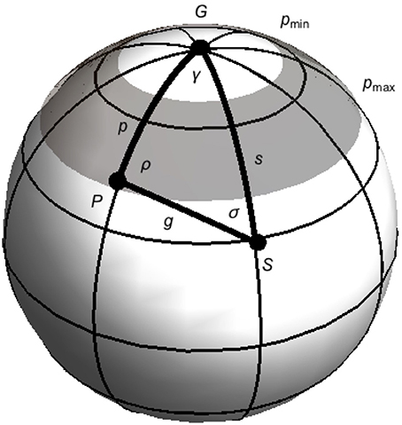
Figure 1. Schematic diagram showing the relationship between the geographic pole position G, a dipole pole position P and a sampling locality S. The three positions are connected by three great-circle arc-lengths p, s and g at angles ρ, γ, and σ as shown. Note the break from the standard naming convention for a triangle. The limits p_max and p_min are shown, with a corresponding integration surface for Equation (3) in gray.

To demonstrate the effect of latitude on dipolar secular variation, consider a simple cap model of dipolar secular variation: The average great-circle length between P and S, i.e., g (Figure 1), which equals the magnetic co-latitude on a unit-sphere. For a fixed sample location S, the arc-length g depends on both γ (westward drift) and tilt angle (arc-length p). γ varies between 0 and 360°, and the tilt-angle/arc-length p between p_min and p_max; if p_min = 0 the area is simply a cap. The average g for a point S can be determined using the Law of Cosines, which on a sphere with unit radius gives:

$\begin{array}{cc}\begin{array}{l}\overline{\cos g}=\frac{{\displaystyle \underset{p=p_{\min }}{\overset{p_{\max }}{\int }}{\displaystyle \underset{\gamma =0}{\overset{2\pi }{\int }}(\cos p\cos s+\sin p\sin s\cos \gamma )\sin pd\gamma }}dp}{{\displaystyle \underset{p=p_{\min }}{\overset{p_{\max }}{\int }}{\displaystyle \underset{\gamma =0}{\overset{2\pi }{\int }}\sin pd\gamma }}dp}\\ =\frac{\cos s}{4}\frac{(\cos 2p_{\min }-\cos 2p_{\max })}{(\cos p_{\min }-\cos p_{\max })}\end{array}& (2)\end{array}$

where $\overline{cosg}$ is the average cosg for the area under consideration.

To study the TAF, the palaeointensity data are binned from different time periods over intervals of typically 10–15° latitude (Wang et al., 2015; Døssing et al., 2016). The average of ${\overline{cosg}}_{s_{min}}^{s_{max}}$ over a sample latitude window s_min to s_max is simply given by:

$\begin{array}{cc}\begin{array}{l}{\overline{\cos g}}_{s_{\min }}^{s_{\max }}=\frac{{\displaystyle \underset{s=s_{\min }}{\overset{s_{\max }}{\int }}\left(\frac{\cos s}{4}\frac{(\cos 2p_{\min }-\cos 2p_{\max })}{(\cos p_{\min }-\cos p_{\max })}\right)}\sin sds}{{\displaystyle \underset{s=s_{\min }}{\overset{s_{\max }}{\int }}\sin }sds}\\ =\frac{1}{16}\frac{(\cos 2p_{\min }-\cos 2p_{\max })}{(\cos p_{\min }-\cos p_{\max })}\frac{(\cos 2s_{\min }-\cos 2s_{\max })}{(\cos s_{\min }-\cos s_{\max })}\end{array}& (3)\end{array}$

To calculate the time-averaged intensity B^TAF as a function of latitude for a dipole field that displays secular variation as recorded by latitudinally binned palaeointensity data, simply put Equation (3) into Equation (1) to give:

$\begin{array}{cc}{B}^{TAF}=B_{eq}^{TAF}{\left(1+3{\cos }^2{\overline{g}}_{s_{\min }}^{s_{\max }}\right)}^{\frac{1}{2}}& (4)\end{array}$

where ${\overline{g}}_{s_{min}}^{s_{max}}$ is the average of g determined from Equation (3) for a site-latitude window between s_min to s_max, and $B_{eq}^{TAF}$ is the field intensity at the equator for the TAF.

Using a latitudinal bin size of 10°, I have calculated Equation (4) for three model scenarios, and compared these to the simple dipole model Equation (1) in Figure 2 for $B_{eq}^{TAF}$ = $B_{eq}^D$ = 25 μT. The three models are: (1) p_max = 45° and p_min = 0°, (2) p_max = 20° and p_min = 0°, (3) p_max = 45° and p_min = 20° and (3) p_max = 15° and p_min = 5°. A maximum tilt angle of 45° was chosen as this is commonly argued as the latitudinal limit of a non-transitional pole position (Tauxe, 2010); however, the exact cut-off is not significant.

FIGURE 2

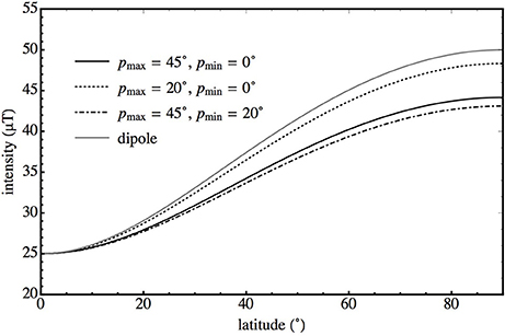
Figure 2. B^TAF (Equation4) calculated for four models as a function of latitude using a latitudinal bin size of 10°: 1) p_max = 45°, p_min = 0°, 2) p_max = 20°, p_min = 0° and 3) p_max = 45°, p_min = 20°. Additionally the standard dipole model (Equation1) is also calculated. In all four models the equatorial field was set to 25 μT, i.e., $B_{eq}^{TAF}=$ $B_{eq}^D$ = 25 μT.

All three models have a weaker latitudinal dependency than the dipole model of Equation (1) (Figure 2), that is, the effect of including dipolar secular variation into the TAF intensity model is to reduce the expected latitudinal dependence of the observed field, i.e., a TAF palaeointensity record cannot have the same latitudinal dependency as a GAD field. For a constant equatorial field the deviation between the dipole model and the TAF model is enhanced at high latitudes. This is expected: consider the case where the sampling locality is approximately at the geographic North Pole, i.e., s_max is slightly larger than s_min, but both are close to 0°, and p_min >> 0°, then the value of ${\overline{g}}_{s_{min}}^{s_{max}}$ used in Equation (4) is >0° reducing B^TAF at high latitudes; this effect is less pronounced for equatorial sampling localities. Generally the value of s_max was found to be more important than s_min, and the effect of bin size is relatively unimportant for bin sizes between 5° and 15°.

A Giant Gaussian Processes (GGP) Model Approach to Secular Variation

While the simple cap dipolar model demonstrates the effect of secular variation on binned palaeointensity data, it does not attempt to describe secular variation, as it is flat distribution. There is a class of models based on Giant Gaussian Processes (GGP) (Constable and Parker, 1988; Kono and Hiroi, 1996; Quidelleur and Courtillot, 1996; Constable and Johnson, 1999; Tauxe and Kent, 2004; Shcherbakov et al., 2014), that express secular variation by varying the Gauss coefficients $g_l^m,h_l^m$; the gauss coefficients have a mean and standard deviations (σ_l) that are a function of degree l. Generally the mean $g_1^0$ (axial dipole) and $g_2^0$ (axial quadrupole) are non-zero, and the higher order $g_m^0$ are zero, though occasionally non-zero mean $g_3^0$ (axial octupole) terms are considered (Tauxe and Kent, 2004) (Table 1).

TABLE 1

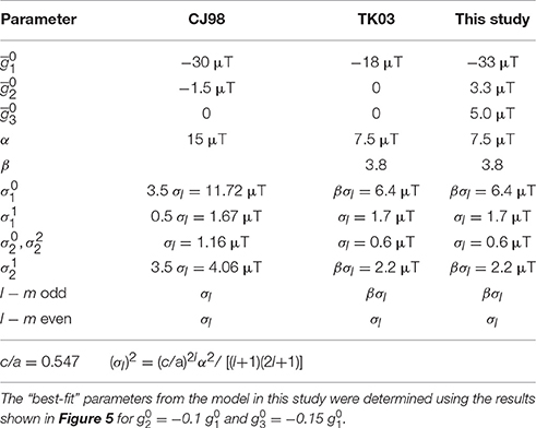
Table 1. Parameters for secular variation models considered in this paper. CJ98 is from Constable and Johnson (1999) and TK03 refers to Tauxe and Kent (2004).

The variation is partially accommodated by the α parameter, and is given by

$\begin{array}{cc}{\sigma }_l^2=\frac{{(c/a)}^{2l}{\alpha }^2}{(l+1)(2l+1)}& (5)\end{array}$

where c/a is the ratio of the core radius to that of the Earth's, and α a fitted parameter. Through time the models have developed, with increasing complexity used to describe the variation in the individual Gauss coefficients (Table 1). The early model of Constable and Parker (1988), did not accommodate the observed latitudinal variation in the scatter of the virtual geomagnetic pole (VGP) data. Later models did this by weighting some of the variance parameters (Quidelleur and Courtillot, 1996; Constable and Johnson, 1999; Tauxe and Kent, 2004) (Table 1).

Constable and Johnson (1999) compared their GGP model to the then palaeointensity record, and found a reasonable correlation. However, in the last 20 years the palaeointensity database has changed significantly, with the inclusion of far more high-latitude data points. Additionally, the selection criteria for drawing samples from the database are far more stringent now than it was in the late 1990s (e.g., Lawrence et al., 2009; Cromwell et al., 2015; Wang et al., 2015; Døssing et al., 2016). As we will see in the next section the GGP model of Constable and Johnson (1999) no longer explains the current PINT database.

Comparison of Current GGP Models with the Latitudinal Palaeointensity Data Record

To compare GGP models with the current palaeointensity data record, I selected Thellier data with pTRM checks from the PINT database (Biggin et al., 2009) from non-transitional (or unknown polarity) samples ≤5 Ma in age with at least three intensity estimates per unit, i.e., N ≥ 3, with a unit palaeointensity estimate standard deviation of <50%, as in previous studies (Døssing et al., 2016). This yields 496 field estimates. I also combined the northern and southern hemisphere data, because the southern hemisphere data is very limited both spatially and temporally for the last 5 Myr. For example, for a 10° bin size, several of the southern hemisphere bins have no data, and others have only one dataset covering narrow time periods, e.g., data from Tristan da Cunha (Shah et al., 2016) is the single data set in the −30 to −40° bin and covers a time period of <50 kyr. After folding and binning at 10° steps, the 80–90° bin has no data, but the next least populated bin, the 0–10° bin, has eight points.

To determine a value for each bin, Døssing et al. (2016) calculated the median of the data in each bin. Whilst this approach makes less assumptions, if we compare the bin with the most data points (bin 10–20°, 226 points,), we see that at 95% confidence it can be described as Gaussian (Figure 3). I therefore calculate the mean for each bin, rather than the median (Figures 4, 5). I also determine a 95% confidence limit for each bin. The limits are effected by the number of points in each bin; the 10–20° bin has the narrowest confidence interval (Figure 4). The mean data are seen to increase with latitude until the 50–60° bin, then decrease; however, the site data are very scattered (Figure 3). The simple dipole model Equation (1) increases more rapidly than the data (Figure 4), and does not describe the data. Nor do the simple cap models (Figure 2) describe the data trend (Figure 4).

FIGURE 3

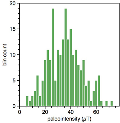
Figure 3. Histogram of bin count vs. intensity for the palaeointensity data from the PINT palaeointensity database (Biggin et al., 2009, http://earth.liv.ac.uk/pint), for the 10–20° bin. The palaeointensity data were selected from the PINT database from sites ≤5 Ma, for which there were at least three intensity estimates. The northern and southern hemisphere data are combined. The data is not distinguishable from a Gaussian distribution at 95% confidence.

FIGURE 4

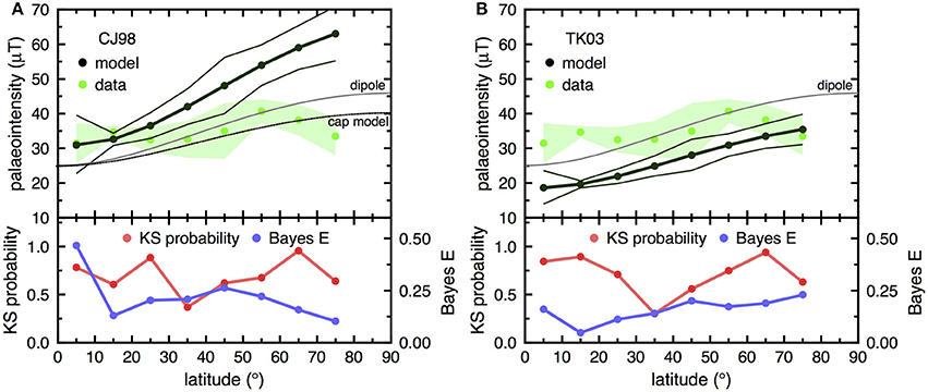
Figure 4. GGP model intensity predictions vs. latitude for: (A) CJ98 model, and (B) TK03 model. Also depicted are palaeointensity data (green dots) from the PINT palaeointensity database (Biggin et al., 2009, http://earth.liv.ac.uk/pint), which has been binned at 10° degree intervals and the mean determined. The palaeointensity data were selected from the PINT database from sites ≤5 Ma, for which there were at least three intensity estimates. The northern and southern hemisphere data are combined; there is no data >80°. 95% confidence intervals are plotted for the PINT data (shaded green) and the model data (black lines). Additionally the standard dipole model (Equation1) is also calculated, with $B_{eq}^D$ = 25 μT (gray line), in (A) a cap model as shown in Figure 3 (p_max = 45°, p_min = 20°). In the lower section of the figures the Kolmogorov-Smirnov probability and the Bayes error E are plotted as a function of latitude.

FIGURE 5

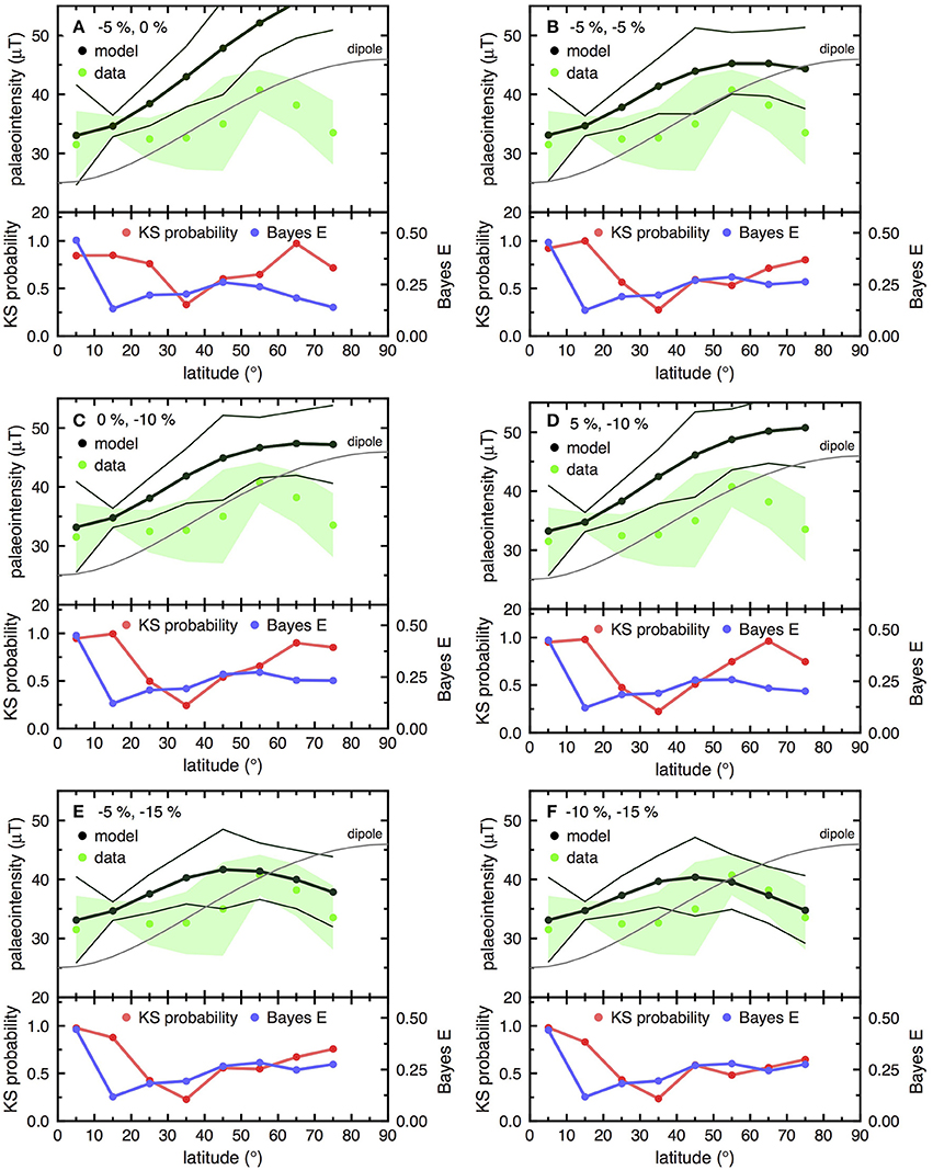
Figure 5. GGP model intensity predictions vs. latitude for: (A) $g_2^0$ ≈ −0.05 $g_1^0$ (−5%) and $g_3^0$ ≈ 0 (0%), (B) $g_2^0$ ≈ −0.05 $g_1^0$ and $g_3^0$ ≈ −0.05 $g_1^0$, (C) $g_2^0$ ≈ 0 and $g_3^0$ ≈−0.1 $g_1^0$, (D) $g_2^0$ ≈ 0.05 $g_1^0$ and $g_3^0$ ≈ −0.1 $g_1^0$, (E) $g_2^0$ ≈ −0.05 $g_1^0$ and $g_3^0$ ≈ −0.15, and (F) $g_2^0$ ≈ −0.1 $g_1^0$ and $g_3^0$ ≈ −0.15 $g_1^0$. Included are the binned palaeointensity data (green dots) from the PINT palaeointensity database. The northern and southern hemisphere data are combined; there is no data >80°, 95% confidence intervals are plotted for the PINT data (shaded green) and the model data (black lines). Additionally, the standard dipole model (Equation1) is also calculated, with $B_{eq}^D$ = 25 μT (gray line). In the lower section of the figures the Kolmogorov-Smirnov probability and the Bayes error E are plotted as a function of latitude.

I next compare the CJ98 and TK03 GGP models (Table 1) with the selected PINT data, and determine 95% confidence intervals using the number of PINT data in each bin to calculate the models' confidence limits for comparison with the data (Figure 4). It is visually clear that neither of these two models follows the binned palaeointensity latitudinal trend. CJ98 and TK03 both increase too rapidly with latitude, plus TK03 is too low at the equator. Adjusting the $g_1^0$ term for TK03 model does not resolve the latitudinal variation inconsistency. To statistically estimate if the model and PINT data distributions are distinct, I calculated two parameters: (1) the Kolmogorov-Smirnov (KS) distribution probability (Press et al., 2007), and (2) the Bayes error (Braga Neto and Dougherty, 2015). The KS distribution probability estimates the likelihood that the data distributions for each bin are drawn from the same distribution, i.e., low probability values suggest that the distributions are significantly different (Press et al., 2007). The KS distribution probability examines only the shape of the distributions at each bin, but is invariant to absolute values. To quantify the absolute overlap between two normal distributions, I calculate the upper bound on the Bayes error (Braga Neto and Dougherty, 2015), to estimate the maximum misclassification error between two normal distributions with means μ₀ and μ₁ and standard deviations σ₀ and σ₁. This is done by finding the value of γ, where 0 < γ < 1, which minimizes c_γ.

$\begin{array}{cc}{c}_{\gamma }=\underset{\alpha \epsilon (0,1)}{\text{min}}\left[\frac{{\sigma }_0^{1-\gamma }{\sigma }_1^{\gamma }}{\sqrt{(1-\gamma ){\sigma }_0^2+\gamma {\sigma }_1^2}}\exp \left(\frac{(\gamma -1)\gamma {({\mu }_0-{\mu }_1)}^2}{2(\gamma {\sigma }_1^2-(\gamma -1){\sigma }_0^2)}\right)\right]& (6)\end{array}$

If we assume a priori that the probabilities that the observation came from each of the distributions is equal, then the upper bound on the probability of a misclassification error is E ≤ c_γ/2. If E = 0, there is no probability of a misclassification, i.e., the two distributions are completely distinct from each other, and if E = 0.5 there is a 50:50 chance that misclassification will take place, therefore the two distributions must be identical. However, the probabilistic nature of the analysis can just be taken as an intuitive measure of the similarity between two distributions.

For CJ98 and TK03, both the KS distribution probability and the Bayes E are generally low, indicating that the models do not accurately describe the data. For CJ98, Bayes E is >0.45 for the 0–10° bin, this is partially an artifact of the two mean values being similar.

Permanent Non-Dipole Features and the Palaeointensity Data Record

It is clear both by inspection and the statistical tests that the CJ98 and TK03 models to not accommodate the paleointensity data (Figure 4). To explore this mismatch, I examined the GGP models, starting with the TK03 model of Tauxe and Kent (2004). There are many parameters (Table 1) that can potentially change the shape of the geomagnetic field (Constable and Johnson, 1999; Merrill and McFadden, 2003), however, whilst changes to the standard deviation parameters can drastically increase the secular variation, when averaged over long periods of time, variations in these parameters contribute more to the scatter rather than the mean trend, which still resembles a dipole field, albeit reduced, as demonstrated in the simple cap model (Figure 2).

To change the model trends to resemble something closer to the PINT database, it is necessary to add permanent non-dipole terms, in particular $g_2^0$ (axial quadrupole) and $g_3^0$ (axial octupole). In TK03 (Table 1) $g_2^0$ is set to zero, however, in most other GGP models (Constable and Parker, 1988; Quidelleur and Courtillot, 1996; Constable and Johnson, 1999; Tauxe, 2005; Shcherbakov et al., 2014), this term is non-zero and of the same sign as $g_1^0$. The literature provides some indications of what values of $g_2^0$ and $g_3^0$ are considered “reasonable”: Using palaeomagnetic data for the last 5 Myrs, various studies have inverted the palaeomagnetic data to determine the time-averaged Gauss coefficients (e.g., Johnson and Constable, 1997; Carlut and Courtillot, 1998; Kono et al., 2000; Johnson et al., 2008). Of these studies, only that of Kono et al. (2000) attempted to fully invert the palaeointensity data record. They found that $g_2^0$ ≈ −0.06 $g_1^0$ and $g_3^0$ ≈ 0.06 $g_1^0$, which is in contrast to the palaeodirectional data only inversions that generally predict that $g_2^0$ and $g_3^0$ have the same sign as $g_1^0$; the exception being some of the inversions for single polarities (Johnson and Constable, 1997; Johnson et al., 2008), where $g_3^0$ was found to be of opposite sign to $g_1^0$. Using geodynamo simulations, Veikkolainen et al. (2017) examined the entire PINT database, in an attempt to quantify the contribution of $g_2^0$ and $g_3^0$ to the TAF through examination of palaeointensity frequency distribution. They found that the paleointensity record is best described by periods of different $g_1^0$ intensities, however, each period had a ±10% octupole field contribution, with a minimal quadrupole contribution.

Given the limited number of binned data (8 points), the aim of the exploration was to reproduce the same trends as observed in the data and not to determine an exact fit. Therefore, in the following calculations, I varied only the $g_1^0$, $g_2^0$, and $g_3^0$ terms within the TK03 model. I normalized the TK03 model with respect to the most accurate PINT database bin (10–20° bin), i.e., $g_1^0$was calculated for each model. This normalizing clearly affects the Bayes error, however, it is consistent across the models for comparison.

Adding $g_2^0$ and $g_3^0$ terms of the same sign as $g_1^0$ simply increases the latitudinal variation, and makes the fit between the models and the data worse than when $g_2^0$ and $g_3^0$ are both zero. Therefore, to match the PINT database trends for the last 5 Myrs, permanent $g_2^0$ and $g_3^0$ terms of the opposite sign to $g_1^0$ are required. Various combinations of $g_2^0$ and $g_3^0$ are plotted in Figure 5; $g_2^0$ and $g_3^0$ are expressed as percentages of $g_1^0$. The effect of introducing $g_2^0$ and $g_3^0$ of the opposite sign to $g_1^0$ is to decrease the rate of latitudinal increase, producing a ‘flatter’ trend. It was found that to represent the data trend at high latitudes under the constraint $g_2^0$, $g_3^0$ < 0.2 $g_1^0$, both $g_2^0$ and $g_3^0$ have to be of the opposite sign to $g_1^0$.

In Figure 5A, I consider a 5% quadrupole field with no octupole field, as suggested by several palaeodirectional studies (e.g., Carlut and Courtillot, 1998). I plot only the case where $g_2^0$ = −0.05 $g_1^0$, as this trend matches the data better than for $g_2^0$ = +0.05 $g_1^0$, however, its latitudinal dependency is too high even for the negative contribution. Adding a $g_2^0$ = +0.05 $g_1^0$ term to this figure, i.e., approximately the same configuration as suggested by Kono et al. (2000), makes the mismatch between model and data worse than in Figure 5A. The effect of adding a $g_3^0$ = −0.05 $g_1^0$ term to a $g_2^0$ = −0.05 $g_1^0$, sharply decreases the field intensity at high-latitudes (Figure 5B). The behavior for mixed quadrupole/octupole −5% contribution (Figure 5B) is similar to that of a pure octupole term of −0.1 $g_1^0$ (Figure 5C). This latter configuration is the same as that suggested Veikkolainen et al. (2017) who examined the entire PINT database. Attempting to combine quadrupole and octupole terms of opposite signs does not improve the data fit (Figure 5D). The models that best describe the data are shown in Figures 5E,F; that is, $g_3^0$ = −0.15 $g_1^0$ and $g_2^0$ = −0.05 and −0.1 $g_1^0$. Even within these models there is still a large degree of mismatch at mid-latitude. The $g_1^0$ term determined by fitting the models to the 10–20° bin, was consistently between 33.0 and 33.2 μT, a little larger than the values commonly quoted, e.g., 30 μT (Constable and Johnson, 1999; Shcherbakov et al., 2014).

The $g_2^0$ and $g_3^0$ contributions are higher than that found from the directional palaeomagnetic data (e.g., Carlut and Courtillot, 1998), however, this is not inconsistent. The large $g_3^0$ was needed to accommodate the high-latitude palaeointensity data behavior; it is well-documented that palaeointensity data is more sensitive to high-latitude geomagnetic field behavior than declination and inclination data (Constable, 2007). Therefore, it appears that the paleointensity database is highlighting high-latitudinal behavior not accessible to the declination and inclination data. Veikkolainen et al. (2017) who also studied only the palaeointensity record, also concluded that large permanent octupole features are required to explain database trends. In contrast to this study, Kono et al. (2000) found $g_2^0$ ≈ −0.06$g_1^0$ and $g_3^0$ ≈ 0.06$g_1^0$ for the TAF (0–5 Ma), i.e., $g_3^0$ is of the same sign as $g_1^0$; however, as stated above the palaeointensity database has improved significantly since the late 1990s.

The KS probability was consistently low for bin 30–40°; with 65 points it was the second most populated bin, and is normal at 95% confidence (Figure 5). That is, the GGP distribution prediction for this bin does not follow the observed behavior well-regardless of $g_2^0$ and $g_3^0$ contributions. Given the problematic nature of palaeointensity collection, it is suggested more data at this mid-latitude are required.

Conclusions

This paper has shown through a simple cap model of secular variation that a TAF intensity field cannot theoretically display the same behavior as a pure GAD, and will always have a trend that is less dependent on latitude (Figure 2). However, the simple cap model does not explain the latitudinal behavior seen in the PINT database (Figure 4). Through the use of GGP models it was found that the TAF (0–5 Ma) has likely permanent non-dipole features, in particular an axial quadrupole term ≈ −0.1$g_1^0$ and octupole term ≈ −0.15$g_1^0$. The $g_1^0$ term was determined to be ~33 μT. These permanent non-dipole features are larger than reported in other studies, however, these other studies either examined only the directional palaeomagnetic data (e.g., Carlut and Courtillot, 1998) or considered much early versions of the palaeointensity database where the high-latitude palaeointensity data is less constrained than today (Constable and Johnson, 1999). However, while the PINT database has far more data now than 20 years ago, the data at high-latitudes, even after folding, are very limited and subject to incomplete temporal sampling; more high-latitude data are required. Data within the 30–40° bin also displays unusual behavior, which would benefit from more data.

Author Contributions

The author confirms being the sole contributor of this work and approved it for publication.

Conflict of Interest Statement

The author declares that the research was conducted in the absence of any commercial or financial relationships that could be construed as a potential conflict of interest.

Acknowledgments

AM would like to thank Dr. David Heslop for fruitful discussions regarding Bayes error analysis.

References

Biggin, A. J., Strik, G. H. M. A., and Langereis, C. G. (2009). The intensity of the geomagnetic field in the late-Archaean: new measurements and an analysis of the updated IAGA palaeointensity database. Earth Planets Space 61, 9–22. doi: 10.1186/BF03352881

CrossRef Full Text | Google Scholar

Braga-Neto, U. M., and Dougherty, E. R. (eds.). (2015). “Performance analysis,” in Error Estimation for Pattern Recognition (Hoboken, NJ: John Wiley & Sons, Inc.). doi: 10.1002/9781119079507.ch3

CrossRef Full Text

Carlut, J., and Courtillot, V. (1998). How complex is the time-averaged geomagnetic field over the past 5 Myr? Geophys. J. Int. 134, 527–544.

Google Scholar

Constable, C. (2007). “Centeniial- to Milennial-Scale Geomagnetic Field Variations,” in Treatise on Geophysics, Vol. 5, Geomagnetism, ed M. Kono (Amsterdam: Elsevier), 337–372.

Constable, C. G., and Johnson, C. L. (1999). Anisotropic paleosecular variation models: implications for geomagnetic field observables, Phys. Earth Planet. Inter. 115, 35–51. doi: 10.1016/S0031-9201(99)00065-5

CrossRef Full Text | Google Scholar

Constable, C. G., and Parker, R. L. (1988). Statistics of the geomagnetic secular variation for the past 5 My. J. Geophys. Res. 93, 11569–11581. doi: 10.1029/JB093iB10p11569

CrossRef Full Text | Google Scholar

Cromwell, G., Tauxe, L., and Halldórsson, S. A. (2015). New paleointensity results from rapidly cooled Icelandic lavas: implications for Arctic geomagnetic field strength. J. Geophys. Res. 120, 2913–2934. doi: 10.1002/2014JB011828

CrossRef Full Text | Google Scholar

Døssing, A., Muxworthy, A. R., Supakulopas, R., Riishuus, M. S., and Mac Niocaill, C. (2016). High northern geomagnetic field behavior and new constraints on the Gilsa event: paleomagnetic and Ar-40/Ar-39 results of similar to 0.5-3.1 Ma basalts from Jokuldalur, Iceland, Earth Planet. Sci. Lett. 456, 98–111. doi: 10.1016/j.epsl.2016.09.022

CrossRef Full Text

Jackson, A., Jonkers, A. R. T., and Walker, M. R. (2000). Four centuries of geomagnetic secular variation from historical records. Philos. Trans. R. Soc. A 358, 957–990. doi: 10.1098/rsta.2000.0569

CrossRef Full Text | Google Scholar

Johnson, C. L., and Constable, C. G. (1997). The time-averaged geomagnetic field: global and regional biases for 0-5 Ma. Geophys. J. Int. 131, 643–666. doi: 10.1111/j.1365-246X.1997.tb06604.x

CrossRef Full Text | Google Scholar

Johnson, C. L., Constable, C. G., Tauxe, L., Barendregt, R., Brown, L. L., Coe, R. S., et al. (2008). Recent investigations of the 0-5 Ma geomagnetic field recorded by lava flows. Geochem. Geophys. Geosyst. 9:Q04032. doi: 10.1029/2007GC001696

CrossRef Full Text | Google Scholar

Kono, M., and Hiroi, O. (1996). Paleosecular variation of field intensities and dipole moments. Earth Planet. Sci Lett. 139, 251–262.

Google Scholar

Kono, M., Tanaka, H., and Tsunakawa, H. (2000). Spherical harmonic analysis of paleomagnetic data: the case of linear mapping. J. Geophys. Res. 105, 5817–5833. doi: 10.1029/1999JB900050

CrossRef Full Text | Google Scholar

Lawrence, K. P., Tauxe, L., Staudigel, H., Constable, C. G., Koppers, A., McIntosh, W., et al. (2009) Paleomagnetic field properties at high southern latitude. Geochem. Geophys. Geosyst. 10:Q01005. doi: 10.1029/2008GC002072

CrossRef Full Text | Google Scholar

Merrill, R. T., and McFadden, P. L. (2003). The geomagnetic axial dipole field assumption. Phys. Earth Planet. Inter. 139, 171–185. doi: 10.1016/j.pepi.2003.07.016

CrossRef Full Text | Google Scholar

Press, W. H., Flannery, B. P., Teukolsky, S. A., and Vetterling, W. T. (2007). Numerical Recipes: The Art of Scientific Computing. New York, NY: Cambridge University Press.

Google Scholar

Quidelleur, X., and Courtillot, V. (1996). On low-degree spherical harmonic models of paleosecular variation. Phys. Earth Planet. Inter. 95, 55–78. doi: 10.1016/0031-9201(95)03115-4

CrossRef Full Text | Google Scholar

Shah, J., Koppers, A. A. P., Leitner, M., Leonhardt, R., Muxworthy, A. R., Heunemann, C., et al. (2016). Palaeomagnetic evidence for the persistence or geomagnetic main field anomalies in the South Atlantic. Earth Planet. Sci. Lett. 441, 113–124. doi: 10.1016/j.epsl.2016.02.039

CrossRef Full Text | Google Scholar

Shcherbakov, V. P., Khokhlov, A. V., and Sycheva, N. K. (2014). Comparison of the Brunhes epoch geomagnetic secular variation recorded in the volcanic and sedimentary rocks. Izvest. Phys. Solid Earth 50, 222–228. doi: 10.1134/S1069351314020098

CrossRef Full Text | Google Scholar

Tauxe, L. (2005). Inclination flattening and the geocentric axial dipole hypothesis. Earth Planet. Sci. Lett. 233, 247–261. doi: 10.1016/j.epsl.2005.01.027

CrossRef Full Text | Google Scholar

Tauxe, L. (2010). Essentials of Paleomagnetism. Berkley, CA: University of California Press.

Google Scholar

Tauxe, L., and Kent, D. V. (2004). “A simplified statistical model for the geomagnetic field and the detection of shallow bias in paleomagnetic inclinations: Was the ancient magnetic field dipolar?” in Timescales of the Paleomagnetic Field, eds J. E. T. Channell, D. V. Kent, W. Lowrie, and J. G. Meert (Washington, DC: AGU), 101–115.

Google Scholar

Valet, J. P. (2003). Time variations in geomagnetic intensity. Rev. Geophys. 41:1004. doi: 10.1029/2001RG000104

CrossRef Full Text | Google Scholar

Veikkolainen, T., Heimpel, M., Evans, M. E., Pesonen, L. J., and Korhonen, K. (2017). A paleointensity test of the geocentric axial dipole (GAD) hypothesis. Phys. Earth Planet. Inter. 265, 54–61. doi: 10.1016/j.pepi.2017.02.008

CrossRef Full Text | Google Scholar

Wang, H., Kent, D. V., and Rochette, P. (2015). Weaker axially dipolar time-averaged paleomagnetic field based on multidomain-corrected paleointensities from Galapagos lavas. Proc. Natl. Acad. Sci. U.S.A. 112, 15036–15041. doi: 10.1073/pnas.1505450112

PubMed Abstract | CrossRef Full Text | Google Scholar

Wilson, R. L. (1970). Permanent aspects of the earth's non-dipole magnetic field over upper tertiary times. Geophys. J. R. Astron. Soc. 19, 417–437. doi: 10.1111/j.1365-246X.1970.tb06056.x

CrossRef Full Text | Google Scholar