Petrological Geodynamics of Mantle Melting I. AlphaMELTS + Multiphase Flow: Dynamic Equilibrium Melting, Method and Results

Introduction

Melting in the Earth's interior is a complex process that involves rocks which are essentially multiphase and multicomponent chemical systems. The process is usually non-stationary in the sense that the solid and the melt products are dynamical systems. These systems may also experience different levels of chemical equilibration and the associated thermal state can be transient.

Traditionally from a petrological point of view melting is described by a system in which the solid and local melt product are in complete chemical equilibrium. As the temperature or pressure or a combination of both varies, the sum of the melt products either remains constantly in chemical equilibrium with the local residual solid (batch melting) or the whole melt is assumed to be chemically isolated from the local solid (fractional melting). In these models the spatial and temporal settings are usually not significant. The chemical evolution of igneous rocks has been quantified by parameterized compositional models based mainly on petrological experimental studies (e.g., Langmuir et al., 1992; Herzberg et al., 2007; Herzberg and Asimow, 2008). More comprehensive models have been also presented (Spera and Bohrson, 2001). The chemical thermodynamic approach developed over several years by Ghiorso (Ghiorso, 1985; Ghiorso and Sacks, 1995; Ghiorso et al., 2002) specifically includes the melt phase and provides a more rigorous understanding of the petrological evolution at different P,T,X,fO₂ conditions. Recently new thermodynamic descriptions of mantle melting have been presented (Ueki and Iwamori, 2014; Jennings and Holland, 2015). An advantage of the thermodynamic formulation is that, within certain limits, it creates a framework that allows also to make predictions at conditions not interested by experimental studies. The petrological evolution over time and space remains still undefined or it can only be inferred qualitatively. This is a recurrent shortcoming of qualitative and quantitative inverse studies that rely only on petrological and geochemical evidences from field observations and a simplified description of the process involved. Few studies (Asimow and Stolper, 1999; Asimow, 2002) made a serious attempt to interface transport principles with the thermodynamic melt approach. The experience from these studies has been somehow translated in the program AlphaMELTS (Smith and Asimow, 2005) which is a powerful interface of Ghiorso's thermodynamic model with additional features, such as melt focusing, melting along an adiabatic thermal gradient and modeling of trace elements.

The dynamic nature of melting has been investigated for some time using two-phase flow models (McKenzie, 1984; Scott and Stevenson, 1984, 1986; Spiegelman, 1993a; Richardson, 1998; Ghods and Arkani-Hamed, 2000; Schmeling, 2000; Bercovici et al., 2001; Bercovici and Ricard, 2003; Šrámek et al., 2007; Hewitt and Fowler, 2008; Katz, 2008; Hewitt, 2010; Rudge et al., 2011) all derived from a more general analysis of the two-phase flow process (Ishii and Hibiki, 2006). The scope was mainly to understand the physical behavior of melt from an ideal standpoint. Usually the characterization of the melt products has been associated to ideal or simplified chemical systems not necessarily related to any specific crustal or mantle rock.

The idea of combining a more realistic petrological description of melt with a transport model is conceptually very simple although the actual implementation is not quite straightforward. For instance the thermodynamic formulation developed by Ghiorso cannot be easily combined with a numerical transport model. Beside an early attempt using a parameterized petrological formulation (Cordery and Morgan, 1993), the few studies that overcome these difficulties (Katz, 2008; Tirone et al., 2009, 2012) applied simplified thermodynamic formulations. The obvious shortcoming is that the petrological results of these models may not be sufficiently accurate to interpret real petrological field data. In addition, because thermodynamic equilibrium principles are applied, chemical equilibrium needs to be necessarily imposed at some spatial and temporal scale. It remains to be seen whether this is the correct approach to describe the melting process in the Earth's interior. A different approach that would consider a kinetic formulation perhaps in combination with a thermodynamic model could be a valid alternative. However such general formulation for a multi-mineral system (mantle rock assemblage+melt) described by several chemical components is not quite available yet. A first attempt using a simplified kinetic model for binary systems has been applied to dynamic disequilibrium melting (Rudge et al., 2011). One major difficulty is that experimental data to constrain any possible kinetic model are scarce. A possible solution that could make this type of modeling more tractable would require to impose thermodynamic equilibrium on a certain spatial and temporal scale determined by (existing and future) kinetic experimental data. An example of interfacing thermodynamics and kinetics, but for a much more limited purpose, can be found in a recent study (Tirone et al., 2016b), where the program AlphaMELTS (Smith and Asimow, 2005) was used to constrain the compositional growth of olivine phenocrystals during a cooling process. The phenocrystals were considered chemically isolated from the melt although not physically removed from it, and at the same time chemical diffusion was allowed to develop within individual crystals.

One of the objectives of this study is to understand how the composition and distribution of melt and solid are affected by the dynamic evolution of the system assuming a 1-D mantle column. To go beyond a theoretical or ideal case study and to open up the possibility of interpreting real field geochemical and petrological observations, AlphaMELTS (Smith and Asimow, 2005) and the included thermodynamic model have been chosen as the petrological tool that is coupled with the dynamic model. The aim is also to present the dynamic formulation in a simple and practical form that describes with reasonable accuracy (a) the transport of a solid dynamic phase (mantle), and one or two fluid phases (specifically melt and water-based fluid), (b) the evolution of the composition of each dynamic phase and (c) the thermal state over time and space. While the simultaneous numerical solution of several coupled differential equations may seem a formidable task, the motivation for this study is also to illustrate how a numerical procedure applied to the equations describing the transport model can be accomplished without a very advanced knowledge of numerical methods. In this first of a series of three studies the local thermodynamic equilibrium between solid and melt is assumed on the spatial scale defined by the numerical grid on a certain time interval in a 1-D mantle column (Figure 1). Certain parameters discussed in the following sections are varied to investigate the effect on the melt production and chemical evolution over time and space. The second contribution of this series will consider an alternative scenario, that is the case in which, once the melt is formed, it does not interact chemically any further with the residual solid while still affecting the dynamic model. The melt products converge into a different system that still evolves according to equilibrium principles but separately from the residual solid. This can be accomplished by applying the thermodynamic formulation to two local sub-systems separately. In the third and last contribution of the series the effect of water on the melting process is investigated by combining chemical thermodynamics with a three-phase flow model.

FIGURE 1

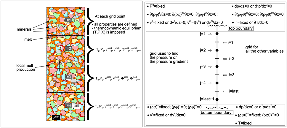
Figure 1. (Left) Schematic view of the mantle column. In the dynamic equilibrium melting (DEM) model at each grid point local equilibrium is assumed between melt and solid. Dynamic and thermodynamic properties represent the average spatial values within each grid point. The drawing describes only the concept of the model, distribution of melt and minerals in the figure not in scale. (Right) Illustration of the two spatial grids, the j-grid used for the pressure or the pressure gradient, and the i-grid for all the other variables. Boundary conditions at the top and bottom of the model are also reported. The zero gradient condition, for example ∂(ρϕ)/∂z = 0, means that (ρϕ)_{top boundary} = (ρϕ)_{i = 1} or (ρϕ)_{bottom boundary} = (ρϕ)_{i = last}.

Perhaps at this point it is worth summarizing the different models that will be described. The general definition of dynamic equilibrium melting (DEM) is not entirely accurate but it captures the essence of a combination of a transport model and a thermodynamic approach. The more correct definition, something like “1-system 2 (or 3)-phase flow thermo mechanical and chemical equilibrium melting model” is clearly impractical. Similarly a dynamic batch melting model that is defined when the velocity of the solid and melt are assumed to be equal is also quite intuitive although not necessarily rigorous. These two type of models can be considered an extension of concepts developed in a previous study (Asimow and Stolper, 1999). For the dynamic batch melting model (υ^s = υ^m), chemical exchange between the solid and melt is associated to the mass transfer between these two components but also to chemical re-equilibration, for example Fe-Mg redistribution, as the external conditions, such as P and T, are allowed to vary. It should be clear that everything is confined within the local system (i.e., spatial grid point), in other words the system solid+melt is closed to external mass transfer and the local bulk composition is fixed. When the dynamics of the solid assemblage and melt phase are different (υ^s ≠ υ^m), the principles dictating the chemical evolution remain the same but the local system solid+melt is open to mass transfer from outside (i.e., nearby spatial grid points), hence the relative abundance is not only controlled by the local melting process and the bulk composition of the system may vary.

To complete the model definitions in the second contribution of the series a dynamic fractional melting (DFM) model will be introduced to describe a dynamic melting process in which the chemical equilibrium approach applies to two separate sub-systems, one for the residual solid and one for the sum of the melt products. The last model that considers dynamic fractional melting when the velocity of the solid and melt are assumed to be equal is simply named dynamic fractional melting with υ^s = υ^m. This idealization of the fractional melting concept is not new since it was first introduced in an earlier study (Asimow, 2002).

Description of the Multiphase Dynamic Model

The relevant transport equations for a 1-D multiphase dynamic model are introduced in this section. While none of the material is entirely new, it may be useful to review the essential features of the formulation. In the Eulerian description the properties are determined at fixed points in space where each point represents a small control volume. Since multiple assemblages (solid rock, melt, water) are considered simultaneously and their dynamic evolution is treated separately, the distribution of each of these assemblages or dynamic phases can be described by a different differential equation for the conservation of mass (Ishii and Hibiki, 2006):

$\begin{array}{ll}\frac{\partial \left({\rho }^a{\varphi }^a\right)}{\partial t}+\frac{\partial \left({\upsilon }^a{\rho }^a{\varphi }^a\right)}{\partial z}={\Gamma }^a\hfill & (1)\hfill \end{array}$

where the superscript a stands for the dynamic phase or assemblage “s⇒solid,” “m⇒melt,” or “w⇒water.” ρ is the mass density of the dynamic phase, ϕ^a is the fraction of the control volume occupied by the dynamic phase a and υ is the velocity of the dynamic phase. The product ρϕ, later labeled Φ, can be seen as the mass of a certain dynamic phase per unit volume that is associated to the fraction ϕ of the control volume occupied by the dynamic phase. For instance, if ρ is 3,000 kg/m³, ϕ is 0.3 and the control volume is 2 m³ then the total mass of the dynamic phase in the fraction ϕ of the total volume would be 3,000 × 0.3 × 2. Each assemblage is allowed to exchange mass, for example when at a particular point in space melting of the solid takes place, the total mass of the solid should decrease and the total amount of melt should correspondingly increase. This process is accounted for by the term Γ^a which is the cumulative mass transfer rate that includes the exchange between the transport phase a with the other transport phases (e.g., for solid a = s then Γ^s = Γ^s−m + Γ^{s − w}). Mass transfer to a certain dynamic phase (e.g., from m to s) has a counterpart (from s to m) and the two quantities are related, Γ^s−m = −Γ^m−s.

The equation of motion for the solid assemblage is described in a 1-D problem by the following relation:

$\begin{array}{ll}-{\varphi }^s\frac{\partial P}{\partial z}+{\varphi }^s{\rho }^{s}g-M^{s-m}-M^{s-w}+S=0\hfill & (2)\hfill \end{array}$

where the acceleration terms have been ignored (∂(ρ^sϕ^sυ^s)/∂t + ∂(ρ^sϕ^sυ^s2)/∂z ≈ 0) (Bird et al., 2002). The first and last term in Equation (2) describe the change by pressure (P) and viscous forces (S), the second term describes the effect of gravitational forces and the M terms are similar to the mass transfer rate introduced in the mass conservation equations and they describe the dynamic coupling of motion of the assemblages. Unlike the mass transfer rate, M can assume different forms, depending on the nature of the dynamic systems and the type of interaction among them. The presence of a third dynamic phase (water) will be considered in the third and last contribution of the series, however the relevant relations are introduced here since the formulation of the two-phase flow model, specifically addressed in this study, can be derived by simply assuming that no water is present in the system (ϕ^w = 0). The motion coupling between the solid and melt assemblages is described by the following relation M^s−m = −(ϕ^m2μ^m/k^m)(υ^m − υ^s) where μ^m is the viscosity of melt. The permeability is defined as k^m = ϕ^m3Ω^m4/C where Ω^m = ϕ^m/(ϕ^m + ϕ^w) and C is a permeability constant. When water is ignored the above equation for the permeability k^m is similar to the relation used in several studies on melt porous flow (e.g., McKenzie, 1984; Spiegelman, 1993a; Schmeling, 2000; Rudge et al., 2011). An expression similar to M^s−m can be used for the interaction between solid and water M^{s − w}, while no interaction is assumed between melt and water. The permeability for water assumes a slightly different form, k^w = ϕ^w3Ω^w2(1 − Ω^m2)/C where Ω^w = ϕ^w/(ϕ^m + ϕ^w). The relations just outlined here describe a simplified formulation borrowed from reservoir modeling which typically involves several phases like oil, gas and water (Corey et al., 1956; Stone, 1970; Peaceman, 1977; Dria et al., 1993; Abreu et al., 2006).

In two-phase flow problems alternative physical interpretations of the pressure and viscous forces S have been proposed in the past. In the earliest the pressure has been referred to the whole system and the generalized Newton's law of viscosity includes a bulk (or dilatational) viscosity term (McKenzie, 1984). A different formulation considered distinct pressures in the fluid and solid and an explicit definition of the bulk viscosity (Scott and Stevenson, 1986; Bercovici et al., 2001; Bercovici and Ricard, 2003; Simpson et al., 2010). The two can be reconciled under certain assumptions. A discussion on this point can be found elsewhere (Bercovici and Ricard, 2003; Rudge et al., 2011), It is only mentioned here that the pressure P would need to assume the meaning of an interfacial pressure between the fluid and the solid (Rudge et al., 2011). The standard definition of the pressure acting on the system would apply instead when the fluid is completely removed.

The expression for the variation of the viscous forces in a 1-D Cartesian geometry assumes the following form: $S=-\partial {\varphi }^s{\tau }_{zz}/\partial z$ where τ_zz is the vertical stress component. When no formal distinction is made between shear viscosity and bulk viscosity, the generalization of the Newton's law of viscosity (Bird et al., 2002) for the stress component τ_zz is ${\tau }_{zz}=-(7/3)\mu \partial {\upsilon }^s/\partial z$. Considering for simplicity the following relation μ^s = (7/3)μ where μ^s is assumed to represent the viscosity of the solid in the system, then the viscous Newtonian forces S can be described for a 1-D problem by the following simplified equation S = ∂ϕ^sμ^s∂υ^s/∂z². McKenzie (1984) suggested that μ^s could be related to the viscosity of the solid in absence of any fluid ${\mu }_0^s$ (i.e., ${\mu }^s={\mu }_0^s$). An alternative formulation that includes a dependence on the volume of the fluid has been also proposed (Scott and Stevenson, 1984, 1986; Bercovici et al., 2001; Bercovici and Ricard, 2003). In this study the dependence on melt is expressed by the following relation ${\mu }^s={\mu }_0^s(1+1/{\varphi }^m)$ which includes a term representing the relation between the bulk viscosity and the melt volume fraction. Similar but more complex expressions have been used in previous studies (Schmeling, 2000; Rudge et al., 2011). The essential feature of this expression for the viscosity is that the second term becomes dominant when the fluid or melt abundance is small. For practical purposes, below a certain threshold value for ϕ^m, the above equation is replaced by ${\mu }^s={\mu }_0^s$. Both definitions of μ^s have been considered in this study, and a discussion on the results using the two viscosity models will be presented in a later section.

The equation of motion for melt is similar to the one for the solid phase but with few differences. The interaction between melt and water (M^m−w) and the term related to the viscous forces are ignored, hence:

$\begin{array}{ll}-{\varphi }^m\frac{\partial P}{\partial z}+{\varphi }^m{\rho }^{m}g+M^{s-m}=0\hfill & (3)\hfill \end{array}$

The above equation for melt, and the similar equation for water, can be rearranged to express υ^m (and υ^w) explicitly:

$\begin{array}{ll}{\upsilon }^m=-\frac{k^m}{{\varphi }^m{\mu }^m}\left(\frac{\partial P}{\partial z}-{\rho }^{m}g\right)+{\upsilon }^s\hfill & (4)\hfill \end{array}$

where the relation for M^s−m introduced earlier has been applied. Note that in the limiting case in which the solid assemblage is immobile and water is not present, the above equation describes the well-known Darcy flow equation. It is convenient to introduce also the total equation of motion (sum of three Equations, 2, 3 and the similar one, not shown here, for water):

$\begin{array}{ll}-\frac{\partial P}{\partial z}+{\varphi }^s{\rho }^{s}g+{\varphi }^m{\rho }^{m}g+{\varphi }^w{\rho }^{w}g+S=0\hfill & (5)\hfill \end{array}$

where the antisymmetric relations M^s−m = −M^m−s and M^s−w = −M^w−s and the constraint provided by the sum of the volume fractions ϕ^s + ϕ^m + ϕ^w = 1 have been used.

Since the chemical composition of the solid and melt (and water) are not expected to remain constant in space and time, an expression for the evolution of the chemical composition in the two (or three) assemblages is also needed. Oxides have been chosen to describe the bulk composition in each assemblage, although alternative definitions are possible (e.g., fictious end-members, elemental abundance). For the chemical components c in the solid and melt the following relation can be applied:

$\begin{array}{ll}\begin{array}{l}\frac{\partial \left({\rho }^s{\varphi }^s{\theta }^{sc}\right)}{\partial t}+\frac{\partial \left({\upsilon }^s{\rho }^s{\varphi }^s{\theta }^{sc}\right)}{\partial z}={\Gamma }^{sc-mc};\\ \frac{\partial \left({\rho }^m{\varphi }^m{\theta }^{mc}\right)}{\partial t}+\frac{\partial \left({\upsilon }^m{\rho }^m{\varphi }^m{\theta }^{mc}\right)}{\partial z}={\Gamma }^{mc-sc}\end{array}\hfill & (6)\hfill \end{array}$

where for example θ^sc is the wt% of the oxide c in the solid assemblage s. Assuming that the dynamic phase water is made of pure water, the above equation is not necessary and only the mass conservation equation for water, in the form introduced earlier, should be considered. The transfer rate Γ has the same meaning of the other exchange quantities and clearly it may assume different values for different oxide components c.

The temperature is described by the following relation:

$\begin{array}{ll}\begin{array}{l}\frac{\partial T}{\partial t}\stackrel{a}{{\displaystyle \Sigma }}{C}_{p^a}{\rho }^a{\varphi }^a+\frac{\partial T}{\partial z}\stackrel{a}{{\displaystyle \Sigma }}{\upsilon }^a{C}_{p^a}{\rho }^a{\varphi }^a=\frac{{\partial }^{2}T}{\partial z^2}{K}^{sys}+T\frac{\partial P}{\partial t}{\alpha }^{sys}\\ +T\frac{\partial P}{\partial z}{\upsilon }^{sys}{\alpha }^{sys}\end{array}\hfill & (7)\hfill \end{array}$

where $C_{p^a}$ is the heat capacity at constant pressure of the assemblage a. K^sys and α^sys are the thermal conductivity and thermal expansion of the whole system. The last two terms describe the reversible adiabatic effect due to compression or expansion (Bird et al., 2002). With the above expression at every time thermal equilibrium is assumed among the dynamic phases included in a discrete volume. The effect of viscous dissipation has been ignored because it has a minor effect on the thermal profile over the limited depth interval considered in this study (less than hundred kilometers) (Asimow and Stolper, 1999). The heat change induced by chemical transformations (mainly melting) has been also excluded from the thermal model, but for a different reason. If the melting model ignores the thermal contribution of heat conduction and viscous dissipation and the dynamic transport of melt and solid are the same, the process can be assumed to be isentropic. With this constraint the thermal effect of the latent heat can be accounted for in a relatively simple way. This is the procedure followed in the program AlphaMELTS (Smith and Asimow, 2005). However when the velocity of the melt and the solid are different, which is often the case in a two-phase flow model, then the entropy does not remain constant and the problem needs to be approached differently. More in general in a dynamic model with complex petrology involved, the effect of the latent heat has to be implemented self-consistently with the melt-temperature relation determined by the thermodynamic model at the given pressure. Because there is no easy way to properly implement such general procedure (Tirone et al., 2012), in this study the thermal change due to melting or solidification has been ignored. Without a correct formulation the risk is to overestimate the thermal change or, even worse, to wrongly predict that melt would be completely crystallized in some areas of the mantle column. It would affect the dynamic model and potentially create a feedback of uncontrolled errors propagating through all the parts of the melting model.

Numerical Solution

This section aims to clearly outline the numerical solution of the coupled geodynamic and thermodynamic melting model. It can be readily disregarded if the primary interest is the outcome of the DEM model.

Solution of the Transport Model

The numerical solution of the differential equations given in the previous section together with some auxiliary relations determines at discrete space intervals and time steps the following quantities, ϕ^s, ϕ^m, ϕ^w, Φ^s, Φ^m, Φ^w, υ^s, υ^m, υ^w, P, P_g, θ^sl, θ^ml, Θ^sl, Θ^ml, T. Some of these variables have been introduced already, others will be defined later in this section. Additional properties, retrieved from the thermodynamic model, will be discussed in the second part of the section.

The numerical solution scheme presented here is the result of several attempts trying various finite difference algorithms and numerical procedures. Figure 1 illustrates the general melt model, the right panel in particular shows how the vertical mantle column is discretized in space and the condition that are typically imposed at the top and bottom boundary. The most challenging part of the dynamic solution is to find the local flow pressure together with the mass abundance and velocity of each dynamic phase. Since these quantities appear in more than one differential equation and they affect each other, at every time step some of the differential equations need to be solved simultaneously. Practically an iterative procedure is implemented for this purpose. The method that has been applied is based on a modified version of the SIMPLER algorithm (Semi-Implicit Method for Pressure Linked Equations Revised) (Patankar, 1980) in combination with the SIMPLEC algorithm (Semi-Implicit Method for Pressure Linked Equations-Consistent) (Van Doormaal and Raithby, 1984). For simplicity the scheme is called SIMPLECR.

The numerical scheme begins by solving the mass conservation equation (Equation 1) to find the mass abundance of melt (and water, if present as an independent dynamic phase). The numerical solution follows the MacCormack two-steps algorithm which is second order accurate in time and second order accurate in space O(Δt², Δz²) (MacCormack, 1969; Tannehill et al., 1997). The first step is a forward (upwind) finite difference scheme (Tannehill et al., 1997) that makes use of the values at the previous time step (explicit solution). At the space grid point i and current time t the discretized equation assumes the following form:

$\begin{array}{ll}\begin{array}{l}{\Phi }_{i,t}^{m*}={\Phi }_{i,(t{\displaystyle -}1)}^m{\displaystyle -}\left(\frac{\Delta t}{\Delta z}\right)({\Phi }_{i,(t-1)}^m{\upsilon }_{i,(t-1)}^m\\ -{\Phi }_{(i-1),(t-1)}^m{\upsilon }_{(i-1),(t-1)}^m)\end{array}\hfill & (8)\hfill \end{array}$

where Φ^m is the product of the density and volume fraction Φ^m = ρ^mϕ^m, the previous time step is specified by the subscript t − 1. All the quantities on the right hand side (rhs) are known therefore the solution for Φ^m* at each grid point is explicit. The uppercase symbol * in Φ^m* indicates that this is not the final solution. In all the following equations the velocity is referred to the current time step t and the subscript for time is dropped altogether. Note that the spatial i-indexing starts at the top side of the model and the velocity is negative upwards (Figure 1). The second step of the MacCormack method consists of a half-time advancement using a backward finite difference and the starred value ${\Phi }_{i,t}^{m*}$:

$\begin{array}{ll}\begin{array}{l}{\Phi }_{i,t}^m=0.5({\Phi }_{i,(t-1)}^m+{\Phi }_{i,t}^{m*})\\ -\left(\frac{\Delta t}{2\Delta z}\right)\left({\Phi }_{(i+1),t}^{m*}{\upsilon }_{(i+1)}^m-{\Phi }_{i,t}^{m*}{\upsilon }_i^m\right)\end{array}\hfill & (9)\hfill \end{array}$

${\Phi }_{i,t}^m$ can be directly computed from the above equation starting the solution from the bottom up since all the quantities on the rhs are already known. The mass transfer between transport phases Γ^a introduced in Equation (1) is not explicitly accounted for but instead the mass transfer is absorbed in the ${\Phi }_{i,(t-1)}^m$ term, which represents the value from the previous time step incremented by an additional quantity $\Delta {\Phi }_i^m$. This additional quantity is related to the thermodynamic model and it will be defined later. The condition imposed at the top and bottom boundaries is either ${\Phi }_{boundary}^m=0$ or $\partial {\Phi }^m/\partial z{|}_{boundary}=0$ (Figure 1). Once ${\Phi }_{i,t}^m$ has been found, the volume fraction of melt can be easily computed from ${\varphi }_{i,t}^m={\Phi }_{i,t}^m/{\rho }_{i,t}^m$, where the density ${\rho }_{i,t}^m$ is known from the thermodynamic calculation. The same procedure also applies to free water, if it is present in the system as an independent dynamic phase. The volume fraction of solid is retrieved using ${\varphi }_{i,t}^s=1-{\varphi }_{i,t}^m-{\varphi }_{i,t}^w$ and then, knowing the density of the solid assemblage, ${\Phi }_{i,t}^s$ is computed from ${\Phi }_{i,t}^s={\rho }_{i,t}^s{\varphi }_{i,t}^s$. A more elaborate numerical scheme aiming to reduce numerical diffusion and other numerical instabilities has been also implemented. This alternative procedure based on the flux corrected transport algorithm (FCT) (Boris and Book, 1973; Book and Boris, 1975; Zalesak, 1979) is discussed in Appendix 1 (Supplementary Material).

The SIMPLER (and SIMPLECR) algorithm consists of four steps that need to be approached in a sequential manner. In the first step the equation of motion for the whole system (Equation 5) is used in the following discretized form based on a central difference scheme for the first and second derivatives (Tannehill et al., 1997):

$\begin{array}{ll}\begin{array}{l}-S_{i-1}+S_i-S_{i+1}=-\frac{\left(P_{j+1}-P_j\right)}{\Delta z}+g{\Phi }_{i,t}^s+g{\Phi }_{i,t}^m\\ +g{\Phi }_{i,t}^w\end{array}\hfill & (10)\hfill \end{array}$

where S_i−1, S_i and S_i+1 are the terms representing the discretization of the variation of the viscous force S that was introduced in the previous section. The pressure gradient is dP/dz|_i ≈ (P_j+1 − P_j)/Δz. Note that S and Φ are computed on grid points with index i while the pressure is retrieved on a staggered grid defined by the index j. The relation between the i and j grid is shown in Figure 1. Recalling the two expressions for the viscosity of the solid matrix ${\mu }^s={\mu }_0^s$ and ${\mu }^s={\mu }_0^s(1+1/{\varphi }^m)$, and the definition of S, S = ∂ϕ^sμ^s∂υ^s/∂z², then for the first definition of the viscosity, the terms S_i−1, S_i, S_i+1 are:

$\begin{array}{ll}\begin{array}{l}{S}_{i-1}=\frac{{\mu }_0^s{\upsilon }_{i-1}^s}{\Delta z^2}0.5\left({\varphi }_{i,t}^s+{\varphi }_{(i-1),t}^s\right)\\ S_i=\frac{{\mu }_0^s{\upsilon }_i^s}{\Delta z^2}0.5\left(2{\varphi }_{i,t}^s+{\varphi }_{(i-1),t}^s+{\varphi }_{(i+1),t}^s\right)\\ S_{i+1}=\frac{{\mu }_0^s{\upsilon }_{i+1}^s}{\Delta z^2}0.5\left({\varphi }_{i,t}^s+{\varphi }_{(i+1),t}^s\right)\end{array}\hfill & (11)\hfill \end{array}$

For the second viscosity model, the S terms assume the following discretized form:

$\begin{array}{ll}\begin{array}{l}{S}_{i-1}=\frac{{\mu }_0^s{\upsilon }_{i-1}^s}{\Delta z^2}\left[0.5\left({\varphi }_{i,t}^s+{\varphi }_{(i-1),t}^s\right)+\frac{{\varphi }_{i,t}^s+{\varphi }_{(i-1),t}^s}{{\varphi }_{i,t}^m+{\varphi }_{(i-1),t}^m}\right]\\ S_i=\frac{{\mu }_0^s{\upsilon }_i^s}{\Delta z^2}[0.5\left(2{\varphi }_{i,t}^s+{\varphi }_{(i-1),t}^s+{\varphi }_{(i+1),t}^s\right)\\ +\frac{{\varphi }_{i,t}^s+{\varphi }_{(i-1),t}^s}{{\varphi }_{i,t}^m+{\varphi }_{(i-1),t}^m}+\frac{{\varphi }_{i,t}^s+{\varphi }_{(i+1),t}^s}{{\varphi }_{i,t}^m+{\varphi }_{(i+1),t}^m}]\\ S_{i+1}=\frac{{\mu }_0^s{\upsilon }_{i+1}^s}{\Delta z^2}\left[0.5\left({\varphi }_{i,t}^s+{\varphi }_{(i+1),t}^s\right)+\frac{{\varphi }_{i,t}^s+{\varphi }_{(i+1),t}^s}{{\varphi }_{i,t}^m+{\varphi }_{(i+1),t}^m}\right]\end{array}\hfill & (12)\hfill \end{array}$

Equation (10) is applied to find a pseudovelocity ${\nu }_i^s$ defined as:

$\begin{array}{ll}{\nu }_i^s={\upsilon }_i^s-{\lambda }_i\frac{P_{j+1}-P_j}{\Delta z}\hfill & (13)\hfill \end{array}$

where λ_i is:

$\begin{array}{ll}{\lambda }_i=-\frac{{\upsilon }_i^s}{S_i}\hfill & (14)\hfill \end{array}$

Equation (13) is used in the equation of motion (Equation 10) to replace ${\upsilon }_i^s$ with the expression for the pseudovelocity. After some rearrangements, Equation (10) can be directly solved for ${\nu }_i^s$ at each grid point:

$\begin{array}{ll}{\nu }_i^s=-{\lambda }_i\left[S_{i-1}+S_{i+1}+g{\Phi }_{i,t}^s+g{\Phi }_{i,t}^m+g{\Phi }_{i,t}^w\right]\hfill & (15)\hfill \end{array}$

where all the terms on the rhs are known and the solution is explicit. Note that the true velocities ${\upsilon }_{i-1}^s$ and ${\upsilon }_{i+1}^s$ have been retained on the rhs in the terms S_i−1 and S_i+1. These true velocities are assumed to be known either from the previous time step or from the previous iteration (more on this point further below). The boundary conditions usually are set in a way that the velocity either at the top or bottom side is kept fixed at a certain value while the opposite boundary side is set to $\partial {\upsilon }^s/\partial z{|}_{boundary}=0$.

Equation (15) does not include any pressure term because P was absorbed in the definition of the pseudovelocity (Equation 13). The pressure is determined using the equation for the mass conservation of the dynamic solid phase which introduces the second step of the SIMPLER (and SIMPLECR) approach. Using the upwind finite difference scheme, the mass conservation equation for the solid is discretized as follows:

$\begin{array}{ll}\frac{{\Phi }_{i,t}^s-{\Phi }_{i,(t-1)}^s}{\Delta t}+\frac{{\Phi }_{(i+1),t}^s{\upsilon }_{(i+1)}^s-{\Phi }_{i,t}^s{\upsilon }_i^s}{\Delta z}=0\hfill & (16)\hfill \end{array}$

where ${\Phi }_{i,t}^s={\rho }_{i,t}^s{\varphi }_{i,t}^s$. The velocity υ^s is replaced in Equation (16) by the expression with the (known) pseudovelocity ${\upsilon }_i^s={\nu }_i^s+{\lambda }_i(P_{j+1}-P_j)/\Delta z$. After some rearrangement:

$\begin{array}{ll}\begin{array}{l}\frac{{\Phi }_{(i-1),t}^s-{\Phi }_{(i-1),(t-1)}^s}{\Delta t}+\frac{{\Phi }_{i,t}^s{\nu }_i^s-{\Phi }_{(i-1),t}^s{\nu }_{(i-1)}^s}{\Delta z}+\\ \frac{{\Phi }_{i,t}^s{\lambda }_i\left(P_{j+1}-P_j\right)}{\Delta z^2}-\frac{{\Phi }_{(i-1),t}^s{\lambda }_{i-1}\left(P_j-P_{j-1}\right)}{\Delta z^2}=0\end{array}\hfill & (17)\hfill \end{array}$

Note that the above equation is not centered around the index point i but instead all the i indexes have been translated by -1 (i.e., in Equation 16, i is replaced with (i−1) and (i+1) is replaced with i). Following the translation of the index i for the velocities and pseudovelocities, the index j for the pressure must be changed accordingly. The reason for the shift of the indexes is that now Equation (17) is centered around j and the three pressure terms are P_j−1, P_j, P_j+1. After some rearrangement to put the terms related to the unknown pressure variables on the left side, the equation assumes the final form:

$\begin{array}{ll}\begin{array}{l}{P}_j\frac{-{\Phi }_{i,t}^s{\lambda }_i-{\Phi }_{(i-1),t}^s{\lambda }_{i-1}}{\Delta z^2}+P_{j-1}\frac{{\Phi }_{(i-1),t}^s{\lambda }_{i-1}}{\Delta z^2}+P_{j+1}\frac{{\Phi }_{i,t}^s{\lambda }_i}{\Delta z^2}=\\ -\frac{{\Phi }_{(i-1),t}^s-{\Phi }_{(i-1),(t-1)}^s}{\Delta t}-\frac{{\Phi }_{i,t}^s{\nu }_i^s-{\Phi }_{(i-1),t}^s{\nu }_{(i-1)}^s}{\Delta z}\end{array}\hfill & (18)\hfill \end{array}$

The values for the pressure P can be found by writing at every grid point an equation like the one above here and solve the system of equations simultaneously. The system of equations in this case is linear in the variables P_j−1, P_j, P_j+1 and it forms a tridiagonal matrix for which the solution is rather simple (Press et al., 1992). An important point is that a solution for the above system of equations can be found only by fixing the value of the pressure at one grid point. Usually the pressure at this fixed point is set to zero. A discussion on this issue, omitted here for brevity, can be found for example in Patankar (1980). The relative nature of the pressure is not a major problem since only the pressure gradient is needed in order to have a complete description of the dynamic model. From a practical standpoint, when the velocity at the top boundary is fixed, Equation (18) on the opposite side is defined in a way that at the last grid point P_last+1 = 0. This is accomplished by setting the rhs equal to 1 and setting to 0 all the terms multiplying P_last, P_last+1 and P_boundary. Additionally in the equation centered at the point (last), the term that multiplies P_last+1 is set to 0. The top boundary condition is then ∂P/∂z_{t − boundary} = 0. Alternatively, when the velocity at the bottom boundary is fixed, then P₁ = 0, which is accomplished by setting to 0 the terms multiplying P_boundary, P₁ and P₂ in the equation at the first point. Then for the equation centered at j = 2, the term multiplying P_j−1 must be also set to 0. The bottom boundary is set to ∂P/∂z_{b − boundary} = 0.

Once the pressure has been found, the pressure gradient can be easily retrieved, for instance at the grid point i, dP/dz|_i ≈ (P_j+1 − P_j)/Δz.

The pressure gradient is then used in the third step of the SIMPLER procedure. The discretized equation of motion for the whole system is used to find an approximate velocity ${\upsilon }_i^{s*}$ (noted by the superscript *):

$\begin{array}{ll}\begin{array}{l}{S}_i^{\ast }-S_{i-1}^{\ast }-S_{i+1}^{\ast }=-\frac{\left(P_{j+1}^{\ast }-P_j^{\ast }\right)}{\Delta z}+g{\Phi }_{i,t}^s\\ +g{\Phi }_{i,t}^m+g{\Phi }_{i,t}^w\end{array}\hfill & (19)\hfill \end{array}$

The superscript * has been introduced also for S and the pressure P to indicate that they are related to the approximated velocity field. The definition of the S* terms is the same given for S (Equation 11 or 12) but with υ^s replaced by the unknown υ^s*. A tridiagonal matrix based on Equation (19) needs to be solved to find ${\upsilon }_i^{s*}$. The imposed boundary conditions are similar to those discussed for the solution of Equation (15). The reason for considering the velocity as an approximate quantity is that the pressure obtained from Equation (18) was computed using the pseudovelocity ν^s that was obtained from Equation (15) assuming that the velocities on the rhs of the equation were known.

The velocities now can be improved by correcting the pressure field using the procedure discussed here below. Once the correction to the pressure field has been retrieved, the improved velocity can be computed from the following relation:

$\begin{array}{ll}{\upsilon }_i^s={\upsilon }_i^{s\ast }+{\lambda }_i\frac{P_{j+1}^{\prime }-P_J^{\prime }}{\Delta z}\hfill & (20)\hfill \end{array}$

where P′ is the difference between the correct pressure P and the approximated pressure P*, that is P′ = P − P*. The correction to the pressure gradient dP′/dz is approximated as $(P_{j+1}^{\prime }-P_j^{\prime })/\Delta z$. Similarly the velocity correction is defined as ${\upsilon }_i^{s^{\prime }}={\upsilon }_i^s-{\upsilon }_i^{s*}$. The relation given in Equation (20) is obtained by writing an expression for the equation of motion (Equation 10) using the correct velocity υ^s and pressure P and a similar expression using the approximate velocity and pressure υ^s*, P*. The difference between these two expressions is:

$\begin{array}{ll}{S}_i^{\prime }-S_{i-1}^{\prime }-S_{i+1}^{\prime }=-\frac{P_{j+1}^{\prime }-P_j^{\prime }}{\Delta z}\hfill & (21)\hfill \end{array}$

where S′ is the difference between S and S*. In the SIMPLER algorithm $S_{i-1}^{\prime }$ and $S_{i+1}^{\prime }$ on the left hand side (lhs) are ignored therefore by replacing ${\upsilon }_i^{s^{\prime }}$ with ${\upsilon }_i^s-{\upsilon }_i^{s*}$ in $S_i^{\prime }$ and using the definition of λ_i (Equation 14), the above expression leads to Equation (20).

The equation for the conservation of the solid mass now can be discretized and solved for the pressure correction $P_j^{\prime }$ after replacing the velocity υ^s with Equation (20) (and shifting the i-index and j-index by -1):

$\begin{array}{l}{P}_j^{\prime }\frac{-{\Phi }_{i,t}^s{\lambda }_i-{\Phi }_{(i-1),t}^s{\lambda }_{i-1}}{\Delta z^2}+P_{j-1}^{\prime }\frac{{\Phi }_{(i-1),t}^s{\lambda }_{i-1}}{\Delta z^2}+P_{j+1}^{\prime }\frac{{\Phi }_{i,t}^s{\lambda }_i}{\Delta z^2}=\\ -\frac{{\Phi }_{(i-1),t}^s-{\Phi }_{(i-1),(t-1)}^s}{\Delta t}-\frac{{\Phi }_{i,t}^s{\upsilon }_i^{s*}-{\Phi }_{(i-1),t}^s{\upsilon }_{(i-1)}^{s*}}{\Delta z}& (22)\hfill \end{array}$

The above expression applied to every grid point forms a tridiagonal matrix that defines the fourth and last step of the SIMPLER (or SIMPLECR) procedure. It is very similar to the previous equation used to retrieve the pressure (Equation 18) and the same boundary conditions apply as well. The main difference is that on the rhs approximate values for the velocity field are used instead of pseudovelocities. Once the pressure correction is found, Equation (20) can be used to compute new values for υ^s.

This whole procedure needs to be repeated or iterated until it reaches convergence according to a certain criteria, for instance convergence can be established when the pressure correction P′ at every spatial grid point becomes very small.

The entire solution method will be summarized later, however few remarks are made here. The critical part of the fourth and final step is that in the derivation of Equation (20) from Equation (21), $S_{i-1}^{{}^{\prime }}$ and $S_{i+1}^{{}^{\prime }}$ have been ignored, which implies that ${\upsilon }_{i-1}^{s^{\prime }}={\upsilon }_{i-1}^s-{\upsilon }_{i-1}^{s*}=0$ and ${\upsilon }_{i+1}^{s^{\prime }}={\upsilon }_{i+1}^s-{\upsilon }_{i+1}^{s*}=0$. The consequence of such approximation is that the convergence may be very slow and a large number of iterations are needed to find a self-consistent solution for υ^a, P (and ϕ^a). The SIMPLEC algorithm (Van Doormaal and Raithby, 1984) was introduced to mitigate this problem, however it was only applied to improve the SIMPLE algorithm (Patankar, 1980), which is an alternative numerical scheme used for the pressure-velocity solution. Here the SIMPLEC algorithm is applied instead on the SIMPLER procedure described so far in this section (hence the new acronym SIMPLECR). The essence of the SIMPLEC algorithm is that the velocity corrections ${\upsilon }_{i-1}^{s^{\prime }}$ and ${\upsilon }_{i+1}^{s^{\prime }}$, instead of being ignored, are assumed to be equal to ${\upsilon }_i^{s^{\prime }}$. There is a slight complication, because for the type of equation of motion used in this study, the assumption leads to an unwanted situation in which λ_i would be zero everywhere except under certain conditions at the boundary. This can be easily verified by replacing ${\upsilon }_{i-1}^{s^{\prime }}$ and ${\upsilon }_{i+1}^{s^{\prime }}$ with ${\upsilon }_i^{s^{\prime }}$ in $S_{i-1}^{{}^{\prime }}$ and $S_{i+1}^{{}^{\prime }}$ in Equation (21). It follows that no correction for the pressure could be found and the problem would become unsolvable. A possible remedy is to approximate λ_i in Equation (22) as follows:

$\begin{array}{ll}{\lambda }_i=-\frac{\Delta z^2}{{\mu }_0^s\left(2{\varphi }_{i,(t-1)}^s-{\varphi }_{(i-1),(t-1)}^s-{\varphi }_{(i+1),(t-1)}^s\right)}\hfill & (23)\hfill \end{array}$

which is simply the discretized form of $-1/({\mu }_0^s\hspace{0.5em}{\partial }^2{\varphi }^s\partial z^2)$. For the case in which S and S′ are defined by Equation (11), it is easy to show that Equation (20) would still approximate Equation (21), provided that ${\upsilon }_i^{s^{\prime }}={\upsilon }_{i-1}^{s^{\prime }}={\upsilon }_{i+1}^{s^{\prime }}$ and that the terms $0.5(2{\varphi }_{i,t}^s+{\varphi }_{(i-1),t}^s+{\varphi }_{(i+1),t}^s)$, $0.5({\varphi }_{i,t}^s+{\varphi }_{(i-1),t}^s)$ and $0.5({\varphi }_{i,t}^s+{\varphi }_{(i+1),t}^s)$ in Equation (11) are replaced with $2{\varphi }_{i,t}^s$, ${\varphi }_{(i-1),t}^s$ and ${\varphi }_{(i+1),t}^s$, respectively. Even though the new definition of λ_i given by Equation (23) incorporates the contribution of the terms related to ${\upsilon }_{i-1}^{s^{\prime }}$ and ${\upsilon }_{i+1}^{s^{\prime }}$ only in some approximate form, it was found that the rate of convergence of the whole procedure was improved when compared to the rate of convergence using the definition of λ_i given by Equation (14).

There is an additional complication. During the iterative process, in particular when the melt fraction is relatively large, numerical instabilities could lead to a poor convergence (even with the new definition of λ_i) or no convergence at all. One trouble spot is the term ${\Phi }_{(i-1),t}^s$ that appears in the discretized time derivative $({\Phi }_{(i-1),t}^s-{\Phi }_{(i-1),(t-1)}^s)/\Delta t$ of Equation (22). The reason is that ${\Phi }_{(i-1),t}^s$ depends on υ^s (or υ^s′) and ultimately on the pressure (or pressure correction P′). This interdependence is not accounted for in Equation (22). A relation between ${\Phi }_{(i-1),t}^s$ and P′ can be established by recalling that Φ = ρϕ, then ${\Phi }_{(i-1),t}^s=(1-{\Phi }_{(i-1),t}^m/{\rho }_{i-1}^m){\rho }_{i-1}^s$ (assuming no water is present) and the correction ${\Phi }_{(i-1),t}^{s^{\prime }}$ is given by ${\Phi }_{(i-1),t}^{s^{\prime }}=-{\Phi }_{(i-1),t}^{m^{\prime }}{\rho }_{i-1}^s/{\rho }_{i-1}^m$. If the melt correction ${\Phi }_{(i-1),t}^{m^{\prime }}$ is written as:

$\begin{array}{ll}{\Phi }_{(i-1),t}^{m^{\prime }}=-\frac{\Delta t}{\Delta z}\left({\Phi }_{i,t}^m{\upsilon }_i^{m^{\prime }}-{\Phi }_{(i-1),t}^m{\upsilon }_{i-1}^{m^{\prime }}\right)\hfill & (24)\hfill \end{array}$

where υ^s′ ≈ υ^m′, and using the relation between ${\Phi }_{(i-1),t}^{m^{\prime }}$ and ${\Phi }_{(i-1),t}^{s^{\prime }}$ in the above equation, then:

$\begin{array}{ll}{\Phi }_{(i-1),t}^{s^{\prime }}=\left(\frac{{\rho }_{i-1}^s}{{\rho }_{i-1}^m}\right)\frac{\Delta t}{\Delta z}\left({\Phi }_{i,t}^m{\upsilon }_i^{s^{\prime }}-{\Phi }_{(i-1),t}^m{\upsilon }_{i-1}^{s^{\prime }}\right)\hfill & (25)\hfill \end{array}$

By using Equation (20) to replace the correction to the solid velocity in the above expression, then the correction to ${\Phi }_{(i-1),t}^s$ can be related to the pressure correction P′:

$\begin{array}{ll}\begin{array}{l}{\Phi }_{(i-1),t}^{s^{\prime }}=\left(\frac{{\rho }_{i-1}^s}{{\rho }_{i-1}^m}\right)\frac{\Delta t}{\Delta z}[{\Phi }_{i,t}^m{\lambda }_i\frac{{P^{\prime }}_{j+1}-{P^{\prime }}_j}{\Delta z}\\ -{\Phi }_{(i-1),t}^m{\lambda }_{i-1}\frac{{P^{\prime }}_j-{P^{\prime }}_{j-1}}{\Delta z}]\end{array}\hfill & (26)\hfill \end{array}$

Now ${\Phi }_{(i-1),t}^s$ in the discretized time derivative term of Equation (22) is set to ${\Phi }_{(i-1),t}^s={\Phi }_{(i-1),t}^{s*}+{\Phi }_{(i-1),t}^{s^{\prime }}$ where the superscript (*) in ${\Phi }_{(i-1),t}^{s*}$ simply indicates that the value is approximated and that the pressure correction for this quantity has been included separately, After some rearrangements the mass conservation equation assumes the following form:

$\begin{array}{ll}\begin{array}{l}{P}_j^{\prime }\left[\frac{-{\Phi }_{i,t}^s{\lambda }_i-{\Phi }_{(i-1),t}^s{\lambda }_{i-1}}{\Delta z^2}-\left(\frac{{\rho }_{i-1}^s}{{\rho }_{i-1}^m}\right)\frac{{\Phi }_{i,t}^m{\lambda }_i+{\Phi }_{(i-1),t}^m{\lambda }_{i-1}}{\Delta z^2}\right]\\ +P_{j-1}^{\prime }\left[\frac{{\Phi }_{(i-1),t}^s{\lambda }_{i-1}}{\Delta z^2}+\left(\frac{{\rho }_{i-1}^s}{{\rho }_{i-1}^m}\right)\frac{{\Phi }_{(i-1),t}^m{\lambda }_{i-1}}{\Delta z^2}\right]\\ +P_{j+1}^{\prime }\left[\frac{{\Phi }_{i,t}^s{\lambda }_i}{\Delta z^2}+\left(\frac{{\rho }_{i-1}^s}{{\rho }_{i-1}^m}\right)\frac{{\Phi }_{i,t}^m{\lambda }_i}{\Delta z^2}\right]=\\ -\frac{{\Phi }_{(i-1),t}^{s*}-{\Phi }_{(i-1),(t-1)}^s}{\Delta t}-\frac{{\Phi }_{i,t}^s{\upsilon }_i^{s\ast }-{\Phi }_{(i-1),t}^s{\upsilon }_{(i-1)}^{s*}}{\Delta z}\end{array}\hfill & (27)\hfill \end{array}$

The above equation, replacing Equation (22), usually provides a better convergence rate and reduces certain numerical problems that may occur during the solution of the dynamic model.

Finally the velocity of melt (and water if present as a dynamic phase) can be computed using the following expression (and similar for water):

$\begin{array}{ll}{\upsilon }_i^m=-\frac{k_i^m}{{\varphi }_i^m{\mu }_i^m}\left(\frac{P_{j+1}-P_j}{\Delta z}-{\rho }_i^{m}g\right)+{\upsilon }_i^s\hfill & (28)\hfill \end{array}$

In summary the coupling of ϕ^a, υ^a, P requires at each time step an iterative solution that is for the most part based on the SIMPLER algorithm. The procedure proposed in this study is summarized by the following points:

1) Find Φ^m (and Φ^w, if water is present in the system) using the MacCormak method (Equations 8 and 9) with or without the FCT algorithm described in Appendix 1 (Supplementary Material).

2) Determine the volume fraction of melt, solid (and water) ϕ^m, ϕ^s (and ϕ^w) and compute Φ^s.

3) Solve Equation (15) for the pseudovelocities of the solid assemblage ν^s.

4) Solve Equation (18) to determine the pressure field.

5) Use the discretized pressure gradient in the total equation of motion (Equation 19) to find the approximate velocity of the solid assemblage υ^s*.

6) Find the pressure correction P′ by solving the mass conservation equation for the solid assemblage (Equation 22 or 27) and apply the correction to the velocity field, Equation (20).

7) Compute the velocity field for melt using Equation (28) (and in case a similar expression for water).

8) Back to step 1) until convergence.

Appendix 2 in Supplementary Material presents an alternative solution for Equations (18, 22, and 27) where, instead of the pressure and pressure correction, the unknown variables are the pressure gradient and the correction of the pressure gradient.

To reduce the possibility that the overall numerical solution becomes unstable, the time step is usually set to a fraction of the time required to move across a length equal to the grid space Δz at the maximum velocity υ^max found in the previous time step, Δt = f Δz/|υ^max|, the fraction f typically varies from 0.5 to 0.01.

The final remark is that, during the iterative procedure, certain values obtained from the numerical solution of the various differential equations should be underelaxed. For example after ${\Phi }_i^m$ is found by solving the differential equation, the following underelaxation scheme is suggested: ${\Phi }_i^m(new)={\Phi }_i^m(old)+\delta [{\Phi }_i^m-{\Phi }_i^m(old)]$, where ${\Phi }_i^m(old)$ is the value from the previous iterative step (not to be confused with the previous time step), ${\Phi }_i^m$ is the solution of the differential equation, ${\Phi }_i^m(new)$ is the value that should be accepted for the current iterative step and δ is a scaling factor (ranging from 0.5 to 0.1). The scaling factor for the pressure (or pressure gradient) applied to Equations (18, 19) varies from 0.02 to 1e-9. No underelaxation is applied to the solution values of μ^s, υ^s′, υ^m υ^w. When melt is present in the system, the number of iterations needed to reach convergence (defined as ${\sum }_i|(d{P}^{\prime }/dz{|}_i)|/\#gridpoints\le ~$1e-6 Pa/m, can vary approximately between 1,000 and 1,000,000.

Once the procedure for ϕ^a, υ^a, P has reached convergence, the transport equations for the composition in the solid and melt should be solved at the current time step. The simplest and effective approach is the MacCormack method introduced earlier for the solution of the mass conservation (Equations 8, 9). In the first step of the MacCormack method a temporary value ${\Theta }_{i,t}^{sc*}$ is found using:

$\begin{array}{ll}\begin{array}{l}{\Theta }_{i,t}^{sc*}={\Theta }_{i,(t-1)}^{sc}-\left(\frac{\Delta t}{\Delta z}\right)\\ \left({\Theta }_{i,(t-1)}^{sc}{\upsilon }_{i,(t-1)}^m-{\Theta }_{(i-1),(t-1)}^{sc}{\upsilon }_{(i-1),(t-1)}^m\right)\end{array}\hfill & (29)\hfill \end{array}$

where ${\Theta }_{i,t}^{sc}={\rho }_{i,t}^s{\varphi }_{i,t}^s{\theta }_{i,t}^{sc}$ and ${\theta }_{i,t}^{sc}$ is the wt % of the component c defining the bulk composition of the solid. The final solution ${\Theta }_{i,t}^{sc}$ is found by solving the second step using the starred values:

$\begin{array}{ll}\begin{array}{l}{\Theta }_{i,t}^{sc}=0.5({\Theta }_{i,(t-1)}^{sc}+{\Theta }_{i,t}^{sc*})\\ -\left(\frac{\Delta t}{2\Delta z}\right)\left({\Theta }_{(i+1),t}^{sc*}{\upsilon }_{(i+1)}^m-{\Theta }_{i,t}^{sc*}{\upsilon }_i^m\right)\end{array}\hfill & (30)\hfill \end{array}$

An explicit solution at every grid point is obtained when the above equation is applied from the bottom up since all the terms on the rhs are known. Similar equations are also used for the composition of the melt, ${\Theta }_{i,t}^{mc}$. More accurate results may be obtained by applying a procedure based on the FCT algorithm (see Appendix 1 in Supplementary Material).

Since the dynamic model is coupled with the program AlphaMELTS which uses oxides to define the equilibrium chemical composition, ${\theta }_{i,t}^{sc}$ and ${\theta }_{i,t}^{mc}$ represent the wt% of the 12 oxides used in AlphaMELTS: SiO₂, TiO₂, Al₂O₃, Fe₂O₃, Cr₂O₃, FeO, MgO, CaO, Na₂O, K2O, P₂O₅, H₂O. It follows that if all oxides are used and melt is present, then Equations (29, 30) (with or without the FCT algorithm) are solved for ${\Theta }_{i,t}^{ac}$ 24 times, one for every c oxide in the two assemblages (a = solid,  melt). The oxide composition is then easily retrieved, for example for MgO in solid the following relation applies ${\theta }_{i,t}^{sMgO}=100{\Theta }_{i,t}^{sMgO}/{\sum }_c{\Theta }_{i,t}^{sc}$. In analogy with the approach used for the total mass conservation equations, the oxides transfer rate between different transport phases $\Delta {\Theta }_i^{sc}$ is included in the value of ${\Theta }_{i,(t-1)}^{sc}$ at the previous time step. Boundary conditions at the top and bottom side vary depending on the problem, for instance if no melt is present at the bottom ${\Theta }_{bottom}^{mc}=0$, and ${\theta }_{bottom}^{sc}=fixedvalue$.

The temperature field is found by discretizing Equation (7) with the following simplifications, ∂P/∂t ≈ 0, ∂P/∂z ≈ ΔP/Δz, and $\Delta P\approx \Delta P_g=g\Delta z\sum _a{\rho }^a{\varphi }^a=g\Delta z\sum _a{\Phi }^a$, where the flow pressure P is replaced with the lithostatic pressure P_g. Furthermore the following assumptions is made

${\upsilon }_{i,t}^{sys}{\alpha }_{i,t}^{sys}\approx {\alpha }_{i,t}^{sys}(\sum _a{\upsilon }_{i,t}^a{\varphi }_{i,t}^a)$. The first step of the MacCormack method applied to the temperature equation assumes the following form:

$\begin{array}{ll}\begin{array}{l}{T}_{i,t}^{\ast }=T_{i,(t-1)}-\left(\frac{\Delta t}{\Delta z{\displaystyle {\sum }_a{C}_{p_{i,t}}^a}{\Phi }_{i,t}^a}\right){\displaystyle \sum _a{\upsilon }_{i,t}^a}{C}_{p_{i,t}}^a{\Phi }_{i,t}^a(T_{i,(t-1)}\\ -T_{(i-1),(t-1)})\end{array}\hfill & (31)\hfill \end{array}$

and the second step of the MacCormack method is given by:

$\begin{array}{ll}\begin{array}{l}{T}_{i,t}=0.5\left(T_{i,(t-1)}+T_{i,t}^{*}\right)-\left(\frac{\Delta t}{2\Delta z{\displaystyle {\sum }_a{C}_{p_{i,t}}^a}{\Phi }_{i,t}^a}\right)\\ {\displaystyle \sum _a{\upsilon }_{i,t}^a}{C}_{p_{i,t}}^a{\Phi }_{i,t}^a\left(T_{(i+1),t}^{*}-T_{i,t}^{*}\right)\end{array}\hfill & (32)\hfill \end{array}$

The FCT algorithm discussed in Appendix 1 (Supplementary Material) can be also applied for the temperature solution. The effect of the reversible adiabatic gradient is introduced separately at every grid point:

$\begin{array}{ll}{T}_{i,t}=T_{i,t}+\Delta t{ϵ}_{i,t}{\displaystyle \sum _a{\upsilon }_{i,t}^a}{\varphi }_{i,t}^a\hfill & (33)\hfill \end{array}$

where ${ϵ}_{i,t}=T_{i,t}g{\alpha }_{i,t}^{sys}\sum _a{\Phi }_{i,t}^a/\sum _a{C}_{p_{i,t}}^a{\Phi }_{i,t}^a$. The term describing the heat conduction is also added in a later stage by using the Crank-Nichols discretization scheme (Tannehill et al., 1997):

$\begin{array}{ll}\begin{array}{l}{T}_{i,t}=T_{i,t}^{\star }+\frac{\Delta t}{2\Delta z^2{\displaystyle {\sum }_a{C}_{p_{i,t}}^a{\Phi }_{i,t}^a}}\\ \{K_{i,t}^{sys}\left[T_{(i-1),t}-2T_{i,t}+T_{(i+1),t}\right]\\ +K_{i,(t-1)}^{sys}\left[T_{(i-1),(t-1)}-2T_{i,(t-1)}+T_{(i+1),(t-1)}\right]\}\end{array}\hfill & (34)\hfill \end{array}$

where for simplicity $K_{i,t}^{sys}\approx \sum _a{K}_{i,t}^a{\varphi }_{i,t}^a$. The upper case ⋆ symbol in $T_{i,t}^{\star }$ indicates that this is the temperature that has been computed from Equations (31–33). After some rearrangements, it assumes the following form:

$\begin{array}{ll}\begin{array}{l}{T}_{i,t}\left\{1+\frac{\Delta t{K}_{i,t}^{sys}}{\Delta z^2{\displaystyle {\sum }_a{C}_{p_{i,t}}^a{\Phi }_{i,t}^a}}\right\}-T_{(i-1),t}\left\{\frac{\Delta t{K}_{i,t}^{sys}}{2\Delta z^2{\displaystyle {\sum }_a{C}_{p_{i,t}}^a{\Phi }_{i,t}^a}}\right\}-\\ T_{(i+1),t}\left\{\frac{\Delta t{K}_{i,t}^{sys}}{2\Delta z^2{\displaystyle {\sum }_a{C}_{p_{i,t}}^a{\Phi }_{i,t}^a}}\right\}=\\ T_{i,t}^{\star }+\frac{\Delta t{K}_{i,(t-1)}^{sys}}{2\Delta z^2{\displaystyle {\sum }_a{C}_{p_{i,t}}^a{\Phi }_{i,t}^a}}\left[T_{(i-1),(t-1)}-2T_{i,(t-1)}+T_{(i+1),(t-1)}\right]\end{array}\hfill & (35)\hfill \end{array}$

The final temperature that includes the contribution of the heat conduction term is found by solving the tridiagonal matrix problem (Press et al., 1992). The boundary conditions usually involve a fixed temperature at the top or bottom and a zero gradient on the opposite side. Density, heat capacity and thermal expansion in the above expressions are retrieved from the thermodynamic model.

The lithostatic pressure P_g that is used in the thermodynamic model, is computed at each spatial grid point by a simple numerical integration of dP = ρgdz:

$\begin{array}{ll}{P}_{g_i}=P_{g_{i-1}}+g\Delta z{\displaystyle \sum _a{\Phi }_{i,t}^a}\hfill & (36)\hfill \end{array}$

A Test of the Dynamic Model

The numerical solution without the thermodynamic contribution can be used to understand the basic behavior of the two-phase flow model. The test case applied here assumes that 0.02% volume fraction of melt is present at the bottom of the mantle column. The top and bottom depths are 15 and 90 km and the lithostatic pressure at top side is set to 5 kbar. Velocity of the solid matrix at the bottom is set to −3 cm/yr (negative upwards), the density of the solid is 3,200 kg/m³ while the density of the melt is 2,600 kg/m³, both are kept fixed. The first model considers the case with ${\mu }^s={\mu }_0^s$. Fixed viscosities of the solid and melt are 1e21 Pa s and 1 Pa s, respectively. The permeability coefficient is equal to 10¹⁰ m⁻². The number of spatial grid points varies from 100 to 500 for different simulations and the time step is kept fixed to 250 years. The computation of Φ^m is performed using the FCT algorithm and the pressure discretization involves simulations using either the pressure variable solution or the alternative pressure gradient variable solution (see Appendix 2 in Supplementary Material). Composition and temperature are not necessary therefore Equations (29 and 31–35) are ignored.

Figure 2, compares the arrival of the first melt wave (Figures 2A-1,A-2) and second melt wave (Figures 2B-1,B-2) at the top side of the model for simulations using different number of grid points. Figures 2C-1,C-2) show some of the quantities that control the transport model, in particular Figure 2C-2 includes the three components forming the equation of motion (Equation 2). It is noteworthy that the points of maximum of the melt flux ρ^mϕ^mυ^m (orange line in Figure 2C-1) correspond to the peaks of the melt volume fraction (blue line in Figure 2C-1) and the peaks of the solid velocity (blue line in Figure 2C-2). The depths where the melt content is at the lowest coincide with the points of minimum melt flux. These are the locations where the largest variation of the viscous forces is compensated by the combination of pressure and gravitational forces. Figures 2D-1,D-2 show a comparison with the second model that assumes ${\mu }^s={\mu }_0^s(1+1/{\varphi }^m)$. In this model melt has the effect of decreasing the viscosity of the matrix, however when ${\mu }_0^s$ is the same for the two models and the amount of melt is small, μ^s is much greater than ${\mu }_0^s$. For this reason the reference viscosity ${\mu }_0^s$ for the new model is set to 1e20 Pa s, one order of magnitude lower than the viscosity assumed in the previous model. The figure shows that the melt volume fraction of the first wave is significantly higher, which is expected since the effective viscosity μ^s is much lower. Then when the effective viscosity of the solid becomes comparable for the two models, the rest of the wave train behaves quite similarly. The model setup for the test case that has been presented here is similar to the setup of a test case discussed in a different study (Tirone et al., 2012). However in the previous study a numerical error created a wave train that did not decrease in amplitude over time.

FIGURE 2

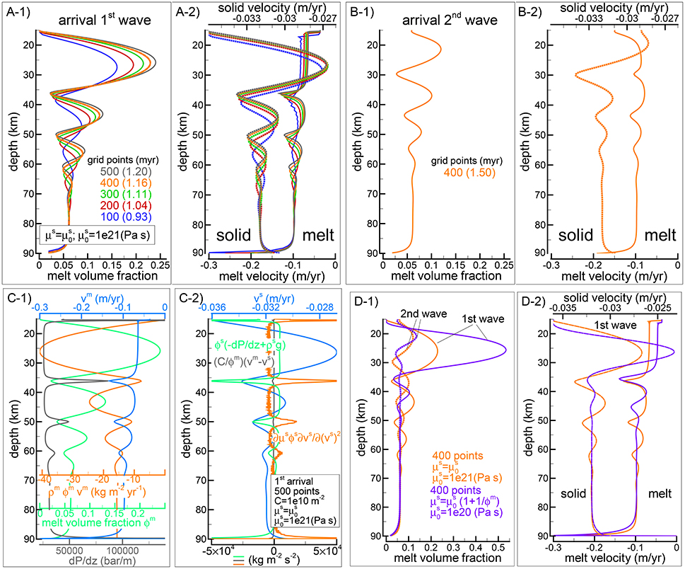
Figure 2. Dynamic two-phase flow model without thermodynamics. (A-1,A-2) Describe the melt volume fraction, melt (solid lines) and solid (dotted lines) vertical velocities when the first melt-wave arrives at the top side of the model. Different colors refer to simulation using different number of spatial grid points (100, 200, 300, 400, 500). Time step is set to 250 years except for the case indicated by the dashed green line (Δt = 500years). All the simulations assume ${\mu }^s={\mu }_0^s$, the viscosity of the solid is set to ${\mu }_0^s=1e21$ Pa s. (B-1,B-2) Show the same simulation with 400 grid points when the second melt-wave arrives at the top side. The dashed lines in panel (A–1) (barely noticeable) show the result using only the MacCormack method for the melt transport. (C-1,C-2) Summarizes some key quantities related to the simulation with 500 spatial grid points at the arrival of the first melt wave (see main text for additional information). A movie for this model is available following the instructions in the Supplementary Material (movie file mf1-movie1.PHASE33B.YRC5.avi). (D) Comparison of the first and second wave arrival at the top between the previous simulation with ${\mu }^s={\mu }_0^s=1e21$ Pa s and the one with the alternative viscosity model, ${\mu }^s={\mu }_0^s(1+1/{\varphi }^m)$, ${\mu }_0^s=1e20$ Pa s (400 grid points for both models).

The movie file mf1-movie1.PHASE33B.YRC5.avi that can be downloaded following a link to a data repository provided in the Supplementary Material, shows the time evolution and vertical variation of melt abundance, melt and solid velocity computed with the first model (${\mu }^s={\mu }_0^s$).

Thermodynamic Computation

The importance of adding the thermodynamic computation is twofold. It defines some of the parameters that are used to constrain the dynamic model. It also provides the petrological results that could be compared with geochemical or petrological field observations. When the dynamic model is interfaced with chemical thermodynamics, the essential input quantities necessary to run the thermodynamic model are not arbitrarily defined by the user, but they are obtained directly from the solution of the transport model.

The necessary data required to perform a chemical equilibrium computation based on thermodynamic principles are pressure, temperature and bulk composition of the system. At every spatial grid point these quantities are readily available from the dynamic model. Lithostatic pressure P_g computed from Equation (36) is used in this study, although the flow pressure would be the correct choice. If the dynamic pressure does not represent the pressure of the system but the interfacial pressure between melt and solid, then further assumptions should be made. However, beside more rigorous justifications, P_g is chosen at this point mainly because it provides a more stable solution from a numerical point of view. In any case the difference between the flow pressure and the lithostatic pressure is not very large for solid Earth problems (few kbars at most). The link provided in the Supplementary Material allows to access the data files from which the difference can be evaluated for every simulation included in this study. Temperature is treated following the common practice of assuming that thermal equilibrium is established among the dynamic phases of the system.

The bulk composition of the whole system at each grid point is given by the normalized sum of the composition of all the dynamic phases: $bulkcomponentc(system)=100({\Theta }_{i,t}^{sc}+{\Theta }_{i,t}^{mc}+{\Phi }_{i,t}^w)/({\Phi }_{i,t}^s+{\Phi }_{i,t}^m+{\Phi }_{i,t}^w)$ where s,m,w stand for solid, melt, free water and ${\Phi }_{i,t}^w$ is applied only to define the bulk amount of water (c = 12). The bulk composition computed with this expression is always expressed in wt %. The total mass of al the mineral phases in chemical equilibrium that are provided in the the output of the thermodynamic model is 100 (units of grams according to AlphaMELTS). The definition of the bulk composition is critical for the outcome of the melt model because it implies that thermodynamic chemical equilibrium is achieved within a certain physical domain and temporal interval among certain dynamic phases. If a different type of equilibrium condition is imposed, a different bulk composition should be used and the outcome of the thermodynamic model would be clearly different.

The following discussion outline the information applied to the dynamic model that have been retrieved specifically after running the program AlphaMELTS. The total mass and the wt % of oxides forming the bulk composition of the residual solid are extracted from the output file solid_comp_tbl.txt. If melt is present in the system, the mass of the liquid and wt % of the oxides of the liquid are retrieved from liquid_comp_tbl.txt. Thermal expansion (combining the partial derivative of the total volume with temperature and total volume of the system) and the whole system heat capacity at constant pressure (J/K) are found in the output file system_main_tbl.txt.

Mass, volume, oxide composition and heat capacity at constant pressure are extracted for each mineral component from the output file phase_main_tbl.txt. The total volume of the solid is the sum of the volumes of all the mineral phases. When melt is present, the volume and total heat capacity are also retrieved.

If free water is present in the system, mass, volume and total heat capacity are also found in the output file phase_main_tbl.txt. If water is present in the solid and also as a free phase, the solid oxide component H₂O in the output file solid_comp_tbl.txt provides the sum of the two in wt %. The mass of the total solid also includes free water. With the AlphaMELTS option ALPHAMELTS_DO_TRACE_H2O true, nominally dry minerals may contain a certain amount of water which is treated as a separate mass from the rest of the solid. The total amount of water in wet and nominally dry minerals is a quantity that can be retrieved from mass H₂O(total solid) = input bulk H₂O(system)−mass free H₂O − mass(total melt) × melt oxide(H₂O)/100 where the first term is the input water in the system, the second term is the mass of the free water phase and the last term is the amount of water in the melt. The total mass of the solid then needs to be recalculated to include the water in the nominally dry minerals, is $mass(totalsoli{d}_R)=mass{H}_{2}O(totalsolid)+{\sum }_{i}solidoxide{|}_{i}mass(totalsolid)/100.$. As shown in this equation the sum does not involve the oxide for water in the solid which is added separately. The oxides in the solid, except water, are also recalculated solid oxide|_iR = solid oxide|_i×mass(total solid)/mass(total solid_R). The water oxide in the solid is computed using the following relation solidoxide(H₂O) = mass H₂O(totalsolid) × 100/mass(totalsolid_R). When melt is the only phase in the equilibrium assemblage and water is present in the system, it should be always verified that in the output file liquid_comp_tbl.txt melt oxide(H₂O) is not erroneously set to zero.

The density of melt (kg/m³) is retrieved by dividing the mass of the melt by the volume of melt and multiplied by 1,000. The heat capacity in 1,000 grams of melt (J/(K Kg)) is obtained by dividing the total heat capacity in melt by the total mass of melt and then multiplied by 1,000. Similar relations are applied to free water, when it is present in the equilibrium assemblage. The total density of the solid is given by the following relation: 1/density(solid) = 0.001 × ∑(volume of the mineral phases)/mass(total solid). The total heat capacity of the solid (J/(K Kg)) is: 1,000 ∑(heat capacity of the mineral phases/mass(total solid)). The volume fraction of each assemblage (solid, melt, water) can be easily computed by dividing the volume of the phase by the sum of the volumes of all the phases.

The product of the density and volume fraction for solid, melt or water computed from the thermodynamic model can be directly compared with the equivalent quantity Φ^a from the dynamic model. Any difference between the two indicates that a certain amount of mass transfer has taken place. For example, the mass transfer of melt ΔΦ^m can be compute using the following relation: ΔΦ^m = [(density of the melt × volume fraction of the melt) − Φ^m], clearly when new melt is formed, ΔΦ^m > 0, conversely the solid mass transfer will be negative, ΔΦ^s < 0. Similar to the total mass transfer, the chemical mass transfer in solid and melt is defined as: ΔΘ^ac = [(density of phase a × volume fraction of phase a × bulk composition of oxide c in phase a) − Θ^ac], where a = s, m. The change of the density and heat capacity after chemical equilibration can be determined by the difference between the density and heat capacity from the thermodynamic model and density and heat capacity used in the dynamic model that were defined in the previous thermodynamic computation.

A question that may arise is how often the thermodynamic computation should be applied? In the DEM model the chemical equilibration is assumed at a scale defined by the numerical grid size, however the timescale remains undefined. A long time interval between two thermodynamic computations does not mean that the local system is completely out of equilibrium. The chemical and mass transfer ΔΦ^s and ΔΘ^al computed during the previous thermodynamic calculation still apply, although they are maintained constant over a longer period of time. For example if the thermodynamic computation is performed every 10 time steps, ΔΦ^s/10 and ΔΘ^ac/10 are applied to the dynamic model for 10 time steps. Ignoring the potential effects of dynamic changes of the local system (e.g., bulk composition, temperature) on the mass and chemical transfer over a large period of time may have some consequences. Various simulations have been performed considering a range of time step intervals between thermodynamic calculations. With time intervals ranging between 2 and 32, the results in general appear to be very similar suggesting that local dynamic changes have a small influence on the chemical and mass transfer properties. However in the Supplementary Material a plot for one particular simulation illustrates the potential effect of varying the interval between thermodynamic computations on the composition of melt (Figure S1). A more thorough comparison can be made by retrieving the data of all the simulations performed for this study following the instructions provided in the Supplementary Material.

While only the petrological information needed by the dynamic model are considered in this study, AlphaMELTS includes additional tools to evaluate trace elements and isotopes composition based on equilibrium principles. These geochemical data do not directly affect the dynamic evolution but they could be useful to provide additional constraints to the melt model by comparing the results with real observations. It is only mentioned here that each new chemical component would need additional transport equations similar to Equation (6) and new set of chemical transfers similar to those discussed in this section (e.g., ΔΘ^ac).

Results from the Dynamic Equilibrium Melting Model

The simplest dynamic melt model which also includes the thermodynamic formulation assumes the same velocity for the solid assemblage and melt. Practically it means that Equations (4) and (28) could be ignored. This type of melt model has been defined earlier dynamic batch melting. While this model probably describes an unlikely physical scenario, it cannot be dismissed a priori. For example when melt does not focus in larger channels but instead it remains in small poorly connected veins, the transport of melt may follow closely the dynamics of the mantle (e.g., big permeability constant C means small permeability, hence υ^m ≈ υ^s, see Equation 28).

One test case is illustrated here assuming only a specific set of conditions and parameters. The viscosity of the solid is constant and equal to 1e21 Pa s. Like all the models in this study, the top and bottom depth are 15 and 90 km, respectively. The model has been tested with 100, 200, and 300 spatial grid points to estimate the accuracy of the numerical solution. The time step is not fixed and it is computed using the following relation: 0.5 Δ z/|v(max)|. Lithostatic pressure at the top boundary is 5 kbar and the bottom temperature is 1,450°C. The initial temperature varies linearly from 750°C (top) to 1,300°C (bottom). It may seem arbitrary but practically it has little effect on the dynamic evolution of the model (viscosity is kept constant although the density is not). The main reason for the particular thermal profile at the starting time is to avoid the formation of extensive melting inside this initial portion of the mantle during the upwelling. Thermal conductivity for the solid and melt is set to K^s = 3 and K^m = 1 W/(m K). The velocity of the solid mantle at the bottom is fixed to −0.03 m/yr (negative upwards). While the exact origin of the imposed velocity is beyond the scope of this study, one could imagine that it is the result of thermochemical buoyancy, typically a dynamic feature of a mantle plume. The initial and bottom boundary bulk composition defining a relatively fertile mantle peridotite is: SiO₂ = 45.20, TiO₂ = 0.20, Al₂O₃ = 3.94, Fe₂O₃ = 0.20, Cr₂O₃ = 0.40, FeO = 8.10, MgO = 38.40, CaO−3.15, Na₂O = 0.41, K2O = 0, P₂O₅ = 0, H₂O = 0 in wt %. Since the solid mantle and melt have the same velocity, the bulk composition of the system does not change, provided that the initial bulk composition at every point in the model and the composition of the mantle that enters at the bottom of the model are the same and the input composition at the bottom does not vary over time. In this scenario the solution of the equation for the chemical components (Equations 6, 29, 30) would be unnecessary. Nevertheless by solving the chemical transport equations it is possible to verify the accuracy of the numerical procedure by comparing the initial bulk composition with the composition at any point in time and space computed with the relation outlined in the previous section: $bulkcomponentc(system)=100({\Theta }_{i,t}^{sc}+{\Theta }_{i,t}^{mc})/({\Phi }_{i,t}^s+{\Phi }_{i,t}^m)$ (water is ignored). The thermodynamic computation determines the local equilibrium melt and solid density, mass, and allows to determine the chemical and mass transfer properties. It also provides the heat capacity and thermal expansion of the solid and melt assemblages which are needed for the definition of the thermal field. The thermodynamic model is invoked every eight time steps. Note that because the time steps are variable, the time interval between two thermodynamic computations is not constant.

Figure 3 summarizes the results of the model after reaching a steady state condition when no further variations are observed over time. The steady state condition however does not mean that melting does not occur anymore but it simply means that the amount of melt formed locally is balanced by the amount that is mobilized by the dynamic process. Two cases are illustrated in Figure 3 which consider 300 and 100 spatial grid points (nz) and the number of time steps between thermodynamic computations is set to 8 (nthermo = 8, nthermo = 16 steps). Additional simulations performed assuming nz = 200 and nthermo = 8 and nthermo = 16 did not differ significantly from those shown in Figure 3. The results of the model with 200 grid points and nthermo = 16 time steps completely overlap with the results with 100 grid points and nthermo = 8. It is not entirely a surprise considering that the time step is defined based on the grid size and maximum velocity in the model. If the maximum velocity in the two simulation models is similar, when 200 grid points are used, the grid size is reduced by half. Hence the transported properties would cover after 16 time steps approximately the same distance that is covered by the model with 100 grid points after 8 time steps.

FIGURE 3

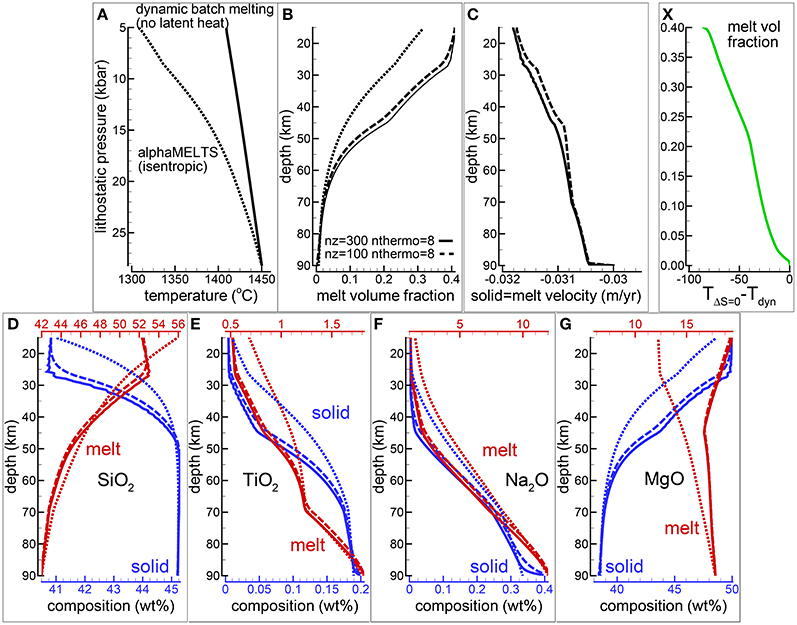
Figure 3. Dynamic batch melting, υ^melt = υ^solid. Latent heat of melting is not included in the model. (A) Temperature vs. lithostatic pressure, (B) variation of the melt volume fraction over depth, (C) solid and melt velocity, (D–G) composition of the solid and melt (wt %) (D) SiO₂, (E) TiO₂, (F) Na₂O, (G) MgO. The dotted lines show the results for an isentropic melting model using AlphaMELTS. Solid and dashed lines illustrate the results of dynamic batch melting model using different number of grid points nz = 300, 100. The number of time steps between two thermodynamic calculations (nthermo) is 8. Using nz = 100, nthermo = 8 or nz = 200, nthermo = 16 the results are very similar and they are not included in the plot. (X) Quantifies the temperature difference between the dynamic batch melting and the isentropic model as a function of the melt volume fraction obtained using the dynamic batch melting model. A movie of a dynamic batch melting simulation is available following the link provided in the Supplementary Material (movie file mf1-movie2.PHASE3-P.BRC4-5.avi).

For completeness Figure 3 reports also the results of an isentropic melting model computed with AlphaMELTS. The differences between the two models are almost entirely due to the absence of the latent heat of melt in the dynamic batch melting model. It is evident that when large amount of melt is formed under isentropic conditions the latent heat effect on the thermal profile, and consequently on the melt composition, can be quite substantial. However the general trends illustrated in Figures 3D–G for SiO₂, TiO₂, Na₂O and MgO in melt and solid are not too dissimilar, in particular for the incompatible components but also for SiO₂ in melt. Figure 3X shows that the temperature difference between the two models follows approximately a linear relation with the amount of melt obtained from the dynamic batch melting model.

The Supplementary Material provides a data repository link to access the movie (file mf1-movie2.PHASE3-P.BRC4-5.avi) showing the behavior of various melt properties along the vertical column over time computed with the dynamic batch melting model (300 spatial grid points and nthermo = 8). The data file PHASE3-P.BRC4-5.DAT (zip file max-front1-data.zip) related to the animation can be also retrieved following the link in the Supplementary Material. See the Supplementary Material for a description of the data file.

The fully implementation of the model presented in this study includes a two-phase flow transport model that is coupled with the thermodynamic computation performed at every spatial grid point and at variable time intervals. Figure 4 illustrates some of the results of one model that belongs to a group of several simulations with the viscosity of the solid matrix defined by the relation ${\mu }^s={\mu }_0^s$. As discussed in section “Description of the Multiphase Dynamic Model” the variation of the viscous forces in 1-D is described by a simplified expression, ∂μ^sϕ^s∂υ^s/∂z². Various conditions have been tested by several numerical models, in particular the effect of the solid viscosity without melt ${\mu }_0^s$ and the permeability parameter C. A complete list of all the simulations is reported in Table 1 and the data files of most of the listed simulations are accessible following the instructions provided in the Supplementary Material (zip file max-front1-data.zip). Parameters not specified in the table, in particular related to the initial and boundary conditions, are similar to those used for the batch dynamic melt model discussed earlier. The model shown in Figure 4 is particularly interesting because the melt variation with depth never reaches a steady condition, Figure 4A illustrates the point by reporting the melt distribution at three different times. Another noteworthy feature is that the first melt arrival a the top of the model after ~2.09 Myr is characterized by the largest volume fraction, a similar behavior was observed in the simple dynamic model reported in Figure 2.

TABLE 1

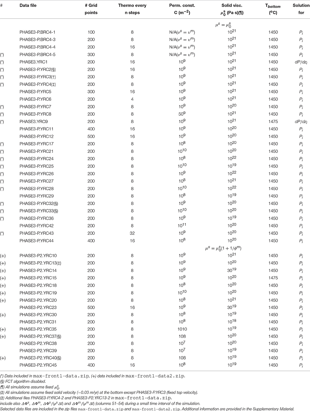
Table 1. List of the dynamic melting simulations with thermodynamic computation.

FIGURE 4

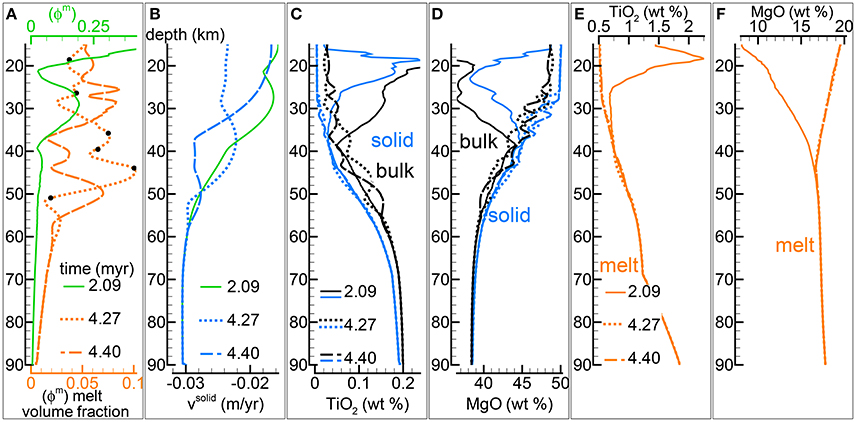
Figure 4. Two-phase flow dynamic melting with thermodynamic computation applied every 8 time steps, solid viscosity model: ${\mu }^s={\mu }_0^s$ with ${\mu }_0^s$, equal to 1e21 Pa s. Additional details related to this simulation are discussed in section “Results from the Dynamic Equilibrium Melting Model.” (A) Melt volume fraction vs. depth at 3 different times. Earliest time corresponds approximately to the first arrival of melt at the top. Black dots mark the locations at which mineralogical compositions and volume fractions are reported in Table 2. (B) Velocity of the solid matrix. (C) Variation of TiO₂ in solid and bulk (melt + solid) (wt %). (D) Variation of MgO in solid and bulk (melt + solid) (wt %). (E) Variation of TiO₂ in melt (wt %). (F) Variation of MgO in melt (wt %). The complete data for all 12 oxides in melt solid and bulk, at every depth over time can be found in the data file PHASE3-P.YRC4.DAT (zip file max-front1-data.zip). A movie of this simulation is also available (movie file mf1-movie3.PHASE3-P.YRC4.avi). Both files can be retrieved following the data repository link included in the Supplementary Material.

It was previously mentioned that the thermal effect of the latent heat of melting has been neglected in the thermal model. The contribution can be significant when large amount of melt is created under isentropic conditions which can be achieved essentially when υ^s = υ^m. In a two-phase flow model the velocity of the melt and the solid are not the same and the isentropic condition is not maintained but the latent heat still has a role on the definition of the thermal profile. However since the amount of melt that is locally formed is substantially lower than in a dynamic batch melting (or isentropic) model, it is possible to approximately estimate from Figure 3X that the temperature is overestimated by no more than few tens of degrees.

Figure 4B shows that there is no direct correlation between the melt distribution and the velocity of the residual solid although, as expected, the broad effect of the melt is to reduce the upwelling velocity of the mantle (velocity negative upwards). The numerical simulation includes the complete chemical evolution of the solid residual mantle and the melt over time at every depth point. Figures 4C,D report just two components, TiO₂ and MgO (wt %). Except for the first melt arrival, the temporal variation of the melt abundance seems to have a negligible influence on the composition of the melt and a small effect on the variation of the composition of the residual solid (and bulk composition). The general variations of the chemical components in the melt and solid with depth are also very similar to the variations observed in the dynamic batch melting model, which is quite remarkable considering the large difference in the melt distribution between the two models and the change of the bulk composition with depth. The implication is that the interpretation of petrological observations can be assumed to be rather independent from the dynamic evolution of the melting process. The drawback is that real petrological data may not be able to provide a robust insight on these processes. The results for all twelve oxide components are reported in the data file PHASE3-P.YRC4.DAT included in the zip file max-front1-data.zip. Details to retrieve a movie of the DEM simulation can be found in the Supplementary Material (mf1-movie3.PHASE3-P.YRC4.avi).

Not all the information created by the simulations have been saved in the output data files. The thermodynamic calculation provides the complete mineralogy of the solid mantle at equilibrium at every spatial grid point over time. This information is not included in the output files that store only the essential data: melt, whole solid and bulk (melt +solid) composition. However with these data after the dynamic simulation is completed, it is possible to re-calculate the mineralogical assemblage at any point from the output data file using AlphaMELTS. This is shown for example in Table 2 where the mineral composition at six depth locations denoted by black dots in Figure 4A has been computed using the bulk composition, temperature and pressure stored in the data file PHASE3-P.YRC4.DAT (point#: 12, 36, 58, 69, 80, 99. Zone: 5111). In accordance with the variation of the residual solid composition, the results reported in the table suggests that minerals occurrence and their abundance don't seem to be related to the variations of the melt fraction with depth.

TABLE 2

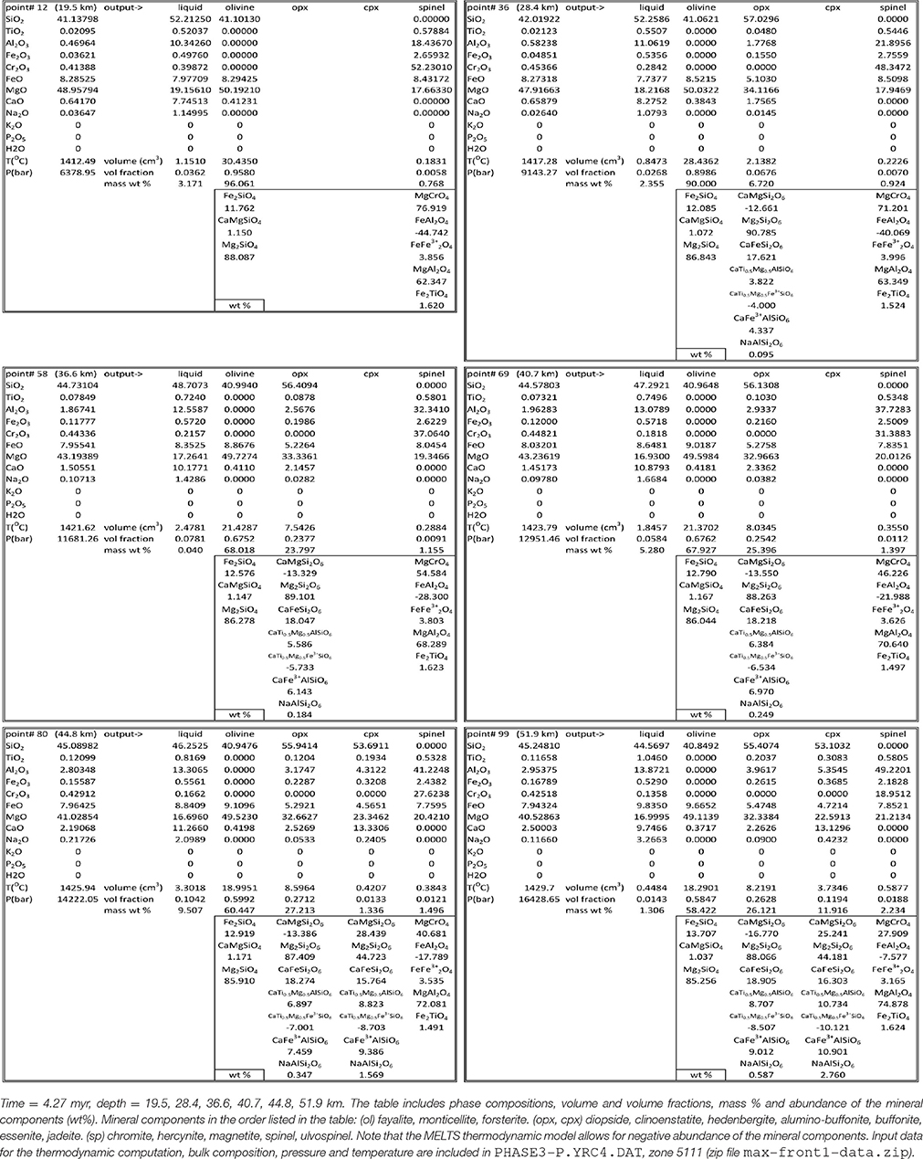
Table 2. Mineral data at 6 depths for the model shown in Figure 4.

In section “Description of the Multiphase Dynamic Model” it was mentioned that the solid viscosity may depend also on the inverse of the melt abundance and the following equation was proposed ${\mu }^s={\mu }_0^s(1+1/{\varphi }^m)$. Several numerical simulations have been performed with this description of the viscosity (Table 1), an example of the outcome is presented in Figure 5. One general observation is that, for the range of conditions applied to the various numerical models, the melt distribution with depth tends to always reach a time-invariant condition. The first melt arrival (Figure 5A) time~2.1 Myr) is characterized by large volumes, a similar development has been also observed in the previous model shown in Figure 4. After the arrival of the first melt wave (Figure 4A) time~3.2 Myr), the melt distribution shows little variation with time. The animation mf1-movie4.PHASE3-P2.YRC13.avi that can be found following the instructions in the Supplementary Material clearly illustrates the point. The time invariant melt distribution defines two inversions of the gradient with depth that occur at ~45 km and ~27 km depth. In Figures 4C,D it is shown that only MgO in the solid correlates with the melt distribution while the other components in the solid and all the components in the melt seem to follow a pattern unrelated to the melt and its slope inversions. The compositional difference between the first melt arrival and later melt advancements is quite significant. It can be also observed that in the near steady state regime the composition of the solid and melt is very similar to the composition observed in the previous models (Figures 3, 4).

FIGURE 5

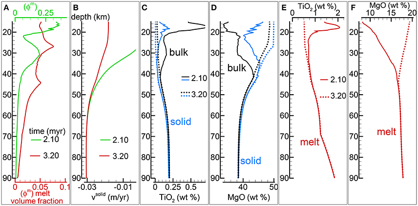
Figure 5. Two-phase flow dynamic melting with thermodynamic computation applied every 8 time steps, solid viscosity model: ${\mu }^s={\mu }_0^s(1+1/{\varphi }^m)$ with ${\mu }_0^s=1e20$ Pa s. Additional details related to this simulation are discussed in section “Results from the Dynamic Equilibrium Melting Model.” (A) Melt volume fraction vs. depth at 2 different times. Earliest time indicates approximately the first arrival of melt at the top. (B) Velocity of the solid matrix. (C) Variation of TiO₂ in solid and bulk (melt + solid) (wt %). (D) Variation of MgO in solid and bulk (melt + solid) (wt %). (E) Variation of TiO₂ in melt (wt %). (F) Variation of MgO in melt (wt %). The complete data for all 12 oxides in melt solid and bulk, at every depth over time are included in the data file PHASE3-P2.YRC13.DAT (zip file max-front1-data2.zip). A movie of this simulation is available (movie file mf1-movie4.PHASE3-P2.YRC13.avi). The instructions to retrieve both files are provided in the Supplementary Material.

The presence of one or more inversion points where the gradient with depth of the melt volume fraction turns from negative to positive is a recurrent feature of many simulations carried out for this study. The first impression is that the inversion is simply due to a change of the mass transfer rate, that is the mantle regime changes from partial melting to partial crystallization. However the inspection of the data files, for example PHASE3-P.YRC4-2.DAT, reveals that the melt transfer ΔΦ^m is always positive at any depth, which implies that no crystallization is taking place. Predicting this melt behavior based on the model setup may not be possible, however the dynamic factors that control the inversion can be analyzed. The equation of motion for melt −ϕ^m∂P/∂z + ϕ^mρ^mg−ϕ^m2/k^m(υ^m−υ^s) = 0 (Equation 3) can be rearranged as follows: −ϕ^m2∂P/∂z + ϕ^m2ρ^mg − C(υ^m−υ^s) = 0 where k^m = ϕ^m3/C and water is not present. By taking the partial derivative with respect to depth and after some rearrangements, the following expression is obtained:

$\begin{array}{ll}\frac{\partial {\varphi }^m}{\partial z}=\frac{{\varphi }^{m^2}\frac{{\partial }^{2}P}{\partial z^2}+C\left(\frac{\partial {\upsilon }^m}{\partial z}-\frac{\partial {\upsilon }^s}{\partial z}\right)-{\varphi }^{m^2}g\frac{\partial {\rho }^m}{\partial z}}{2{\varphi }^m\left(-\frac{\partial P}{\partial z}+{\rho }^{m}g\right)}\hfill & (37)\hfill \end{array}$

If we consider the denominator on the rhs as a scaling factor, the equation allows to determine the condition at which the inversion of the melt gradient may occur, that is when ∂ϕ^m/∂z = 0. Figure 6A-1) includes, along with the melt distribution for the simulation presented in Figure 4, the scaled ∂ϕ^m/∂z computed using Equation (37). The black dots highlight some of the inversion points where ∂ϕ^m/∂z is zero. Figure 6A-2 illustrates the three components forming the scaled gradient of the melt fraction defined on the rhs of Equation (37). The third component ϕ^m2g∂ρ^m/∂z is rather small but the other two are comparable. The interesting observation is that the condition ∂ϕ^m/∂z = 0 is not obtained by self-cancellation of the two dominant terms but instead all terms are zero at the inversion points. While the dynamic coupling effect between melt and solid exemplified by the permeability constant C is explicitly included in Equation (37), the effect of the viscous forces is not quite clear. Considering the total equation of motion −∂P/∂z + ϕ^mρ^mg + ϕ^sρ^sg+S = 0 (Equation 5), by taking the partial derivative with respect to depth, the following expression can be found:

$\begin{array}{ll}\frac{{\partial }^{2}P}{\partial z^2}=\frac{\partial S}{\partial z}+g\frac{\partial {\varphi }^m}{\partial z}\left({\rho }^m-{\rho }^s\right)+{\varphi }^{m}g\frac{\partial {\rho }^m}{\partial z}+{\varphi }^{s}g\frac{\partial {\rho }^s}{\partial z}\hfill & (38)\hfill \end{array}$

where the relation ∂ϕ^m/∂z = −∂ϕ^s/∂z has been applied. The above relation provides the connection between the derivative of the variation of the viscous forces and the derivative of the pressure gradient which also appears on the rhs of Equation (37). A further consideration can be made. If the viscous forces are not included in the description of the melting process (S is ignored, hence ∂S/∂z = 0), an inversion point could not appear because if ∂ϕ^m/∂z was zero, then from Equation (38) the derivative of the pressure gradient would be ∂²P/∂z² = ϕ^mg∂ρ^m/∂z + ϕ^sg∂ρ^s/∂z, which could never be zero, unless the density of melt and solid are assumed to be constant.

FIGURE 6

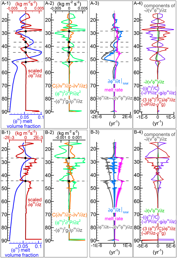
Figure 6. Flow analysis of the simulations shown in Figures 4, 5. (A-1–A-4) Refer to the model with ${\mu }^s={\mu }_0^s$ and ${\mu }_0^s=1e21$ Pa s. (A-1) Variation with depth of the melt fraction at 4.27 Myr and scaled ∂ϕ^m/∂z which characterizes the inversion point at ∂ϕ^m/∂z = 0. (A-2) The three components defining the scaled ∂ϕ^m/∂z. (A-3) Temporal variation of the melt fraction. The total variation $\partial {\varphi }^m/\partial t{|}_{total}$ is the sum of −∂(ϕ^mv^m)/∂z ≈ ∂ϕ^m/∂t and the melting rate retrieved from the thermodynamic and dynamic models (see section Thermodynamic Computation). (A-4) Components forming −∂(v^mϕ^m/∂z. See section “Results from the Dynamic Equilibrium Melting Model” for a discussion of these quantities. (B-1–B-4) same as (A-1–A-4) but for the model with ${\mu }^s={\mu }_0^s(1+1/{\varphi }^m)$ and ${\mu }_0^s=1e20$ Pa s that is shown in Figure 5 at 3.2 Myr.

In some cases the numerical models show that the melt variation with depth is time dependent. To understand the nature of such behavior and how it is related to the viscous forces and the dynamic coupling term or the permeability constant, the equation of motion for melt can be written as follows: −ϕ^m3 ∂P/∂z + ϕ^m3ρ^mg − Cϕ^mυ^m + Cϕ^mυ^s = 0, where water is not considered. By taking the partial derivative with respect to depth and after some rearrangements:

$\begin{array}{ll}\begin{array}{l}-\frac{\partial ({\varphi }^m{\upsilon }^m)}{\partial z}=-\frac{3{\varphi }^{m^2}}{C}\frac{\partial {\varphi }^m}{\partial z}\left(-\frac{\partial P}{\partial z}+{\rho }^{m}g\right)\\ -\frac{{\varphi }^{m^3}}{C}\left(-\frac{{\partial }^{2}P}{\partial z^2}+g\frac{\partial {\rho }^m}{\partial z}\right)-\frac{\partial ({\varphi }^m{\upsilon }^s)}{\partial z}\end{array}\hfill & (39)\hfill \end{array}$

which is simply an alternative for the expression given in Equation (37). However in this form it can be related to the change of the melt volume fraction over time, using the mass conservation equation. Assuming ϕ^m∂ρ^m/∂t and ϕ^mυ^m∂ρ^m/∂z to be negligible, the following approximation of the mass conservation equation ∂ϕ^m/∂t ≈ −∂(ϕ^mυ^m)/∂z provides the connection between the temporal variation of the volume fraction and the dynamic parameters given in Equation (39). Note that the variation of the melt abundance by melting (or crystallization) is not included, hence the melting rate needs to be added in order to find $\partial {\varphi }^m/\partial t_{total}$. Figure 6A-3 shows the total melt variation over time and the two components that form it. Since the melt production (positive melting rate) does not compensate for the change of the melt flux, the amount of melt is expected to vary over time. The three components defining the variation of the melt flux which can be related to the physical properties of the model (Equation 39), are shown in Figure 6A-4). The first and second term on the rhs of Equation (39) are clearly the largest but they have opposite sign and they tend to cancel out. The same analysis can be applied to the model that assumes ${\mu }^s={\mu }_0^s(1+1/{\varphi }^m)$ (Figures 6B-1–B-4). In this case the local melt production compensates the variation of the melt flux, hence $\partial {\varphi }^m/\partial t_{total}$ is close to zero at any depth and a condition of dynamic steady state is observed.

The model presented in this study opens up the possibility of a comparison with real petrological data. For this purpose perhaps the most useful result from the simulations is the composition and the amount of the melt at the exit point, that is the point of extraction at the top of the mantle column. Figure 7 illustrates the variation over time of the melt flux, melt velocity, and three melt components, SiO₂, MgO and CaO at the extraction point. The results of three models are included. The main difference is the viscosity of the solid without melt (${\mu }_0^s$) which is set to 10²⁰, 10²¹ and 10²² Pa s. The three models assume ${\mu }^s={\mu }_0^s$ and permeability constant C = 10⁻⁹ m⁻². In addition the results of the dynamic batch melting model (υ^s = υ^m, 300 grid points) are also included for reference. The main differences that can be observed between the batch melting model and the three DEM models are mainly related to the first melt arrival. Once the melt column is fully developed, periodic oscillations are clearly visible for the model with ${\mu }_0^s=10^{21}$. Complete data sets related to these models can be found in the zip file max-front1-data.zip, data files: PHASE3-P.BRC4-5.DAT, PHASE3-P.YRC7.DAT, PHASE3-P.YRC3.DAT and PHASE3-P.YRC26.DAT (for additional information see Table 1 and Supplementary Material).

FIGURE 7

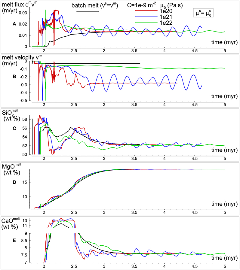
Figure 7. Variation of selected melt properties over time at the top side (exit point) of the simulation for three models with ${\mu }^s={\mu }_0^s$. The permeability constant is C=10⁻⁹ m⁻², ${\mu }_0^s$ is set to 10²⁰, 10²¹, 10²² Pa s. Results from the batch melting model are also included. (A) The melt flux (ϕ^mv^m) shows the amount of melt per year that is extracted from the mantle column. (B) Melt velocity (m/yr). (C) Melt composition: SiO₂ (wt %). (D) Melt composition: MgO (wt %). (E) Melt composition: CaO (wt %). Complete data can be found in PHASE3-P.BRC4-5.DAT, PHASE3-P.YRC7.DAT, PHASE3-P.YRC4.DAT, and PHASE3-P.YRC26.DAT (zip file max-front1-data.zip).

The same plot is also shown for three simulations that assume ${\mu }^s={\mu }_0^s(1+1/{\varphi }^m)$ with ${\mu }_0^s$ equal to 10¹⁹, 10²⁰ and 10²¹ Pa s and permeability constant C equal to 10⁻⁹ m⁻² (Figure 8). After the arrival of the first melt wave, the melt flux and melt composition approach the values found for the batch melting model. The complete data sets included in the zip file max-front1-data2.zip are: PHASE3-P2.YRC14.DAT, PHASE3-P.YRC13.DAT and PHASE3-P.YRC10.DAT.

FIGURE 8

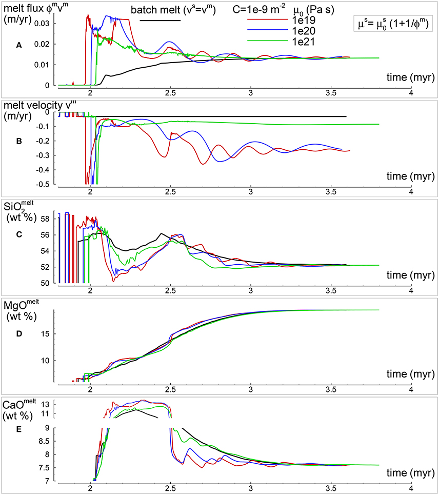
Figure 8. Variation of selected melt properties over time at the top side of the simulation for three models with ${\mu }^s={\mu }_0^s(1+1/{\varphi }^m)$. The permeability constant is C = 10⁻⁹ m⁻², ${\mu }_0^s$ is set to 10¹⁹, 10²⁰, 10²¹ Pa s. For comparison the results from the batch melting model are also reported in the plot. (A) Melt flux (ϕ^mv^m). (B) Melt velocity (m/yr). (C) Melt composition: SiO₂ (wt %). (D) Melt composition: MgO (wt %). (E) Melt composition: CaO (wt %). Complete data can be found in PHASE3-P.BRC4-5.DAT, PHASE3-P2.YRC14.DAT, PHASE3-P2.YRC13.DAT and PHASE3-P2.YRC10.DAT (zip file max-front1-data2.zip).

While the results of different models appear to be similar, it may be worth to comment on the implications regarding the thermodynamic equilibrium assumption. Considering two cases with similar flux, in one case the melt velocity is low and the melt abundance is high, it means that chemical equilibrium with the residual solid is imposed on large amount of melt moving slower. In the other case the melt velocity is comparably higher and the melt abundance is lower, in other words smaller amount of melt moving faster is also chemically equilibrated with the residual solid. Clearly these are two different physical scenarios but it is still unclear which one in reality may approach closer the imposed condition of thermodynamic equilibrium. The difference between the two cases becomes even more significant considering that the time step in the simulations depends on the inverse of the maximum velocity. If the applied number of time steps defining the interval between two thermodynamic calculations is the same, then in the first case the time step would be larger hence thermodynamic equilibrium would be assumed to be achieved over a longer period of time.

Discussion and Conclusions

It is common to use petrological data (mainly geochemical data) to investigate some aspects of the Earth's interior and the processes that led to the formation and evolution of igneous and metamorphic rocks. However simple models not necessarily very realistic are often applied to explain how the conditions in the Earth's interior influence the petrological evolution and how these processes affect the geochemical signature.

This work, which is an extension of a previous study (Asimow and Stolper, 1999), begins to address the petrological evolution of mantle melting combining perhaps the most well-calibrated thermodynamic model for melt developed by Ghiorso with a multiphase transport model. The main motivation is to try to understand how the melt dynamics affect the petrology and geochemistry of igneous rocks. The model presented here is based on a 1-D mantle column defined in a restricted pressure range. The limitations are mainly dictated by the thermodynamic model. The attractive point of using a 1-D model interfaced with an accurate petrological description rather than a 2-D or 3-D dynamic model with a simplified petrological representation is that it becomes possible to make a better comparison with real petrological data. The limitation of a 1-D model however implies that the description of the melting process is restricted to the vertical axis of a plume or a mid-ocean ridge, hence lateral melt focusing and other lateral variations are effectively ignored. If a new version of the thermodynamic melt model with expanded pressure range will become available, the effect of viscous dissipation on temperature transport Equation (7) may become significant (Tirone, 2016) and should be included. It is still a challenging task to include the contribution of chemical transformations to the temperature equation because the required self-consistency with the variation of melt production with temperature. For two-phase flow models the effect may not be too dramatic and possibly limited to few tens of degrees.

Only a small set of parameters (mainly related to the permeability and the rheology of the solid mantle) were varied for this study. The input composition at the bottom of the mantle column is assumed to be homogeneous over time and to represent a fertile peridotite. An heterogeneous mantle has been considered elsewhere (Katz and Weatherley, 2012). However without convincing arguments, even the assumption of a chemical heterogeneous mantle in local equilibrium (Tirone et al., 2015) may require further investigation.

In this first installment it was only considered the scenario in which the melt and the residual solid are always in thermodynamic equilibrium within a finite volume in space and time interval. In a certain way the idea replicates the traditional petrological approach of assuming a batch melting. The clear improvement is that with the dynamic equilibrium melting model (DEM) introduced in this study, the process is located in space and time. It is therefore possible to follow the melt evolution and how certain conditions (e.g., temperature, upwelling velocity) may or may not affect the outcome. From a dynamic point of view, the association of melt porous flow with a thermodynamic model seems to be reasonable because in the porous flow regime the minerals surface in contact with melt would be large, hence it would become easier to establish chemical equilibrium between the solid and the melt. The obvious question is whether the DEM model describes with some degree of confidence the reality of a process that occurs in the Earth's interior where melt velocity and abundance can vary considerably. The answer cannot be found here but perhaps once the model is applied to specific geological problems a more clear picture will emerge.

Understanding the nature of the rheological interaction between the solid mantle and melt is beyond the scope of this study, it is a problem that pertains to theoretical or perhaps experimental fields. Here it is merely shown what would be the consequence of adopting a certain function for the bulk (dilatational) viscosity or ignore its effect.

The solution of the set of dynamic equations that are needed to address the melting process may seem difficult even for a 1-D problem. In previous studies usually very few details on the numerical procedure are provided. Certain simplifications have been also applied, for instance regarding the variation of the density (e.g., Schmeling, 2000). The numerical scheme presented in this study should be relatively easy to follow and does not rely on simplifications. The output data files for most of the simulations are available following the data repository link provided in the Supplementary Material. Independent browsing of the data may help to unravel features of the melt model not specifically discussed here. In addition the data may be helpful for a comparison of the results with alternative and perhaps better numerical procedures. The implementation of the FCT algorithm presented in Appendix 1 (Supplementary Material), has provided a better numerical solution in certain situations (see for example a comparison between the results in PHASE3-P.YRC7.DAT and PHASE3-P.YRC32.DAT or between PHASE3-P.YRC21.DAT and PHASE3-P.YRC33.DAT).

One of the results from the application of the DEM model is that the first melt arrival is characterized by a large volume and that the composition is quite different from the composition of later melt products. It appears to be a consistent observation within the conditions imposed to the model. This melt behavior which has been also discussed in previous studies, although for a different model setup (Spiegelman, 1993b), is a direct consequence of the physical (not petrological) nature of the two-phase melt model. The possible connection with the formation of large igneous provinces and emplacement of flood basalts or oceanic plateaus (e.g., White and McKenzie, 1989; Kerr and Mahoney, 2007) with or without the presence of a thermal plume seems to be quite reasonable. The comparison of several DEM simulations at different conditions suggests that the melt distribution with depth is significantly affected by the permeability and viscosity of the solid rocks. It also appears that the composition of the melt computed with the two-phase flow model is not significantly different than the composition obtained from a dynamic batch melt model where υ^s = υ^m. Some variations may still be observed, in particular when the melt distribution changes with time. The implication is that a more complex dynamic melt model like the DEM may not be always necessary to describe the petrological evolution of melt under the assumption of local thermodynamic equilibrium. Although a two-phase flow model would be still necessary in order to quantify the melt abundance. It also implies that geochemical or petrological data may not be the most reliable source of information to discern the dynamic of the melt process, at least after the first melt arrival. However before drawing major conclusions more work would be needed, in particular to explore the effect of the temperature, initial mantle composition and the velocity of the mantle imposed at the boundary of the model. Regarding this last point, all the simulations presented in this study (with one exception, see Table 1) assumes a fixed velocity of the mantle at the bottom of the 1-D column, essentially considering a condition of active flow that can be imagined to be the result of a thermochemical mantle plume. In alternative the boundary condition that assumes an imposed velocity at the top of the mantle column may represent instead a passive flow. For example it could be the result of pulling forces which are dominant in mid-ocean ridges. The two scenarios, although similar (i.e., mantle moving upwards), may lead to different results.

Author Contributions

JS developed the initial version of the program used in this study for a petrology project while pursuing his Ms degree at the Ruhr-Universität Bochum, Institut für Geologie, Mineralogie und Geophysik. JS successfully implemented the procedure to interface the program AlphaMELTS with a dynamic model that, for his Ms project, involved only melt transport (Darcy flow). MT outlined the general idea for this study, made the necessary modifications to the earlier version of the program and finalized the work in the form that is presented here. MT is the solely responsible for any mistake or miscalculation that may have affected the model and the results.

Conflict of Interest Statement

The authors declare that the research was conducted in the absence of any commercial or financial relationships that could be construed as a potential conflict of interest.

Acknowledgments

Thanks to Paula Smith for fixing a small glitch in the program AlphaMELTS (version 1.7) and for clarifying certain aspects of the output files. The manuscript was prepared while MT was visiting the Department of Mathematics and Geosciences at the University of Trieste, Italy. I am truly grateful to the reviewers for their insightful comments that greatly improved the manuscript in several ways.

Supplementary Material

The Supplementary Material for this article can be found online at: https://www.frontiersin.org/articles/10.3389/feart.2017.00081/full#supplementary-material

References

Abreu, E., Douglas, J. Jr., Furtado, F., Marchesin, D., and Pereira, F. (2006). Three-phase immiscible displacement in heterogeneous petroleum reservoirs. Math. Comput. Simulat. 73, 2–20. doi: 10.1016/j.matcom.2006.06.018

CrossRef Full Text | Google Scholar

Asimow, P. D. (2002). Steady state mantle-melt interaction in one dimension: II. Thermal interactions and irreversible terms. J. Petrol. 43, 1707–1724. doi: 10.1093/petrology/43.9.1707

CrossRef Full Text | Google Scholar

Asimow, P. D., and Stolper, E. M. (1999). Steady-state mantle-melt interactions in one dimension: I. Equilibrium transport and melt focusing. J. Petrol. 40, 475–494. doi: 10.1093/petroj/40.3.475

CrossRef Full Text | Google Scholar

Bercovici, D., and Ricard, Y. (2003). Energetics of a two-phase model of lithospheric damage, shear localization and plate boundary formation. Geophys. J. Int. 152, 581–596. doi: 10.1046/j.1365-246X.2003.01854.x

CrossRef Full Text | Google Scholar

Bercovici, D., Ricard, Y., and Schubert, G. (2001). A two-phase model for compaction and damage, part 1: general theory. J. geophys. Res. 106, 8887–8906. doi: 10.1029/2000JB900430

CrossRef Full Text | Google Scholar

Bird, R. B., and Stewart, W. E. Lightfoot E. N. (2002). Transport Phenomena. 2nd Edn. New York; London: John Wiley & Sons, Inc.

Book, D. L., and Boris, J. P. (1975). Flux-corrected transport II: Generalizations of the Method. J. Comput. Phys. 18, 248–283. doi: 10.1016/0021-9991(75)90002-9

CrossRef Full Text | Google Scholar

Boris, J. P., and Book, D. L. (1973). Flux-corrected transport. I. SHASTA, a fluid transport algorithm that works. J. Comput. Phys. 11, 38–69. doi: 10.1016/0021-9991(73)90147-2

CrossRef Full Text | Google Scholar

Cordery, M. J., and Morgan, J. P. (1993). Convection and melting at mid-ocean ridges. J. Geophys. Res. 98, 19477–19503. doi: 10.1029/93JB01831

CrossRef Full Text | Google Scholar

Corey, A. T., Rathjens, C. H., Henderson, J. H., and Wyllie, M. R. (1956). Three-phase relative permeability. Trans. AIME 207, 349–351. doi: 10.2118/737-G

CrossRef Full Text

Dria, D. E., Pope, G. A., and Sepehrnoorl, K. (1993). Three-phase gas/oil/brine relative permeabilities measured under CO₂ flooding conditions. SPE Reservoir. Eng. 8, 143–150. doi: 10.2118/20184-PA

CrossRef Full Text | Google Scholar

Ghiorso, M. S. (1985). Chemical mass transfer in magmatic processes I. Thermodynamic relations and numerical algorithms. Contrib. Mineral. Petrol. 90, 107–120. doi: 10.1007/BF00378254

CrossRef Full Text | Google Scholar

Ghiorso, M. S., and Sack, R. O. (1995). Chemical mass transfer in magmatic processes IV. A revised and internally consistent thermodynamic model for the interpolation and extrapolation of liquid-solid equilibria in magmatic systems at elevated temperatures and pressures. Contrib. Mineral. Petrol. 119, 197–212. doi: 10.1007/BF00307281

CrossRef Full Text | Google Scholar

Ghiorso, M. S., Hirschmann, M. M., Reiners, P. W., and Kress, V. C. III (2002). The pMELTS: a revision of MELTS for improved calculation of phase relations and major element partitioning related to partial melting of the mantle to 3 GPa. Geochem. Geophys. Geosys. 5:1030. doi: 10.1029/2001GC000217

CrossRef Full Text | Google Scholar

Ghods, A., and Arkani-Hamed, J. (2000). Melt migration beneath mid-ocean ridges. Geophys. J. Int. 140, 687–697. doi: 10.1046/j.1365-246X.2000.00032.x

CrossRef Full Text | Google Scholar

Herzberg, C., and Asimow, P. D. (2008). Petrology of some oceanic island basalts: PRIMELT2.xls software for primary magma calculation. Geochem. Geophys. Geosyst. 9:Q09001. doi: 10.1029/2008GC002057

CrossRef Full Text | Google Scholar

Herzberg, C., Asimow, P. D., Arndt, N., Niu, Y., Lesher, C. M., Fitton, J. G., et al. (2007). Temperatures in ambient mantle and plumes: constraints from basalts, picrites, and komatiites. Geochem. Geophys. Geosyst. 8:Q02006. doi: 10.1029/2006GC001390

CrossRef Full Text | Google Scholar

Hewitt, I. J. (2010). Modelling melting rates in upwelling mantle. Earth Planet. Sci. Lett. 300, 264–274. doi: 10.1016/j.epsl.2010.10.010

CrossRef Full Text | Google Scholar

Hewitt, I. J., and Fowler, A. C. (2008). Partial melting in an upwelling mantle column. Proc. R. Soc. A 464, 2467–2491. doi: 10.1098/rspa.2008.0045

CrossRef Full Text | Google Scholar

Jennings, E. S., and Holland, J. B. (2015). A simple thermodynamic model for melting of peridotite in the system NCFMASOCr. J. Petrol 5, 869–892. doi: 10.1093/petrology/egv020

CrossRef Full Text | Google Scholar

Katz, R. F. (2008). Magma dynamics with the enthalpy method: benchmark solutions and magmatic focusing at mid-ocean ridges. J. Petrol. 49, 2099–2121. doi: 10.1093/petrology/egn058

CrossRef Full Text | Google Scholar

Katz, R. F., and Weatherley, S. M. (2012). Consequences of mantle heterogeneity for melt extraction at mid-ocean ridges. Earth Planet Sci. Lett. 335–336, 226–237. doi: 10.1016/j.epsl.2012.04.042

CrossRef Full Text | Google Scholar

Kerr, A. C., and Mahoney, J. J. (2007). Oceanic plateaus: problematic plumes, potential paradigms. Chem. Geol. 241, 332–353. doi: 10.1016/j.chemgeo.2007.01.019

CrossRef Full Text | Google Scholar

Ishii, M., and Hibiki, T. (2006). Thermo-fluid Dynamics of Two-Phase Flow. New York, NY: Springer Science+Bussiness Media Inc. doi: 10.1007/978-0-387-29187-1

CrossRef Full Text | Google Scholar

Langmuir, C. H., Klein, E. M., and Plank, T. (1992). Petrological systematics of mid-ocean ridge basalts: constraints on melt generation beneath ocean ridges, in Mantle Flow and Melt Generation at Mid-Ocean Ridges, Geophysical Monograph 71, eds J. P. Morgan, D. K. Blackman, and J. M. Sinton (Washington, DC: American Geophysical Union), 183–280. doi: 10.1029/GM071p0183

CrossRef Full Text | Google Scholar

MacCormack, R. (1969). The effect of viscosity in hypervelocity impact cratering, in 4th Aerodynamic Testing Conference, Aerodynamic Testing Conference (Cincinnati, OH). doi: 10.2514/6.1969-354

CrossRef Full Text | Google Scholar

McKenzie, D. (1984). The generation and compaction of partially molten rock. J. Petrol. 25, 713–765. doi: 10.1093/petrology/25.3.713

CrossRef Full Text | Google Scholar

Patankar, S. V. (1980). Numerical Heat Transfer and Fluid Flow. New York, NY: Hemisphere Pub. Corp., McGraw-Hill.

Google Scholar

Peaceman, D. W. (1977). Fundamentals of Numerical Reservoir Simulation, Vol. 6, Developments in Petroleum Science. New York, NY: Elsevier North-Holland Inc. 177.

Press, W. H., Flannery, B. P., Teukolosky, S. A., and Vetterling, W. T. (1992). Numerical Recipes. 2nd Edn. New York, NY: Cambridge University Press.

Richardson, C. N. (1998). Melt flow in a variable viscosity matrix. Geophys Res. Lett. 25, 1099–1102. doi: 10.1029/98GL50565

CrossRef Full Text | Google Scholar

Rudge, J. F., Bercovici, D., and Spiegelman, M. (2011). Disequilibrium melting of a two phase multicomponent mantle. Geophys. J. Int. 184, 699–718. doi: 10.1111/j.1365-246X.2010.04870.x

CrossRef Full Text | Google Scholar

Schmeling, H. (2000). Partial melting and melt segregation in a convecting mantle, in Physics and Chemistry of Partially Molten Rocks, eds N. Bagdassarov, D. Laporte, and A. B. Thompson (Dordrecht: Kluwer), 141–178.

Google Scholar

Scott, D. R., and Stevenson, D. J. (1986). Magma ascent by porous flow. J. Geophys. Res. 91, 9283–9296. doi: 10.1029/JB091iB09p09283

CrossRef Full Text | Google Scholar

Scott, D. R., and Stevenson, D. J. (1984). Magma solitons. Geophys. Res. Lett. 11, 1161–1164. doi: 10.1029/GL011i011p01161

CrossRef Full Text | Google Scholar

Simpson, G., Spiegelman, M., and Weinstein, M. I. (2010). A multiscale model of partial melts: 2. Numerical results. J. geophys. Res. 115:B04411. doi: 10.1029/2009JB006376

CrossRef Full Text | Google Scholar

Smith, P. M., and Asimow, P. D. (2005). Adiabat_1ph: a new public front-end to the MELTS, pMELTS, and pHMELTS models. Geochem. Geophys. Geosyst. 6:Q02004. doi: 10.1029/2004GC000816

CrossRef Full Text | Google Scholar

Spera, F. J., and Bohrson, W. A. (2001). Energy-constrained open-system magmatic processes I: general model and energy-constrained assimilation and fractional crystallization (EC-AFC) formulation. J. Petrol. 42, 999–1018. doi: 10.1093/petrology/42.5.999

CrossRef Full Text | Google Scholar

Spiegelman, M. (1993a). Flow in deformable porous media. Part 1. Simple analysis. J. Fluid Mech. 247, 17–38. doi: 10.1017/S0022112093000369

CrossRef Full Text | Google Scholar

Spiegelman, M. (1993b). Flow in deformable porous media. Part 2. Numerical analysis – The relationship between shock waves and solitary waves. J. Fluid Mech. 247, 39–63. doi: 10.1017/S0022112093000370

CrossRef Full Text | Google Scholar

Šrámek, O., Ricard, Y., and Bercovici, D. (2007). Simultaneous melting and compaction in deformable two-phase media. Geophys. J. Int. 168, 964–982. doi: 10.1111/j.1365-246X.2006.03269.x

CrossRef Full Text | Google Scholar

Stone, H. L. (1970). Probability model for estimating three-phase relative permeability. J. Petrol. Technol. 22, 214–218. doi: 10.2118/2116-PA

CrossRef Full Text | Google Scholar

Tannehill, J. C., Anderson, D., and Pletcher, R. H. (1997). Computational Fluid Mechanics and Heat Transfer, 2nd Edn. Boca Raton, FL: Taylor & Francis Group.

Google Scholar

Tirone, M. (2016) On the thermal gradient in the earth's deep interior. Solid Earth 7, 229–238. doi: 10.5194/se-7-229-2016

CrossRef Full Text | Google Scholar

Tirone, M., Rokitta, K., and Schreiber, U. (2016b). Thermochronological evolution of intra-plate magmatic crystallization inferred from an integrated modeling approach: a case study in the Westerwald, Germany. Lithos 260, 178–190. doi: 10.1016/j.lithos.2016.05.008

CrossRef Full Text | Google Scholar

Tirone, M., Buhre, S., Schmück, H., and Faak, K. (2015). Chemical heterogeneities in the mantle: the equilibrium thermodynamic approach. Lithos 244, 140–150. doi: 10.1016/j.lithos.2015.11.032

CrossRef Full Text | Google Scholar

Tirone, M., Sen, G., and Morgan, G. P. (2012). Petrological geodynamic modeling of mid-ocean ridges. Phys. Earth Planet. Int. 190–191, 51–70. doi: 10.1016/j.pepi.2011.10.008

CrossRef Full Text | Google Scholar

Tirone, M., Ganguly, J., and Morgan, J. P. (2009). Modeling petrological geodynamics in the Earth's mantle. Geochem. Geophys. Geosyst. 10:Q04012. doi: 10.1029/2008GC002168

CrossRef Full Text | Google Scholar

Ueki, K., and Iwamori, H. (2014). Thermodynamic calculations of the polybaric melting phase relations of spinel lherzolite. Geochem. Geophys. Geosyst. 15, 5015–5033. doi: 10.1002/2014GC005546

CrossRef Full Text | Google Scholar

Van Doormaal, J. P., and Raithby, G. D. (1984). Enhancements of the simple method for predicting incompressible fluid flows. Numer. Heat Transfer 7, 147–163. doi: 10.1080/01495728408961817

CrossRef Full Text | Google Scholar

White, R., and McKenzie, D. (1989). Magmatism at rift zones: the generation of volcanic continental margins and flood basalts. J. Geophys. Res. 94, 7685–7729. doi: 10.1029/JB094iB06p07685

CrossRef Full Text | Google Scholar

Zalesak, S. T. (1979). Fully multidimensional flux-corrected transport algorithms for fluids. J. Comput. Phys. 31, 335–362. doi: 10.1016/0021-9991(79)90051-2

CrossRef Full Text | Google Scholar