Ice-Dammed Lake Drainage Evolution at Russell Glacier, West Greenland

Introduction

Understanding of sudden and rapid glacier outburst floods, or “jökulhlaups” is important because glacier lakes are increasing in number and size worldwide in mountain regions (Carrivick and Tweed, 2013) and at ice sheet margins, particularly in south-west Greenland (Carrivick and Quincey, 2014). Sudden drainage of ice-marginal lakes can affect local ice dynamics (e.g., Anderson et al., 2005; Walder et al., 2006; Sugiyama et al., 2007; Riesen et al., 2010). Resultant glacier lake outburst floods (GLOFs) can cause intense and extensive downstream geomorphological change (e.g., Carrivick, 2011) and present a hazard to people and infrastructure (e.g., Carey et al., 2012; Carrivick and Tweed, 2016).

Understanding how glacier lakes suddenly drain is challenging, not least due to the different triggers and drainage mechanisms that can act and interact, but also due to a paucity of direct measurements. Potential trigger mechanisms include, but are not limited to, subaerial breaching of ice dams, overspill, ice flotation, syphoning, viscoplastic deformation of the ice dam [otherwise known as “the Glen mechanism” Glen, 1954], changes to the subglacial cavity drainage system, and volcanic activity (e.g., Tweed and Russell, 1999; Björnsson, 2002). However, understanding why and how sudden drainage occurs, remains poorly resolved both theoretically and numerically (Ng et al., 2007; Ng and Liu, 2009). There are a number of theoretical models of ice-dammed lake drainage (e.g., Nye, 1976; Spring and Hutter, 1981; Clarke, 1982, 2003; Fowler, 1999, 2009; Flowers et al., 2004; Kessler and Anderson, 2004; Kingslake and Ng, 2013; Kingslake, 2015) and where models follow the approach of Nye (1976) they often ignore flood initiation, i.e., the flood trigger, by assuming the pre-existence of a conduit whose evolution controls the simulated flood. Ng and Björnsson (2003) concluded their analysis of ice-dammed lake drainage by stressing: (i) the importance of identifying the flood trigger, (ii) a need for more monitoring of lake levels during floods and (iii) reliable measurements of ice dam thickness and lake geometry.

The primary aim of this paper is to analyse the thermomechanical evolution of a rapidly draining ice-dammed lake, taking advantage of a suite of direct field measurements. This study was motivated generally by (i) the unusually high mean lake outflow rates and (ii) the consequent rapid discharge of recent glacier outburst floods or “jökulhlaups” at Russell Glacier, west Greenland (Table 1).

TABLE 1

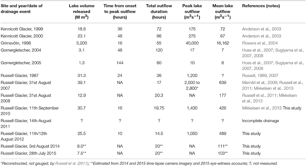
Table 1. Metrics for events where both transient lake level measurements have been obtained and also to where lake bathymetry is known, together permitting lake outflow (discharge) to be calculated.

Study Site and Measurements

A ~1 km² ice-dammed lake on the northern flank of Russell Glacier, west Greenland (Figure 1) is known to have drained repeatedly from the late 1940s until 1987 (Sugden et al., 1985; Russell and de Jong, 1988; Russell, 1989). Following 20 years of relatively stable lake level, a jökulhlaup on August 31st 2007 marked renewed ice-dammed lake drainage (Mernild et al., 2008; Mernild and Hasholt, 2009) and a new jökulhlaup cycle (Russell et al., 2011). To date, this new cycle has resulted in floods almost every year (Table 1). This lake has a history of being studied for its lake drainage mechanism(s) (e.g., Russell and de Jong, 1988; Scholz et al., 1988; Russell et al., 2011).

FIGURE 1

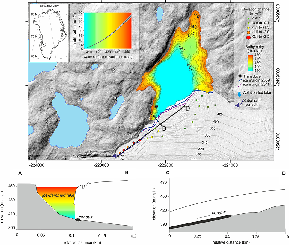
Figure 1. Study site location, topography and detail of conduit geometry. Circles denote rates of change in elevation as calculated between August 2011 DEM and field surveyed points in May 2015. Profiles of ice surface and subglacial bed elevation are depicted along transects (A,B) and transects (C,D), as indicated on map. Contours on ice are bed elevation. Map grid coordinates are UTM 22N.

Ice surface elevations were surveyed in the field in 2010 and 2015 using a Leica GPS500. We used a temporary base station, positioned relative to the Kellyville International Geodetic System network continuous receiver, via post-processing of a 10-h static occupation and recording at 1 min intervals, and with a vertical precision of ± 0.01 m. From this temporary base station our rover points, or points of interest on the ice surface (Figure 1), which were obtained in real time static mode (using the geometric mean of 120 static readings), have a vertical precision of ± 0.15 m.

Further distributed ice surface data were gained from a 2 m digital elevation model (DEM) that was produced by photogrammetric processing of stereo-pairs of DigitalGlobe imagery, specifically via the Surface Extraction with Triangulated Network-based Search-space Minimization (SETSM) algorithms (Noh and Howat, 2015). Note that whilst denoted as from year 2011, this is a composite DEM, the seamless coverage being constructed from multiple image pairs from multiple flight lines from multiple dates. In order to consider any relationship between change in lake level and change in ice dam thickness, elevation differences between our 2015 dGPS field surveys and the 2011 DEM have been converted to annual rates of change in surface elevation and these show surface lowering in the vicinity of the subglacial conduit that is more than double that across the rest of the ice margin (Figure 1).

Glacier bed topography, indicated by contour lines in Figure 1, was obtained by combining 1 km resolution ice thickness data (Bamber et al., 2013), a regional InSAR-derived ice surface (Palmer et al., 2011) and local IceBridge flightline data (Leuschen et al., 2017) and was gridded at 0.1 km cell size. This bed topography shows that the Russell Glacier margin abuts the ice-dammed lake on an adverse gradient bed slope (Figure 1). Recognition of the fact that the glacier bed is inclined downwards in a cross-flow direction is important for understanding ice margin dynamics, the configuration and evolution of the subglacial drainage network and subglacial water pressure, all of which we refer to later.

A seamless digital elevation model was constructed by combining the 0.1 km interval subglacial bed contours with the 5 m proglacial terrain elevation contours and interpolating the remaining ice-dammed lake floor using the ANUDEM algorithm, which is within the ArcGIS “Topo to Raster” tool. This seamless digital elevation model enabled us to make spatially distributed calculations of hydrostatic pressure and ice overburden pressure for scenarios of varying water depths and varying ice surfaces or ice thickness.

The ice-dammed lake drains (almost every year; Table 1) via a subglacial conduit with stable inlet and exit positions (Figure 1). From these positions, we derived an approximate straight planform length of 650 m and a conduit gradient of ~0.015 m m⁻¹ (Figure 1). The hydraulic gradient of this conduit is low, due to the relatively shallow ice surface and bed topography slopes (Figure 1). Field observations and photographs of the conduit inlet and exit portals show that the conduit is elliptical in cross-section and has a diameter (at both inlet and exit portals) of ~ 5 m vertically and ~ 15 m horizontally; direct measurements have never been possible because both portals are unsafe to access. Lake basin bathymetry (Figure 1) is well-known from differential Global Positioning System (dGPS) surveys conducted when the lake basin was almost completely drained (Russell et al., 2011).

In anticipation of ice-dammed lake drainage, a HOBO U20 pressure transducer, with range from 0 to 76.5 m and an accuracy of ± 0.05%, was installed in mid-May 2010 (as indicated in Figure 1) when the lake level was at 432.5 m a.s.l., which is 27.5 m above the conduit inlet portal. The transducer was weighted to ensure it remained on the lake bed. The HOBO recorded average lake water pressure and lake water temperature at 15 min intervals. Lake drainage events were recorded by the pressure transducer on 11th September 2010, 11th August 2012, by time-lapse cameras on 3rd August 2014, and by the same cameras accompanied by dGPS measurements on the 28th July 2015. The 2010 and 2012 lake water pressure records were corrected for atmospheric air pressure recorded 2 km away from the ice-dammed lake with an automatic weather station (AWS) using Campbell Scientific sensors operating continuously year-round. The AWS data showed that seasonal weather up to and including the drainage events was not unusual, thereby assisting in ruling out any external trigger to the drainage events. A simple calculation of the melt season up to the day of lake drainage, made with the AWS data, gives 116, 75, 46, and 60 positive degree days for 2010, 2012, 2014, and 2015, respectively.

In 2010, the ice-dammed lake filled by 1.1 ± 0.1 × 10⁷ m³ over 112 days from mid-May to early September (Figure 2A), equating to an average inflow rate of 1.14 m³ s⁻¹. This inflow rate is very similar to Russell et al.'s (2011) estimate of 0.6 to 1.3 m³ s⁻¹, which was derived from supraglacial stream gauging only. Calculations performed on the 2012 lake level data suggest a lake refill rate of 2.4 m³ s⁻¹, but in contrast only 0.86 m³ s⁻¹ in 2014 and 0.87 m³ s⁻¹ in 2015. The 2012 refill rate is presumably high because of the extreme ice surface melt experienced over the Greenland Ice Sheet (GrIS) (Nghiem et al., 2012) during this year. Comparison between these lake refill rates and stream inflow rates demonstrates that there are no substantial subglacial inflows to the ice-dammed lake, that subglacial leakage from the ice-dammed lake during lake filling is negligible, and thus that the seasonal and event water balance(s) can be considered simple and closed.

FIGURE 2

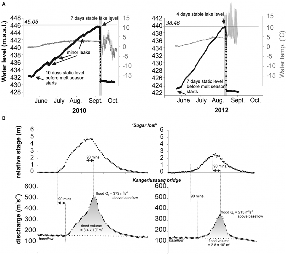
Figure 2. Lake water level and water temperature record for ablation seasons 2010 and 2012 (A). The gray shaded bars denote the time period depicted in Figures 4A,B. Italicized numbers refer to the maximum thickness of ice that could be liable to flotation given the water level and thus water depth and hydrostatic pressure in comparison to ice overburden pressure. Note varying y axis scales. Panel (B) depicts gauged hydrographs ~ 23 km downstream at “Sugarloaf” and ~ 32 km downstream at Kangerlussuaq bridge, both after data by Hasholt et al. (2013) and Mikkelsen et al. (2013).

These refill rates and our interpretations of water inflows to the ice-dammed lake are important because the few previous studies that have obtained direct measurements of ice-dammed lake drainage have found it necessary to deal with complications in the event water balance. These complications have primarily been: (i) significant upstream inputs to the lake (e.g., at Kennicott Glacier: Anderson et al. (2003); at Grímsvötn: Flowers et al. (2004); at Merzbacher lake where Ng et al. (2007) reconstruct inflows of up to 100 m³ s⁻¹ during flood discharges typically of 1,000 m³ s⁻¹), and (ii) release of significant volumes of water from storage within the glacier over and above that draining from the lake; e.g., Huss et al.'s (2007) calculations imply that up to 40% of a jökulhlaup from Gornersee came from non-lake water within Gornergletscher. In comparison, the Russell Glacier ice-dammed lake drainage events have a mean rate of water release that is up to two orders of magnitude greater than other (non-volcanically triggered) measured sudden lake level falls (Table 1). Indeed the 2010 and 2012 events at Russell Glacier had mean outflows of 426 m³ s⁻¹ and 489 m³ s⁻¹, respectively (Table 1), which is equivalent to ~10 and ~11 Olympic swimming pools draining per minute, respectively. These mean outflows exceed the normal summer ice melt discharge observed (but not gauged) through the exit portal by two orders of magnitude. They also have a relatively simple water balance; (i) subglacial water inputs to the ice-dammed lake throughout the summer were negligible as evidenced by lake refill rates that agree well with gauged supraglacial meltwater runoff, as described above, and (ii) inflow to the lake was volumetrically negligible during the lake drainage events since both events lasted just hours rather than days.

Determination of Lake Outflow Hydrographs

In both 2010 and 2012, the ice-dammed lake water level drained below the elevation of the pressure transducer, as indicated mainly by the sensor temperature record. In order to constrain the later part of the rising limb, it was therefore necessary to reconstruct the peak and falling limb of the outflow hydrograph for both the 2010 and 2012 ice-dammed lake drainage events. Hydrograph reconstruction (Figure 3A) assumed that the rate of change in lake level drawdown (Figure 3B) increased linearly until a time t₁, and then decreased linearly to zero at time t₂, these assumptions being motivated by the roughly symmetrical shape of the hydrographs measured downstream (Figure 2B). t₂ was chosen from the period of the flood gauged downstream of 11 and 20 h for the 2010 and 2012 events, respectively (Hasholt et al., 2013; Mikkelsen et al., 2013). t₁ was chosen such that the total volume drained (Figure 3C) within the time interval was consistent with that gauged downstream (Figure 2B). We acknowledge that flood hydrograph durations typically lengthen with distance down-conduit and down-stream (e.g., Evans and Clague, 1994; Carrivick et al., 2013) so our flood duration is likely to be an over-estimate. Given the assumptions and uncertainty associated with reconstructing the flood recession phase, we will not use the falling limb to constrain our subsequent numerical modeling of the discharge evolution. However, we were motivated to reconstruct the lake water level draw-down in order to (i) estimate a final (post-drainage) lake level and a lake outflow hydrograph (Figure 4A), and (ii) for comparison with other events at Russell Glacier and elsewhere (Table 1).

FIGURE 3

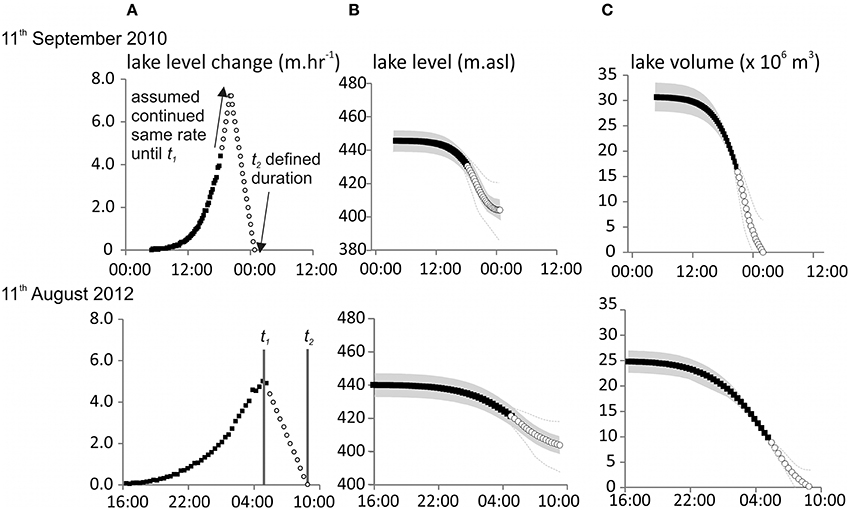
Figure 3. Measured lake outflow (black filled squares) with reconstruction (gray filled circles) of the latter part of each event using rate of change of lake level (A), absolute lake level (B) and lake volume (C). Gray shaded areas are indicative of uncertainty range due to pressure transducer and dashed lines indicate uncertainty range due to reconstructions using downstream gauged data.

FIGURE 4

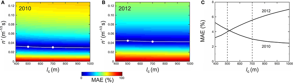
Figure 4. (A,B) Mean absolute error (MAE) of the misfit between simulated and observed hydrographs for 2010 and 2012 for different values of Manning roughness n' and conduit length l_c, plotted in color over their parameter space. White lines locate minimum MAE for each l_c. Dots locate the model runs in Figure 5 for l_c = 700 m and l_c = 500 m. (C) Minimum MAE as a function of l_c for the two outbursts.

In 2014 our pressure transducer was inoperable after mid-July and in autumn 2015 it could not be recovered due to becoming struck by rockfall, so we cannot constrain the rate of change of outflow in 2014 and 2015. Whilst we could constrain the conduit inlet elevation and the lake volume change in 2014 and 2015 via time-lapse imagery and via dGPS measurements, these together indicated lower volumes and slower rates of outflow than in 2010 and 2012 and so, without the ability to evaluate any numerical model output, we do not consider these later two events further in this paper.

Overall, the uncertainty in our pressure-level measurements due to sensor resolution and precision is ± 0.05%. Uncertainty in the SETSM DEM elevations for the flight strip used in this study is a maximum of 4 m (Noh and Howat, 2015). Uncertainty in our subglacial bed elevation interpolations and thus ice thickness calculations (Figure 1) is of the order of 20% as a function of the radio echo sounding data collection, interpolation between transects and combination of these data with subaerial topography. Uncertainty in our lake bathymetry interpolations is likely to be ±5%. Given these uncertainties, and the propagation of them (through multiplication of area by elevation change to get volume, and through differencing of DEMs, for example), our field measurements for 11th September 2010 determined a flood volume of 3.1 ± 0.3 × 10⁷ m³. We assumed that the flood hydrographs were near-symmetrical and our reconstructions yielded a peak discharge of 1,430 ± 150 m³ s⁻¹ for the 2010 event. For 11th August 2012 we measured a flood volume of 26 ± 0.3 × 10⁷ m³ and reconstructed a peak discharge of 1,050 ± 140 m³ s⁻¹.

Lake Outflow Model

Model Equations

We model how discharge Q evolves in each flood using a simplified Nye (1976) model of a subglacial conduit (of length l_c, cross-sectional area S) draining the lake. The model is “lumped”—it assumes a “short” subglacial conduit and neglects spatial variations, so variables are functions of time t only (cf. Ng, 1998; Bueler, 2014). This approximation holds because l_c ≲ 1 km and the hydraulic gradient (Ψ) is sufficiently low so that meltwater from the conduit walls contributes negligibly toward Q, as is confirmed by the small parameter ε = Ψ l_c/ρ_iL ≈ 10⁻³ (Ng, 1998; Fowler, 1999; Ng and Björnsson, 2003) in a formal scaling analysis of our system. Although ε does not account for extra melting along the conduit induced by lake thermal energy, our simulation of the flood events later show that this additional melt source is small and does not invalidate the approximation. Specifically we solve the differential equations:

$\begin{array}{ll}\frac{\text{d}S}{\text{d}t}=\frac{m}{{\rho }_i}-K_{0}S{N}^n& (1)\end{array}$

$\begin{array}{ll}\frac{\text{d}V}{\text{d}t}=Q_{\mathrm{\text{IN}}}-Q& (2)\end{array}$

for the coupled evolution of conduit size S and lake volume V. Equation (1) expresses the competition between conduit enlargement due to wall melting (which occurs at the rate m) and viscous closure at a rate dependent on effective pressure N = ρ_igH – p_w, where H is ice-dam thickness next to the lake (55 m), and p_w is the conduit water pressure, which is determined by the hydrostatic lake pressure at the conduit inlet; accordingly, p_w = ρ_wgh, where h is the lake water depth. As the lake drains, h decreases, raising the effective pressure N and enhancing closure. In Equation (2), Q_IN denotes the rate of water inflow feeding the lake, which derives from snowmelt and precipitation in the subaerial catchment and any subglacial contribution (or leakage). The standard physical constants in this model are given in Table 2. The closure rate constant K₀ in Equation (1) is based on the creep rate of ice at 0°C because we assume this part of Russell Glacier to be temperate. Temperature measurements are lacking, but our simulations below show that the closure term is entirely negligible, so cold ice (yielding smaller K₀) will make no difference.

TABLE 2

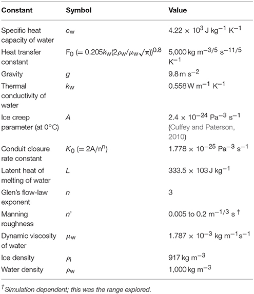
Table 2. Phenomenological constants in our model.

At any time during flood evolution, we find the lake water depth h from the lake volume V by inverting the lake bathymetry shape function known from field measurements made by Russell et al. (2011):

$\begin{array}{ll}V=8.014\times {10}^{-3}{z}_L^2-6.048z_L+1134.5& (3)\end{array}$

where V is in 10⁶ m³, z_L = h + z_LB is the lake surface elevation (m) and z_LB = 405 m is the conduit inlet elevation above sea level. Following Nye (1976), the instantaneous discharge is calculated using the Manning Equation for momentum conservation in turbulent water flow:

$\begin{array}{ll}Q=\sqrt{\frac{\text{Ψ}}{F_1}}{S}^{4/3}& (4)\end{array}$

in which the constant F₁ encapsulates the Manning roughness n' and cross-sectional shape of the conduit (see definition by Nye (1976), who symbolized it with a calligraphic-N). Since our field observations show that the conduit lies at the ice-bed interface at its two ends (at the lake and glacier snout), we assume a semi-circular cross section for it; then F₁ = (2(π+2)/π)^2/3ρ_wgn'². In Equation (4), Ψ is the spatial mean hydraulic gradient driving the flow:

$\begin{array}{ll}\text{Ψ}={\text{Ψ}}_g+\frac{N_{exit}-N}{l_c}.& (5)\end{array}$

Ψ_g is the glaciostatic gradient = 537 Pa m⁻¹ from topographic data, and the fraction measures the effective pressure gradient along the conduit, which is time-varying because the lake water depth controls N, as mentioned earlier. We expect the flow to transition from closed-conduit (pressurized) to open-channel (atmospheric) some distance back from the exit portal, because thinner ice and the local stress distribution at the snout cause creep closure to become negligible there (Evatt, 2015). N_exit is the effective pressure at this transition, and our definition of l_c strictly refers to the length of closed-conduit flow. Neither quantity is observationally well-constrained. In our modeling we specify N_exit = ρ_ig × 35 m, where 35 m (the ice thickness at the transition) is taken from the regional ice thickness near the snout (Figure 1C). To cater for uncertainty in both this assumption and the conduit's trajectory, we conduct sensitivity analysis in our simulations by varying l_c from the estimated curvilinear path distance between the lake and the exit portal (700 m); e.g., l_c would be higher for a more sinuous conduit, or less if open-channel flow is more extended. [Additional sensitivity analysis on N_exit or the threshold thickness is possible, but not especially insightful, because changes in these can be absorbed into changes in l_c; see Equation (5)].

The use of spatial mean gradients is consistent with our “short conduit” approximation and convenient because the subglacial flood path at Russell Glacier is only approximately located. Nye (1976) and Clarke (1982) also assumed mean hydraulic gradients when applying their models, but neglected the effective pressure gradient (the fraction) from Equation (5). At Russell Glacier, the lake's proximity to the exit portal and high ratio (~1) of its water depth to the elevation drop along the conduit means that the effective pressure gradient strongly controls Ψ when the lake level falls during an outburst. As we shall see, this effect can cause the simulated flood discharge to reach its peak and fall shortly before the lake runs empty.

Finally, we calculate m in Equation (1), which is the mean melt rate along the conduit in our lumped model. We do this by using a formula from Ng et al. [2007; Equations (A3) and (A4)]:

$\begin{array}{ll}mL=(1-\alpha )Q\text{Ψ}+\alpha F_0{\left(\frac{\text{Ψ}}{F_1}\right)}^{3/20}{Q}^{1/2}{T}_L,& (6)\end{array}$

where T_L denotes the lake water temperature. This formula encapsulates energy conservation and turbulent heat transfer and is based on the pseudo-steady profile of the water temperature along the conduit, which equilibrates on a much faster timescale than flood evolution. Its derivation from Nye's (1976) original model is detailed in the Supplementary Information (SI), where we explain why it captures the heat-transfer mechanisms appropriately, and discuss a concern raised by Clarke (2003) about other formulas for m used in jökulhlaup lumped models. Appearing twice on the right-hand side of Equation (6), the thermal partitioning coefficient α (between 0 and 1)

$\begin{array}{ll}\alpha =\frac{1-e^{-\beta }}{\beta }\text{ where }\beta =\frac{F_0{l}_c}{{\rho }_w{c}_w\sqrt{Q}}{\left(\frac{\text{Ψ}}{F_1}\right)}^{3/20}& (7)\end{array}$

accounts for downstream heat advection, heat transfer between water and conduit wall, and dissipation of potential energy in warming the flow, all of which depend on the changing discharge. As shown in the SI, the instantaneous temperature profile along the conduit is the sum of two temperature distributions: (i) a growing exponential [∝ 1−exp(−βx/l_c)] due to potential energy dissipation at rate QΨ along the conduit, and (ii) a decaying exponential [∝ exp(−βx/l_c)] due to water entering the conduit at temperature T_L and losing its heat to the walls. The dimensionless parameter β governs the growth/decay rate of these exponentials, and α is the spatial mean value of exp(−βx/l_c) over the conduit. The relationships in Equation (7) show that β ∝ l_c/√Q, and that α is a decreasing function of β such that at the limits β → 0 (a “thermally short” conduit) and β → ∞ (a “thermally long” conduit), α = 1 and α = 0, respectively. Correspondingly, on the right-hand side of Equation (6) are two separate contributions to m from potential head loss (first term) and lake thermal energy (second term). In the first term, a fraction α of QΨ does not cause melting as it has been used to warm the conduit flow. In our simulations, we assess the relative sizes of these terms during each flood event.

Flood Simulation: Set Up

Equations (1) and (2) are integrated numerically forward in time by explicit finite-difference (Euler) method until h = 0. As the model neglects the flood-initiation process (e.g., Fowler, 1999; Kingslake and Ng, 2013), we specify initial conditions for S and V at a time after flood initiation. A novelty of this study is that these are known coincidently from the “highstand” lake depth h_HS in our recorded lake-level histories (Figure 2A). Highstand marks the point after flood initiation when Q is still small but has grown to balance Q_IN momentarily (Ng et al., 2007); its timing is not easy to pinpoint due to fluctuations in Q_IN and pressure-transducer noise. However, h_HS yields accurate initial conditions for V(t = 0) via Equation (3) and S(t = 0) via Equations (4) and (5) (where we set Q = Q_IN and N = ρ_igH − ρ_wgh_HS). Table 3 lists h_HS for the two outburst floods. Without lake-level monitoring data, other ways of constraining the initial conditions would be necessary, e.g., using the observed flood volume together with observed flood peak discharge, as discussed by Ng et al. (2007).

TABLE 3

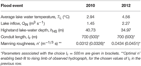
Table 3. Parameters used in flood hydrograph simulations.

We prescribe Q_IN as the mean rate of lake-volume rise over the preceding 2 months (Table 3). We set T_L to the mean value of the measured lake-water temperature during each flood, which varied by 0.5°C in 2010 (between 2.7 and 3.2°C) and by 0.7°C in 2012 (between 4.2 and 4.9°C). Although we did not measure vertical temperature profiles in the lake, the limited (and smooth) variations suggest the lake water to be relatively well-mixed, not strongly stratified. In our model runs, we therefore assume that water temperature measured by the pressure transducer is representative of the water temperature at the inlet portal. Its temporal mean is adopted because the measured variations could be due to circulating lake water with spatially-non-uniform temperature, in which case their size (up to ±0.35°C) would indicate the potential error of using the temperature at the transducer as the inlet temperature. While we lack observations to support/refute this assumption, sensitivity analysis later (Figure 6A) shows that such error would alter the simulated peak discharge by several hundred m³ s⁻¹ if other parameters are held constant.

Results and Analysis

Numerical runs are made with different combinations of Manning roughness n' and (closed) conduit length l_c to simulate each year's hydrograph for comparison with the observed hydrograph. Since the equations are autonomous and the lake highstand too loosely located in time for us to put the “t = 0” precisely on the observational time line, in each comparison we always first align the hydrographs in time by sliding the simulated one against the observed one until the Mean Absolute Error (MAE) in Q between them is minimized for their overlap period. The MAE is then reported as a percentage of the mean observed discharge for the period. This procedure uses only measured discharge data on the rising limb and ignores reconstructed data (as these are more uncertain), so it is not aimed at fitting the flood peak.

For both 2010 and 2012, the map of MAE across the parameter space of n' vs. l_c (Figures 4A,B) implies a weak influence of conduit length on the success of fit. MAEs <10% are found along the valley axes (Figure 4C). Within a plausible range of l_c (400 to 1000 m), neither map shows a minimum point in MAE that identifies the best combination of n' and l_c. The weak influence of l_c found here means that it cannot be constrained based on the fit on the rising limb alone.

For each choice of conduit length, the minimum MAE identifies an optimal n' allowing best fit of the rising limb of the hydrograph (white curves in Figures 4A,B); we call the corresponding numerical run an “optimal simulation”—for that l_c. For the l_c range studied here, optimal values of n', ≈ 0.03 to 0.045 m^−1/3 s, fall within the range encountered in jökulhlaup studies [~0.01 to ~0.1 m^−1/3 s Ng, 1998; Fowler, 1999; Clarke, 2003; Werder and Funk, 2009; Kingslake, 2013]. Figure 5 shows the modeled lake level and outflow hydrograph histories in the optimal simulations for l_c = 700 m, and Table 3 lists the corresponding n'. The simulated lake levels match the observed histories well for most of the flood duration (Figures 5A,B). In both years, the model captures the shape of observed discharge on the rising limb successfully (MAE = 3.0% in 2010 and = 5.6% in 2012). The simulated peaks occur slightly later than expected from our reconstructions and overshoot the reconstructed peak discharge by 100 to 200 m³ s⁻¹. For both years, these matches to the reconstructed peak discharge are improved if we assume a shorter section of closed-conduit flow, e.g., l_c = 500 m (blue curves, Figures 5C,D). Then the simulated peaks are lowered to near the reconstructed peaks, while the MAEs for the rising limb remain acceptable (4.3% in 2010 and 4.0% in 2012, Figure 4C). These findings suggest that there might have been a considerable (≈ 200 m long) section of open-channel flow behind the exit portal in both the 2010 and 2012 events; however, we emphasize that this inference is very tentative because our peak discharge values are reconstructed, with large uncertainties of ±140 to 150 m³ s⁻¹. On the other hand, this exercise of varying l_c shows that a matching procedure that best-fits the peak discharge as well as the rising limb can constrain l_c as well as n'—at least for the parameter region studied here. An accurate and complete measured hydrograph would be needed for this purpose. Note that the choices of l_c in these experiments are illustrative: we are not implying that l_c is the same in different floods. However, our modeling assumes l_c to be constant in each simulation/flood, and this may not be an accurate description.

FIGURE 5

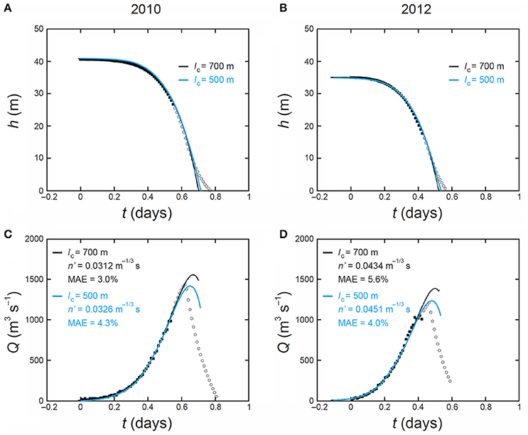
Figure 5. Best-fit simulated lake level histories (A,B) and flood hydrographs (C,D) for the 2010 and 2012 outbursts when l_c = 700 m (black curves) and l_c = 500 m (blue). Solid squares show measured data and gray circles reconstructed data. In all panels, the time axis t places the first measured data point used in the hydrograph-fitting exercise at t = 0. In (C,D), the mean absolute error (MAE) of misfit between model and measured data and the optimal Manning roughness n' are indicated.

The modeled floods terminate with Q falling to zero abruptly, in a manner noted by Clarke (2003), when the lake level falls below the conduit inlet elevation (Figure 5). While this describes the situation at the lake, remaining water in the conduit takes time to evacuate, and an expansion wave causes Q at the exit portal to decrease more gradually (Fowler and Ng, 1996). For each year, the flood volume released by the lake is nearly invariant across our simulations because the model uses the same initial lake level (h_HS), and the cumulative inflow into the lake (which is drained in the flood) is very small. The flood volume at the exit portal is slightly higher due to the added conduit meltwater, but only by ≈ 0.2%, so the short-conduit approximation used in the model is self-consistent.

Our sensitivity experiments reveal an acute influence of lake water temperature on the flood hydrograph (Figure 6A), which is stronger than that of other factors within their conceivable range of variations (Figures 6B–E). The same qualitative finding was reported by Werder et al. (2010) in their modeling study of a supraglacial lake that drained through englacial/subglacial pathways. Warming the lake by a couple of degrees Celsius raises the peak discharge and shortens the flood substantially, whereas T_L near 0°C stretches the hydrograph to a much lower peak over a week or more (Figure 6A). This contrast is similar to that between volcanically-triggered (rapidly-rising) jökulhlaups and the more common (slower-rising) jökulhlaups from Grímsvötn (Björnsson, 2002; Roberts, 2005). We conclude that T_L of several degrees Celsius, coupled with the short ice dam, are the most major factors controlling the peak magnitude, the timing of peak magnitude, and the short flood durations (<1 day) in 2010 and 2012. These same factors are likely responsible for similar outburst characteristics in other years at Russell Glacier (Table 1).

FIGURE 6

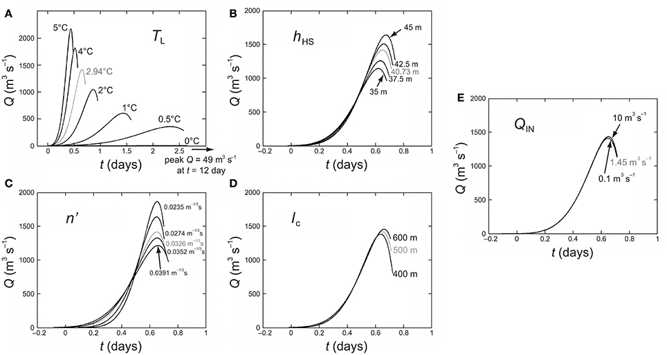
Figure 6. Numerical sensitivity experiments showing the effect of altering individual parameters on the 2010 flood hydrograph, using the optimal model run for l_c = 500 m as control. Parameters are: (A) Lake water temperature T_L; (B) highstand lake level h_HS; (C) Manning roughness n'; (D) conduit length l_c; (E) lake inflow rate Q_IN. Results for l_c = 700 m and for 2012 are qualitatively similar.

The sensitivity results in Figures 6B–E provide additional insights for the simulation of the Russell-Glacier floods in the contexts of hydrograph matching and prediction. The simulated hydrograph is largely insensitive to the lake inflow rate Q_IN (Figure 6E), so our using a Q_IN-estimate from the months before each flood to approximate Q_IN during the flood is reasonable. This approximation may serve well in other purely predictive runs, although dedicated sensitivity tests should be performed in each case. The peak region of the simulated hydrograph is sensitive to the highstand lake depth h_HS (Figure 6B), with the peak discharge varying by roughly ±50 m³ s⁻¹ per meter error in h_HS (a similar result is found in 2012 and 2010, for both l_c = 500 and 700 m). Thus, lake-level monitoring to determine h_HS with sub-meter accuracy is necessary for the model to match/predict the flood peak correctly to within this uncertainty range—our pressure transducer easily meets this requirement. The results for l_c and n' (Figures 6C,D) inform the question of constraining these parameters through matching the observed flood hydrograph, which we encountered earlier. Whereas the peak of the simulated hydrograph and the curved shape of its rising limb are both sensitive to n', only the peak is sensitive to l_c. This finding explains why the MAE of fit on the rising limb depends weakly on l_c (Figure 4), why the procedure of minimizing this particular measure of error constrains n' but not l_c, and why matching the peak discharge also (if this is known reliably) should constrain l_c as well as n'. These interpretations from Figure 6 are based around a specific set of model parameters; model sensitivity far from this region of the parameter space may be very different.

Discussion

Our numerical simulations yield new insights into the thermomechanical characteristics of the 2010 and 2012 floods. When these insights are considered with the information from our other datasets, we are able to consider the entirety of each sudden drainage event, not just the rising limb, and also the most likely trigger of drainage.

Thermomechanical Contributions

Throughout each simulation in Figure 5, melt enlargement dominates conduit evolution, with viscous closure being negligible in comparison. Indeed, we find that removing or doubling the closure term in Equation (1) merely changes the simulated peak discharges by ≈1 m³ s⁻¹. This is partly due to low overburden pressure from a thin ice dam, and partly because other factors precondition an intense melt rate, as will be discussed next. Consequently, the simulated turnaround of discharge at the flood peaks is not caused by closure overtaking melting, but by rapidly decreasing potential energy and hydraulic gradient as the lake depth h falls toward zero. In our model, including the effective pressure gradient (the final fraction) in Equation (5) is crucial for capturing this behavior at Russell Glacier. Accordingly, our simulations show that the conduit continues to enlarge at the times of peak discharge (Figures 7A,B) while the hydraulic gradient causes the melt rate to reach a maximum and then decrease (Figures 7C,D).

FIGURE 7

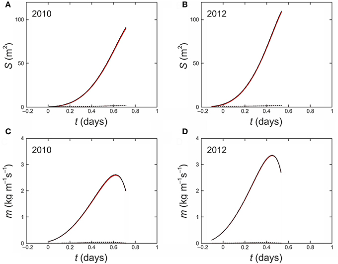
Figure 7. Modeled histories of conduit cross-sectional area S (A,B) and melt rate m (C,D) in the simulations for l_c = 500 m in Figure 5. (Qualitative results for l_c = 700 m are similar). In individual panels the black curve plots S or m; the red curve plots the component (of S or m) due to lake water temperature and the dashed curve the component due to hydraulic head loss.

In contrast, Nye (1976) envisaged for the 1972 jökulhlaup from Grímsvötn that sudden dominance of an accelerating viscous closure rate over melt rate (in Equation 1) is what caused flood discharge to attain its peak value in that system. We do not think that this difference in behavior between Russell Glacier and Grímsvötn indicates fundamentally different flood-thermomechanical processes in operation in these systems, or that any process has been overlooked or misinterpreted in either system. Instead, it reflects different relative magnitudes of melting and closure. Notably, much greater thickness of the ice dam at Grímsvötn (≈220 m) implies that creep closure exerts a stronger influence on flood evolution of a comparable size to that of melting. On the other hand, the much smaller surface area of the lake at Russell Glacier facilitates its rapid lowering (toward emptying) such that a short flood duration limits the time over which closure reduces the conduit cross-section. Our results here thus highlight the importance of local site factors in GLOF dynamics. Through mathematical analysis of the ratio of the closure timescale to the flood-duration timescale for jökulhlaup systems generally, it should be possible to explain what delineates the two types of behavior (Ng and Björnsson (2003) explored an early theory, neglecting lake thermal energy, for lakes whose depth is a small fraction of the conduit elevation drop).

The finding that melt enlargement dominates outburst flood evolution at Russell Glacier prompts us to examine the contributions to m and S, and this leads us to appreciate how strongly lake water temperature (T_L) determines the floods' size and duration, and the role of a short subglacial conduit in this effect. Equation (6) identifies (i) energy dissipation from potential head loss in the flow (QΨ) and (ii) lake thermal energy as the two contributions; these contributions have independent additive effects on conduit wall melting, through their influences on water temperature (see Supplementary Information). Figure 7 shows that the contribution to melt enlargement is dominated by lake water temperature. The reasons for this are two-fold. Firstly, the maximum possible warming of the water from potential head loss, g[h_HS + Δz]/c_w = 0.15°C, is itself an order of magnitude smaller than T_L in both floods (several degrees Celsius; Table 2). The actual warming experienced by the water (when it reaches the exit portal) is still less than the maximum possible, because the conduit is “thermally short,” so the temperature addition from “QΨ” (contribution i) is still increasing spatially toward the maximum. This is reflected by a high value of α (≳ 0.6) throughout flood evolution (Figure 8), and the attendant low value of (1 −α) multiplying into QΨ in Equation (6). Secondly, the same factor makes the lake-thermal contribution (contribution ii) efficient because the conduit is short and thus the water temperature has not decreased much from T_L by the time it reaches the exit portal. Hence the mean temperature driving heat transfer behind melting along the conduit is high (a large fraction of T_L), and this is reflected by the high α-value in the last term of Equation (6). Despite the resultant high heat transfer, there is a limited decay in water temperature along the conduit because of the short transit time of the flow. In these evaluations, it is important that Equation (6) captures the conduit heat transfer appropriately. This is shown to be the case in the SI, where we also discuss Equation (6) alongside other heat-transfer formulas that had been critiqued by Clarke (2003).

FIGURE 8

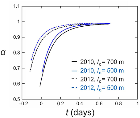
Figure 8. Variation of the thermal partitioning coefficient α in the four model runs for the 2010 and 2012 outbursts in Figure 5, with l_c = 700 m (black curves) and l_c = 500 m (blue curves).

As noted before, we have observed that the inlet and exit portals of the conduit are elliptical and with 5 and 15 m vertical and horizontal width dimensions, respectively. The outlet portal survives from one season to the next with “normal” ice meltwater discharge. It seems unlikely that a channel at the ice margin that had grown to 100 m², as suggested by our modeling, would completely collapse between each field season. This is because the ice is thin and whilst we have looked (and surveyed with dGPS) there is no evidence that a large channel was formed, or that one collapsed, such as surface depressions on the ice surface. Nonetheless, whilst some (lateral) advection of the conduit probably occurs between floods, due to ice motion northwards, we suppose that the conduit is surviving from one season to the next. Indeed, in the field we observe “normal” meltwater exiting the outlet portal throughout each spring-summer-autumn season. We therefore consider it likely that the conduit seals between floods only in the vicinity of the inlet portal.

One challenge is that at Russell Glacier, and indeed most likely at many other sites of ice-marginal lake drainage, segments of conduits that are at atmospheric pressure for some distance up-glacier from the conduit exit portal are best represented by conditions of open conduit flow. Whilst Nye (1976) did not assume that the conduit was all at ice overburden pressure in his model; i.e., that the effective pressure N = 0, he did assume that dN/dx = 0, where x is the along-conduit dimension. That assumption does not hold for drainages of most ice-marginal lakes where ice dam thickness is just a few tens of meters.

Interpretation of Flood Trigger and Influence on Drainage Evolution

Analysis of ice thickness, bed topography, lake bathymetry and knowledge of lake levels demonstrates that the threshold for ice-dam flotation being reached was possible and indeed very likely. Specifically, flotation can occur if hydrostatic pressure, ρ_wgh, where h is water depth as calculated by maximum water level minus the elevation of the conduit inlet, exceeds ice overburden pressure, ρ_igH where H is ice thickness (e.g., Sturm and Benson, 1985; Tweed, 2000). With the conduit inlet at 404.5 m a.s.l. and given water depth evolution through the ablation season (Figure 2), hydrostatic pressure would have been reached if the glacier ice-dam was ≤45.05 m thick in 2010 and ≤38.46 m thick in 2012. This means that the ice in the vicinity of the conduit inlet had the capability to float in both 2010 and 2012 (Figure 9). Quantifiably, if the lake water surface elevation reached 440 m, as in the year 2012, then lake water depth at the conduit inlet would exceed 27 m and ice with thickness of <30 m, as colored in Figure 9, would be susceptible to flotation.

FIGURE 9

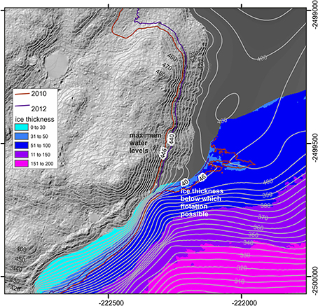
Figure 9. Detail of the vicinity of the subglacial conduit, with interpolated contours at 5 m intervals, and ice thickness calculated as the difference between the bed and the ice surface in a DEM derived from August 2011 stereo images. Maximum water levels are marked in years 2010 and 2012 and the corresponding ice thickness below which flotation would be possible is delimited. Map grid coordinates are UTM 22N.

Our conceptual model for the entirety of both drainage events therefore hypothesizes flotation as the trigger (Figure 10). Notwithstanding our spatial analysis of ice overburden pressure vs. hydraulic head, this hypothesis requires further investigation. We suggest that the two floods were triggered with the lake level lower in 2012 compared to 2010 because the ice-dam had thinned, for which there is evidence from oblique field photographs, eye-witness reports from the Greenlandic mountain guide Adam Lyberth [pers. comm.], and comparison in this study of ice surface elevation made via ground-based dGPS surveys in 2015 and from a digital elevation model constructed from stereo images acquired in 2011.

FIGURE 10

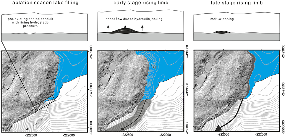
Figure 10. Schematic to illustrate evolution of ice-dammed lake water level and subglacial conduit to explain lake drainage mechanisms. Arrows denote likely subglacial conduit pathway. Contours denote bed elevation.

Hydraulic jacking due to lake water pressure/head in the vicinity of the conduit, simultaneous with thermal erosion, could have facilitated extremely rapid water egress during the first third of the rising limb of each flood (Figure 10). This contribution of hydraulic jacking might explain the particularly rapid (very high mean outflow rate) water egress at Russell Glacier, in comparison to that recorded for other ice-marginal lakes (Table 1). Thus, rather than a model of a single R-channel, a coupled sheet-conduit model such as that of Flowers et al. (2004) could be more appropriate, as has recently been applied by Einarsson et al. (2017) to a rapidly-rising jökulhlaup in Iceland.

As lake water level fell, ice overburden pressure caused remaining outflow to be progressively confined to the conduit. Thereupon melt enlargement became the dominant mechanism permitting discharge increase up to peak outflow (Figures 5C,D, 10). The sharply-inclined falling limb was produced as a function of the low hydraulic gradient, which itself was a function of the high ratio (~1) of change in lake water depth to the elevation drop along the conduit.

Conclusions

Understanding the controls on the timing, magnitude and thermomechanical dynamics of GLOFs is complex. This study reports a rare set of comprehensive field measurements from an ice-dammed lake in west Greenland and has used them to evaluate the likely lake drainage trigger and to quantitatively assess the mechanisms of drainage evolution.

Following hypothesized flotation, we propose that hydraulic jacking sustained rapid subglacial water egress during the first third of the rising limb of both floods. Our numerical modeling of the 2010 and 2012 outbursts at Russell Glacier shows that after flood initiation, the rate of melt enlargement of the flood-conduit walls was controlled strongly by lake water temperature. Lake temperature and falling lake water level both sensitively affected flood hydrographic evolution, including peak discharge. Viscous closure of the subglacial conduit was negligible due to the short duration of each flood and because the overlying ice is relatively thin. Classical studies of jökulhlaup systems where the overburden ice thickness/pressure is considerably higher (e.g., Grímsvötn) show that viscous closure overtaking melting can cause the turnaround of discharge at the flood peaks, but this is not case for the two Russell Glacier floods. Instead, their turnarounds are due to diminishing hydraulic gradient, preconditioned by the high ratio of lake-level change to elevation drop along the conduit.

Our analysis has emphasized inter-play between ice dam thickness and lake level, drainage timing, lake water temperature and consequently rising stage lake outflow and flood evolution. We have also shown how different thermodynamical factors behind the total outflow, and their relative importance, evolved during each of the drainage events. Our quantification of the control of lake temperature on lake outflow reinforces the notion that warming of lake water by rising air temperatures can affect glacier lake outburst flood (GLOF) timing and flood magnitude (Ng et al., 2007).

Author Contributions

JC conceived of the study, led all data collection and analysis and the manuscript write up. FT assisted with the original concept and the writing and completely edited the manuscript. FN made all of the mathematical formulation, all of the modeling/simulations, and wrote the discussion of modeling results and the SI. RH assisted with preliminary modeling. All the other authors assisted by collecting data in the field or by providing complimentary datasets.

Conflict of Interest Statement

The authors declare that the research was conducted in the absence of any commercial or financial relationships that could be construed as a potential conflict of interest.

Acknowledgments

The School of Geography at the University of Leeds financially supported fieldwork in 2008, 2010, 2012 and 2015. Financial support for fieldwork in 2014 was received from the Royal Institute of Chartered Surveyors Research Trust as part of “Project 474.” Grants from the Mount Everest Foundation, Gilchrist Educational Trust (Grants for Expeditions) and Sigma Xi (Grants in Aid of Research) supported installation of the time-lapse cameras. This work was supported by NERC grant NE/M000869/1. Supplementary ice thickness data were provided by CReSIS/NASA Operation IceBridge and accessed via the National Snow and Ice Data Center (NSIDC). Kim Peterson helped with field logistics. Adam Lyberth provided photographs of the 2012 event. Matthew Roberts and Jonny Kingslake are thanked for their comments on developing our early modeling concepts. The data used in this study are listed in the references and tables or are available from the authors upon request.

Supplementary Material

The Supplementary Material for this article can be found online at: https://www.frontiersin.org/articles/10.3389/feart.2017.00100/full#supplementary-material

References

Anderson, R. S., Walder, J. S., Anderson, S. P., Trabant, D. C., and Fountain, A. G. (2005). The dynamic response of Kennicott Glacier, Alaska, USA. to the hidden creek lake outburst flood. Ann. Glaciol. 40, 237–242. doi: 10.3189/172756405781813438

CrossRef Full Text | Google Scholar

Anderson, S. P., Walder, J. S., Anderson, R. S., Kraal, E. R., Cunico, M., Fountain, A. G., et al. (2003). Integrated hydrologic and hydrochemical observations of hidden creek lake jökulhlaups, Kennicott glacier, Alaska. J. Geophys. Res. 108:6003. doi: 10.1029/2002JF000004

CrossRef Full Text | Google Scholar

Bamber, J. L., Griggs, J. A., Hurkmans, R. T. W. L., Dowdeswell, J. A., Gogineni, S. P., Howat, I., et al. (2013). A new bed elevation dataset for Greenland, Cryosphere. 7, 499–510. doi: 10.5194/tc-7-499-2013

CrossRef Full Text

Björnsson, H. (2002). Subglacial lakes and jökulhlaups in Iceland. Glob. Plan. Change 35, 255–271. doi: 10.1016/S0921-8181(02)00130-3

CrossRef Full Text | Google Scholar

Bueler, E. (2014). Extending the lumped subglacial-englacial hydrology model of Bartholomaus and others. J. Glaciol. 60, 808–810. doi: 10.3189/2014JoG14J075

CrossRef Full Text | Google Scholar

Carey, M., Huggel, C., Bury, J., Portocarrero, C., and Haeberli, W. (2012). An integrated socio-environmental framework for glacier hazard management and climate change adaptation: lessons from Lake 513, Cordillera Blanca, Peru. Clim. Change 112, 733–767. doi: 10.1007/s10584-011-0249-8

CrossRef Full Text | Google Scholar

Carrivick, J. L. (2011). Jökulhlaups: geological importance, deglacial association and hazard management. Geol. Today 27, 133–140. doi: 10.1111/j.1365-2451.2011.00800.x

CrossRef Full Text | Google Scholar

Carrivick, J. L., and Quincey, D. J. (2014). Progressive increase in the number and volume of ice-marginal lakes in west Greenland. Glob. Plan. Change 116, 156–163. doi: 10.1016/j.gloplacha.2014.02.009

CrossRef Full Text

Carrivick, J. L., Turner, A. G., Russell, A. J., Ingeman-Nielsen, T., and Yde, J. C. (2013). Outburst flood evolution at Russell Glacier, western Greenland: effects of a bedrock conduit cascade with intermediary lakes. Quat. Sci. Rev. 67, 39–58. doi: 10.1016/j.quascirev.2013.01.023

CrossRef Full Text | Google Scholar

Carrivick, J. L., and Tweed, F. S. (2016). A global assessment of the societal impacts of glacier outburst floods. Glob. Plan. Change 144, 1–16. doi: 10.1016/j.gloplacha.2016.07.001

CrossRef Full Text | Google Scholar

Carrivick, J. L., and Tweed, F. S. (2013). Proglacial lakes: character, behaviour and geological importance. Quat. Sci. Rev. 78, 34–52. doi: 10.1016/j.quascirev.2013.07.028

CrossRef Full Text | Google Scholar

Clarke, G. K. C. (1982). Glacier outburst floods from “Hazard Lake”, Yukon Territory, and the problem of flood magnitude prediction. J. Glaciol. 28, 3–21. doi: 10.1017/S0022143000011746

CrossRef Full Text | Google Scholar

Clarke, G. K. C. (2003). Hydraulics of subglacial outburst floods: new insights from the Spring–Hutter formulation. J. Glaciol. 49, 299–313. doi: 10.3189/172756503781830728

CrossRef Full Text | Google Scholar

Cuffey, K. M., and Paterson, W. S. B. (2010). The Physics of Glaciers, 4th Edn. Oxford: Elsevier.

Google Scholar

Einarsson, B., Jóhannesson, T., Thorsteinsson, T. E., and Gaidos Zwinger, T. (2017). Subglacial flood path development during a rapidly rising jökulhlaup from the western Skaftá cauldron, Vatnajökull, Iceland. J. Glaciol. 63, 670–682. doi: 10.1017/jog.2017.33

CrossRef Full Text | Google Scholar

Evans, S. G., and Clague, J. J. (1994). Recent climatic change and catastrophic geomorphic processes in mountain environments. Geomorphology 10, 107–128. doi: 10.1016/0169-555X(94)90011-6

CrossRef Full Text | Google Scholar

Evatt, G. W. (2015). Röthlisberger channels with finite ice depth and open channel flow. Ann. Glaciol. 56, 45–50. doi: 10.3189/2015AoG70A992

CrossRef Full Text | Google Scholar

Flowers, G. E., Björnsson, H., Pálsson, R., and Clarke, G. K. C. (2004). A coupled sheet–conduit mechanism for jökulhlaup propagation. Geophys. Res. Lett. 31:L05401. doi: 10.1029/2003GL019088

CrossRef Full Text | Google Scholar

Fowler, A. C. (1999). Breaking the seal at Grímsvötn, Iceland. J. Glaciol. 45, 506–516. doi: 10.1017/S0022143000001362

CrossRef Full Text | Google Scholar

Fowler, A. C. (2009). Dynamics of subglacial floods. Proc. R. Soc. A Math. Phys. Eng. Sci. 465, 1809–1828. doi: 10.1098/rspa.2008.0488

CrossRef Full Text | Google Scholar

Fowler, A. C., and Ng, F. S. L. (1996). The role of sediment transport in the mechanics of jökulhlaups. Ann. Glaciol. 22, 255–259. doi: 10.1017/S0260305500015500

CrossRef Full Text | Google Scholar

Glen, J. W. (1954). The stability of ice-dammed lakes and other water-filled holes in glaciers. J. Glaciol. 2, 316–318. doi: 10.1017/S0022143000025132

CrossRef Full Text | Google Scholar

Hasholt, B., Mikkelsen, A. B., Nielsen, M. H., and Larsen, M. A. D. (2013). Observations of runoff and sediment and dissolved loads from the Greenland Ice Sheet at Kangerlussuaq, West Greenland, 2007 to 2010. Z. Geomorphol. 57(Suppl. 2), 3–27. doi: 10.1127/0372-8854/2012/S-00121

CrossRef Full Text | Google Scholar

Huss, M., Bauder, A., Werder, M., Funk, M., and Hock, R. (2007). Glacier-dammed lake outburst events of Gornersee, Switzerland. J. Glaciol. 53, 189–200. doi: 10.3189/172756507782202784

CrossRef Full Text | Google Scholar

Kessler, M. A., and Anderson, R. S. (2004). Testing a numerical glacial hydrological model using spring speed-up events and outburst floods. Geophys. Res. Lett. 31:L18503. doi: 10.1029/2004GL020622

CrossRef Full Text | Google Scholar

Kingslake, J. (2013). Modelling Ice-Dammed Lake Drainage. Ph.D. thesis, University of Sheffield.

Kingslake, J. (2015). Chaotic dynamics of a glaciohydraulic model. J. Glaciol. 61, 493–502. doi: 10.3189/2015JoG14J208

CrossRef Full Text | Google Scholar

Kingslake, J., and Ng, F. (2013). Modelling the coupling of flood discharge with glacier flow during jökulhlaups. Ann. Glaciol. 54, 25–31. doi: 10.3189/2013AoG63A331

CrossRef Full Text | Google Scholar

Leuschen, C., Gogineni, P., Rodriguez-Morales, F., Paden, J., and Allen, C. (2017). IceBridge MCoRDS L2 Ice Thickness, Version 1. [Indicate subset used]. Boulder, CO: NASA National Snow and Ice Data Center Distributed Active Archive Center.

Mernild, S. H., and Hasholt, B. (2009). Observed runoff, jökulhlaups and suspended sediment load from the Greenland ice sheet at Kangerlussuaq, West Greenland, 2007 and 2008. J. Glaciol. 55, 855–858. doi: 10.3189/002214309790152465

CrossRef Full Text | Google Scholar

Mernild, S. H., Hasholt, B., Kane, D. L., and Tidwell, A. C. (2008). Jökulhlaup observed at Greenland Ice Sheet. EOS. 89, 321–322. doi: 10.1029/2008EO350001

CrossRef Full Text | Google Scholar

Mikkelsen, A. B., Hasholt, B., Knudsen, N. T., and Nielsen, M. H. (2013). Jökulhlaups and sediment transport in Watson River, Kangerlussuaq, west Greenland. Hydrol. Res. 44, 58–67. doi: 10.2166/nh.2012.165

CrossRef Full Text | Google Scholar

Ng, F., and Björnsson, H. (2003). On the Clague-Mathews relation for jökulhlaups. J. Glaciol. 49, 161–172. doi: 10.3189/172756503781830836

CrossRef Full Text | Google Scholar

Ng, F., and Liu, S. (2009). Temporal dynamics of a jökulhlaup system. J. Glaciol. 55, 651–665. doi: 10.3189/002214309789470897

CrossRef Full Text | Google Scholar

Ng, F., Liu, S., Mavlyudov, B., and Wang, Y. (2007). Climatic control on the peak discharge of glacier outburst floods. Geophys. Res. Lett. 34:L21503. doi: 10.1029/2007GL031426

CrossRef Full Text | Google Scholar

Ng, F. S. L. (1998). Mathematical Modelling of Subglacial Drainage and Erosion, D.Phil thesis, University of Oxford.

Nghiem, S. V., Hall, D. K., Mote, T. L., Tedesco, M., Albert, M. R., Keegan, K., et al. (2012). The extreme melt across the Greenland ice sheet in 2012. Geophys. Res. Letts. 39:L20502. doi: 10.1029/2012GL053611

CrossRef Full Text | Google Scholar

Noh, M.-J., and Howat, I. M. (2015). Automated stereo-photogrammetric DEM generation at high latitudes: surface extraction with TIN-based Search-space Minimization (SETSM) validation and demonstration over glaciated regions. GISci. Remote Sens. 52, 198–217. doi: 10.1080/15481603.2015.1008621

CrossRef Full Text | Google Scholar

Nye, J. F. (1976). Water flow in glaciers: Jökulhlaups, tunnels and veins. J. Glaciol. 17, 181–207. doi: 10.1017/S002214300001354X

CrossRef Full Text | Google Scholar

Palmer, S., Shepherd, A., Nienow, P., and Joughin, I. (2011). Seasonal speedup of the Greenland Ice Sheet linked to routing of surface water, Earth and Plan. Sci. Letts. 302, 423–428. doi: 10.1016/j.epsl.2010.12.037

CrossRef Full Text | Google Scholar

Riesen, P., Sugiyama, S., and Funk, M. (2010). The influence of the presence and drainage of an ice-marginal lake on the flow of Gornergletscher, Switzerland. J. Glaciol. 56, 278–286. doi: 10.3189/002214310791968575

CrossRef Full Text | Google Scholar

Roberts, M. J. (2005). Jökulhlaups: a reassessment of floodwater flow through glaciers. Revs. Geophys. 43:RG1002. doi: 10.1029/2003RG000147

CrossRef Full Text | Google Scholar

Russell, A. J. (1989). A comparison of two recent jökulhlaups from an ice-dammed lake, Søndre Strømfjord, West Greenland. J. Glaciol. 35, 157–162. doi: 10.3189/S0022143000004433

CrossRef Full Text | Google Scholar

Russell, A. J. (2007). Controls on the sedimentology of an ice-contact jökulhlaup-dominated delta, Kangerlussuaq, west Greenland. Sed. Geol. 193, 131–148. doi: 10.1016/j.sedgeo.2006.01.007

CrossRef Full Text | Google Scholar

Russell, A. J., Carrivick, J. L., Ingeman-Nielsen, T., Yde, J. C., and Williams, M. (2011). A new cycle of jökulhlaups at Russell Glacier, Kangerlussuaq, west Greenland. J. Glaciol. 57, 238–246. doi: 10.3189/002214311796405997

CrossRef Full Text | Google Scholar

Russell, A. J., and de Jong, C. (1988). Lake drainage mechanisms for the ice-dammed oberer russellsee, Søndre Strømfjord, West Greenland, Zeitsch. Gletscherk. Glazialg. 24, 143–147.

Scholz, H., Schreiner, B., and Funk, H. (1988). Der einfluss von Gletscherlaufen auf die schmelzwasserablagerungen des Russell-Gletschers bei Söndre Strömfjord (West-Grönland). Z. Gletscherkd. Glazialgeol. 24, 55–74.

Spring, U., and Hutter, K. (1981). Numerical studies of jökulhlaups. Cold Regions Sci. Technol. 4, 227–244. doi: 10.1016/0165-232X(81)90006-9

CrossRef Full Text | Google Scholar

Sturm, M., and Benson, C. S. (1985). A history of jökulhlaups from Strandline Lake, Alaska, USA. J. Glaciol. 31, 272–280. doi: 10.1017/S0022143000006602

CrossRef Full Text | Google Scholar

Sugden, D. E., Clapperton, C. M., and Knight, P. G. (1985). A jökulhlaup near Søndre Strømfjord, West Greenland, and some effects on the ice-sheet margin. J. Glaciol. 31, 366–368. doi: 10.1017/S0022143000006729

CrossRef Full Text | Google Scholar

Sugiyama, S., Bauder, A., Huss, M., Riesen, P., and Funk, M. (2008). Triggering and drainage mechanisms of the 2004 glacier-dammed lake outburst in Gornergletscher, Switzerland. J. Geophys. Res. 113:F04019. doi: 10.1029/2007JF000920

CrossRef Full Text | Google Scholar

Sugiyama, S., Bauder, A., Weiss, P., and Funk, M. (2007). Reversal of ice motion during the outburst of a glacier-dammed lake on Gornergletscher, Switzerland. J. Glaciol. 53, 172–180. doi: 10.3189/172756507782202847

CrossRef Full Text | Google Scholar

Tweed, F. S. (2000). Jökulhlaup initiation by ice-dam flotation: the significance of glacier debris content, Earth Surf. Proc. Landforms 25, 105–108. doi: 10.1002/(SICI)1096-9837(200001)25:1<105::AID-ESP73>3.0.CO;2-B

CrossRef Full Text | Google Scholar

Tweed, F. S., and Russell, A. J. (1999). Controls on the formation and sudden drainage of glacier-impounded lakes: implications for jökulhlaup characteristics. Prog. Phys. Geog. 23, 79–110. doi: 10.1191/030913399666727306

CrossRef Full Text | Google Scholar

Walder, J. S., Trabant, D. C., Cunico, M., Fountain, A. G., Anderson, S. P., and Malm, A. (2006). Local response of a glacier to annual filling and drainage of an ice-marginal lake. J. Glaciol. 52, 440–450. doi: 10.3189/172756506781828610

CrossRef Full Text | Google Scholar

Werder, M. A., Bauder, A., Funk, M., and Keusen, H. R. (2010). Hazard assessment investigations in connection with the formation of a lake on the tongue of the unterer grindelwaldgletscher, bernese alps, Switzerland. Nat. Hazards Earth Syst. Sci. 10, 227–237. doi: 10.5194/nhess-10-227-2010

CrossRef Full Text | Google Scholar

Werder, M. A., and Funk, M. (2009). Dye tracing a jökulhlaup: II. Testing a jökulhlaup model against flow speeds inferred from measurements J. Glaciol. 55, 899–908. doi: 10.3189/002214309790152375

CrossRef Full Text | Google Scholar