Impact of Rain Gauge Quality Control and Interpolation on Streamflow Simulation: An Application to the Warwick Catchment, Australia

Introduction

Hydrological modeling is an essential tool for understanding hydrological systems. However, accurate and reliable model predictions require high quality data input (Mair and Fares, 2011). Regarding catchment hydrological modeling and forecasting, precipitation data are the most important input (Zhang et al., 2007). In the past decade, techniques for precipitation estimation based on ground radar stations and satellite observations have experienced a rapid development (Velasco-Forero et al., 2009; Vila et al., 2009). Despite the increased availability of weather radar stations, the lack of spatial and temporal coverage makes it hard to implement these approaches nationally for streamflow forecasting, e.g., see the radar coverage in Australia (Australian Bureau of Meteorology, 2017). On the other hand, although satellite techniques can produce observations within a broad area, the accuracy can be unsatisfactory due to the underlying physics, which is largely based on interpreting cloud top properties (Romilly and Gebremichael, 2011). Consequently, gauged rainfall remains a fundamental data source for catchment hydrological modeling and forecasting by the scientific and operational communities (Zhang et al., 2007; Looper and Vieux, 2012; Yokoi et al., 2012; Li et al., 2016).

High-quality rainfall observations are essential for hydrological modeling and forecasting. In modeling historical events, e.g., for catchment water resources estimation purposes, the accuracy of input rainfall directly affects the surface and subsurface flow assessment. In operational forecasting, low quality rainfall records can degrade model calibration and initialization, which can consequently lead to erroneous forecasts and misleading warnings (Borga et al., 2006). There are various factors affecting the quality and accuracy of rainfall data, including instrument failures (e.g., recalibration, deterioration, and inoperability of sensors), recording errors (e.g., incorrect time stamps), change of environment (e.g., land use/cover changes or location change) and spatial representativeness (e.g., density of rain gauges and methods used for spatial interpolation; Mair and Fares, 2011; Robertson et al., 2015). The collection of rain gauge data is a mostly automatic process, which may lack the identification of instrument defects and change of environment. Therefore, rainfall records can contain anomalously high and low values, as well as missing values (Robertson et al., 2015). While missing data can be infilled using geostatistical methods (Štěpánek et al., 2009), extreme value error correction relies upon detection of abnormal values in time series (Peterson et al., 1998) and by trimming the anomalous values to improve the quality of the dataset (González-Rouco et al., 2001). As one of the first steps in hydrological modeling, the effectiveness of the quality control of rainfall data determines whether the modeling system can yield simulations/forecasts with satisfactory accuracy.

There have been a number of studies on controlling the quality of rainfall observations at hourly, daily, and annual time steps (Steiner et al., 1999; Oudin et al., 2006; Chen et al., 2008; Robertson et al., 2015; Bennett et al., 2016), some of which also tested the impact on hydrological modeling (Oudin et al., 2006; Robertson et al., 2015; Bennett et al., 2016). The selection of the quality control approach depends on the types of errors to be controlled. For hydrologic purpose, the primary task is to remove gross errors, which can cause significant impact on streamflow prediction (Oudin et al., 2006; Robertson et al., 2015). One widely implemented approach for gross error removal is to compare the rain gauge time series with surrounding gauges (Chen and Xie, 2008). It does not rely on additional information and can be implemented in any area with reasonable density of rain gauges. Robertson et al. (2015) proposed an approach to control hourly rain gauge data against a reference daily rainfall product which had already been quality controlled. The advantage is that it can be effectively and efficiently implemented for operational purpose (Bennett et al., 2016).

Rainfall data need to be translated into a distributed data network when applied to the hydrological modeling system (Tait et al., 2006). Such a system takes spatial variability of rainfall within the range of a large catchment into consideration. The quality and accuracy of the interpolated results, which typically have a strong impact on the prediction reliability of a distributed/semi-distributed model, are affected by the density and location of the rain gauges and the interpolation method applied (Green et al., 2012). Therefore, the interpolation method plays an important role in hydrological modeling.

Under most circumstances, an areal rainfall amount in a catchment/sub-catchment can be estimated using either deterministic or geostatistical interpolation methods. There are three commonly used deterministic methods, including the inverse distance weighting (IDW), which assumes that the rainfall at a location is more sensitive to the rainfall of nearby locations than to that of distant ones (Dirks et al., 1998; Goovaerts, 2000), the nearest neighbor (NN), also known as Thiessen polygon method, which simply estimates rainfall at a location by the nearest rain gauge (Nalder and Wein, 1998), and the spline method, which employs a piecewise polynomial to produce an interpolated surface from point inputs. Geostatistical methods, including Kriging and its variants, derive the spatial autocorrelation based on the analysis of the data itself, and they give the mean estimation as well as the uncertainty range (Webster and Oliver, 2001; Tsintikidis et al., 2002; Cheng et al., 2008). Although those spatial interpolation methods have been widely applied for areal rainfall estimation, the relative performances of the different interpolation techniques vary with different station density and rainfall event scales. Therefore, there has been little consensus on the relative superiority of these methods. For instance, Camera et al. (2014) showed that different interpolation methods work better for local and large scale events (frontal or convective, etc.).

A number of studies have been conducted on the impacts of rain gauged data quality control (e.g., Oudin et al., 2006; Robertson et al., 2015; Bennett et al., 2016) and spatial interpolation (e.g., Haberlandt and Kite, 1998; Bell and Moore, 2000; Ruelland et al., 2008) on streamflow forecasting. The combined impact of quality control and interpolation of hourly rainfall data on streamflow prediction has attracted increased attention but the research is still limited (Bell and Moore, 2000). The primary objective of this paper is to assess the impact of rain gauge data quality control and interpolation on hydrological prediction. The impact was assessed from three aspects: (i) the impact of quality control of gauged rainfall on streamflow prediction; (ii) the impact of different interpolation methods on areal rainfall estimation and streamflow prediction; and (iii) the combined impact of quality control and interpolation methods. The quality control algorithm by Robertson et al. (2015) was applied to 35 rain gauges in the Warwick catchment in Australia. Four interpolation methods, including the NN, LN, IDW, and OK, were then applied and compared through cross-validation. The impact of the quality control and spatial interpolation on streamflow prediction was then assessed through the evaluation of streamflow prediction using an hourly semi-distributed hydrological modeling system that is based on coupling the GR4H rainfall runoff model (modèle du Génie Rural à 4 paramètres Horaire) and the linear Muskingum channel routing model (Li et al., 2015).

Study Catchment and Data

Warwick catchment is an upstream catchment of the Condamine River basin in southeast Queensland, Australia. The catchment area is 1,360 km². The catchment is delineated into 39 sub-catchments according to the river network and flow gauge locations using the Australian Hydrological Geographic Fabric (Bennett et al., 2016). Within the study catchment, rivers drain from the northeast to the southwest with the elevation ranging from 446 to 1,361 m. Figure 1 shows the catchment and sub-catchment delineation, as well as the flow and rain gauge locations.

FIGURE 1

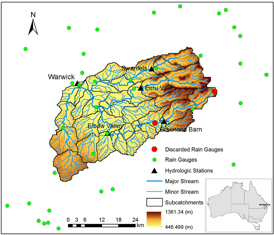
Figure 1. The study catchment and location of gauges.

Table 1 shows the data source used in this study. Five flow gauges and 35 rain gauges located within or near the catchment, with the distance to the catchment boundary ≤20 km, were used in this study. Rain gauges are relatively randomly located (one gauge per 3–4 sub-catchments). Hourly gauged rainfall data from January 4, 2007 to June 30, 2014 were obtained from the Australian Bureau of Meteorology (BoM). Daily rainfall data used as reference data in quality control were extracted from the Australian Water Availability Project (AWAP) gridded dataset. Hourly gauged discharge data were obtained from the Queensland Department of Natural Resources and Mines. The quality of the hourly rainfall archives without quality control is relatively low. The missing value percentage of the archives is about 19%. In the hydrological model, the dataset was split into three periods: the warming up period 04/01/2007–31/12/2007, the calibration period 01/01/2008–31/12/2011 and the validation period 01/01/2012–30/06/2014. There are four major floods (high flows) in the catchment during the study period, i.e., in 2008, 2011, 2013, and 2014, respectively. The splitting principle is that both calibration and validation parts content two major flood events so that the two periods can be consistent in data, and the impact of parameter changes can be avoided.

TABLE 1

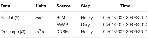
Table 1. Data source.

Methodology

Quality Control

The automated method of controlling the quality of rain gauge observations used in this study was adopted from Robertson et al. (2015). The method compares rain gauge observations with a reference rainfall data set. As discussed by Robertson et al. (2015), quality-controlled daily rainfall products, such as the AWAP gridded (5 km spatial resolution) data set, are well established for operational use in Australia. Short-term streamflow forecasting (e.g., flood forecasting), however, needs sub-daily (e.g., hourly) rainfall measurements, which are typically not well quality controlled. In this study, the AWAP daily rainfall archives were used as a reference.

The AWAP dataset was developed by the Commonwealth Scientific and Industrial Research Organization (CSIRO) and distributed by the BoM National Climate Centre (NCC), and provides interpolated datasets from 1900 till present (Jones, 2007). There are two processes in producing the AWAP dataset: the interpolation of monthly precipitation climatology with a thin plate smoothed spline, and the interpolation of daily rainfall anomalies (expressed as a percentage of the climatological rainfall with the Barnes' successive correction method (Jones and Weymouth, 1997; Mills et al., 1997; Zajaczkowski, 2009). There are no reference datasets of hourly rainfall observations. Here, the hourly gauged rainfall was firstly accumulated into daily values to be comparable with the AWAP data, and the reference daily rainfall extracted from the AWAP dataset is based on the rain gauge locations referring to the closest grid cell of AWAP.

The Pearson correlation coefficient between the daily gauged rainfall and the AWAP rainfall was used to identify gauges with poor data quality through the whole study period. Rain gauges with a correlation coefficient of <0.4 were abandoned, as suggested by Robertson et al. (2015). Incorrect time stamps can be a main reason for this problem. However, it is impossible to check and correct the time stamp (Robertson et al., 2015). Therefore, it is meaningless for the data in these rain gauges to be retained and interpolated in the next steps.

The primary target of quality control is to identify and remove spurious rain gauge observations from the entire time series that may cause poor streamflow forecasting results. Through preliminary research on the raw rainfall gauged data, anomalously large and small values were identified to have a significant impact on the hydrological modeling. Because of the large amount of data (35 observatories with more than 65,000 observations per gauge), an automatic method was used to identify the data with poor quality and implement the quality control. Specifically, through the analysis of the relationship between raw gauged rainfall (e.g., upscaled daily data) and the reference daily rainfall, the data were identified to have poor quality when the ratio of the temporal change between reference data and raw gauge data exceeded a predefined threshold (m) (Robertson et al., 2015). Those dates with poor quality data were flagged and the original hourly gauged rainfall on those dates were set to be missing. The ratio of the temporal change was calculated as

$\begin{array}{ll}s=\frac{P_{t+n}-P_{t-n}}{AWA{P}_{t+n}-AWA{P}_{t-n}},& (1)\end{array}$

where the ratio s is calculated between observed and referenced data at time t. The window used is from time t − n to t + n, with a width of 2n + 1. Based on empirical trial-and-error, the time window parameter n and the threshold m were set to be 2 (i.e., 5-day window) and 10, respectively (Robertson et al., 2015). A values of s > m indicates that the change in rain gauge observations P_t+n − P_t−n during the 5-day window were much larger than the change in the reference AWAP rainfall data AWAP_t+n − AWAP_t−n, meaning that the rainfall observation at time t + n is regarded as an anomalously large value. A value of $s<\frac{1}{m}$ indicates that the changes in the rain gauge observations were much smaller than the changes in the reference rainfall data, meaning that the rainfall observation at time t + n is regarded as an anomalously small value. The dates with anomalous daily rainfall values were flagged and the hourly gauged rainfall on those dates were removed.

The double mass curve illustrates the trends and inconsistencies of the raw and reference data, and can be used to check whether quality control has been successful (Allen et al., 1998). For each rain gauge, hourly data were summed to daily data to ensure that the time steps were consistent with the reference dataset. The AWAP rainfall data set was used as the reference to construct the double mass curve (Jones et al., 2009).

In this paper, the double mass curve was produced by plotting the cumulative sum of rainfall observations against AWAP rainfall data. The plot would be a straight diagonal line when the data are consistent. This method was used to identify inconsistencies in observation data when rain gauge observations are extremely large or small relative to AWAP data, which were reflected by vertical or horizontal segments. To construct the double-mass plots, the reference data were removed for the periods when rain gauge observations were missing (Robertson et al., 2015).

Interpolation

Many different interpolation methods can be applied to produce spatially distributed rainfall fields based on rain gauge observations. These methods can be classified into two types; deterministic methods and geostatistical methods (Ly et al., 2013). Several popular deterministic interpolation methods are used, such as IDW, nearest neighbor, and linear spline. Since most geostatistical methods are based on Kriging, the original Kriging can be used as a representative of the geostatistical interpolation. Although local terrain features may affect the performance of Kriging methods, those Kriging methods considering topography were typically applied for annual or monthly rainfall interpolation. The examination of the data used in this study indicated little correlation between the topography and the hourly rainfall records, due to large proportion of zero rainfall values. Therefore, ordinary Kriging was adopted in this study. In general, based on the weights contributed to the observed rainfall data, spatial interpolation was implemented by estimating regionalized values at the different points of a catchment, based on the weight of the regionalized observations. The general spatial interpolation function is written as

$\begin{array}{ll}P={\displaystyle \sum _{i=1}^n}{\lambda }_i\times P_i,& (2)\end{array}$

where P is the interpolated value at the centroid of a catchment, P_i is the observed rainfall data at point i, while λ_i is the weight to the observed rainfall data. In most cases, the calculation of the weights λ_i is the key problem and will be analyzed in different interpolation methods in the following sections.

Nearest Neighbor (NN)

The NN method is a simple technique where the estimated rainfall at each location P(x) can take on the observed data of the nearest gauge P(x_i). This is also called the Thiessen polygon method, which requires the construction of a Thiessen polygon network (Nalder and Wein, 1998). It is often used for thematic and dense datasets. Mediators of segments connect the surrounding gauge to other related gauges form these polygons. The surface of the polygons is used to balance the rainfall amount of the gauges at the centroids of the polygons. Therefore, once a rain gauge is inserted or removed from this network the polygon needs to be changed (Te Chow, 1964).

Inverse Distance Weighting (IDW)

The IDW method is based on the distance between the rain gauge observations and the location of the interpolated point. The weight factors are determined by the inverse of the distances. These factors are normalized so that the sum equals one. The weight factors decrease with the increase of distance, while the decrease rate become lower with the increase of distance. The power of the inverse distance function should be defined before interpolation. The lower the power, the greater the weight toward the grid point value of rainfall from remote rain gauges will be. As the power tends toward zero, this method will approximate the areal mean method (Dirks et al., 1998). As the power becomes infinitely large, the method approximates the Nearest Neighbor method (Dirks et al., 1998). In this study, the function can be expressed as

$\begin{array}{ll}\widehat{P}(x)={\displaystyle \sum _{i=0}^n}\frac{{\lambda }_i(x)}{{\sum }_{j=0}^n{\lambda }_i(x)}\times P(x_i),& (3)\end{array}$

where

$\begin{array}{ll}{\lambda }_i(x)=\frac{1}{\left|\right|x-x_i|{|}^p},& (4)\end{array}$

and x is the interpolation point; P(x_i) is the rainfall data at point x_i; the power parameter p is set to be 2 (Li and Heap, 2008).

Linear Spline (LN)

The LN interpolation method is based on a mathematical model for surface estimation that fits a linear surface (flat triangle) through the nearest three data points. It uses a “spline,” which is a piecewise linear polynomial P(x) to calculate surfaces from data points. The individual linear surfaces are connected together to form a spline surface, from which areal rainfall can be estimated (Ly et al., 2013).

Kriging

Geostatistical methods can produce smooth surfaces and evaluate their uncertainties. Kriging is a typical geostatistical method used for spatial interpolation. It is a generalized least-squares regression method, which uses observation data in a neighboring area to estimate the values at unsampled points (Hohn, 1991; Goovaerts, 1997; Deutsch and Journel, 1998). Kriging is based on statistical models involving autocorrelation, which refers to the statistical relationships between observation data (Ly et al., 2013). The value of interpolated rainfall for an unsampled location is estimated by a weighted sum of available rainfall data points, to achieve unbiased interpolation results with minimized variance.

Stationarity can be defined by constancy of the mean and the covariance between two observations. The semi-variogram, as shown in the following function, can express the “dissimilarity” of the covariance, which should be estimated and modeled before interpolation. The experimental semi-variogram can be defined as half of the squared difference between paired values to the distance that can be expressed as

$\begin{array}{ll}\gamma (h)=\frac{1}{2}\times {(Z(x+h)-Z(x))}^2.& (5)\end{array}$

With increasing h, the semivariance increases. The semivariogram can represent the change of the covariance against distance between the observation points. The raw variogram can be generated by plotting semivariances of all pairs of observations. However, the raw variogram contains noisy scatters of semivariance. The cloud of semivariance in the raw variogram can be averaged according to the gamma distribution over specified bins. It can then be converted to the experimental variogram of each bin through.

$\begin{array}{ll}\widehat{\gamma }(h)=\frac{1}{2N(h)}\times {\displaystyle \sum _{i=1}^{N(h)}}{(Z{s}_i-Z(s_i+h))}^2,& (6)\end{array}$

Statistical distribution models can be used to fit the experimental semi-variogram, while the Gaussian model is used for rainfall interpolation here such that.

$\begin{array}{ll}\gamma (h)={\sigma }^2\left(1-e^{-\frac{h^2}{L^2}}\right)=0.383\times \left(1-e^{-\frac{h^2}{900}}\right)+0.17,& (7)\end{array}$

where σ is the sill (maximum semi-variance). L is a reference distance. 7L/4 approximates to the range (correlation length), at which the semi-variance reaches the sill. For the Gaussian model, through manual curve fitting, the variance, L, and the nugget effect is estimated to be 0.383 mm², 30 km, and 0.17 mm, respectively. The coefficient in this model can be applied for the Kriging. The Kriging function can be expressed as

$\begin{array}{ll}Ẑ(x_0)-\mu ={\displaystyle \sum _{i=1}^n}{\lambda }_i\left[Z(x_i)-\mu (x_0)\right],& (8)\end{array}$

where μ(x₀) represents the sample means within the range of search window. λ_i is the kriging weight. n is the number of sampled points used to make the estimation, while μ(x₀) is the mean of samples within the study range (Li and Heap, 2008).

Hydrological Model

The hydrological model used in this study is an hourly semi-distributed hydrological model with the GR4H for runoff generation and concentration and the linear Muskingum for river routing (Li et al., 2015). The GR4H model was used in this project as it is an operational model used by BoM for their 7-day streamflow forecast service (Perrin et al., 2003; Li et al., 2014). There are two state variables, the soil water storage S (mm) and the routing water storage R (mm), and four parameters, the maximum capacity of S (x₁), the water exchange coefficient (x₂), the “reference” capacity of R (x₃), and the length parameter of the unit hydrographs (x₄). After the interception, the rainfall P (mm) contribution Pn (mm) is composed of two processes. The first process is the transformation of Pn into S, then reduced by evapotranspiration E (mm) and percolation (mm). The other process is the transformation of Pn to Ps (mm), which generates the surface runoff. Then, the surface runoff and percolation are added to form the total runoff Pr (mm). Finally, 90% of the runoff is routed by R (mm) and a unit hydrograph (UH1), while the other 10% is routed by another unit hydrograph (UH2). The ground water exchange between the modeled catchment and adjacent catchments is controlled by the function F (x₂).

Validation Methods

The method's accuracy should be investigated, which indicates how close the forecasts are to the observations (Jolliffe and Stephenson, 2012). Three statistics were used here to evaluate the accuracy of interpolation and modeling results, being Nash-Sutcliffe model efficiency coefficient (NSE) and the mean error (Bias) and the refined index of agreement (d_r) (Willmott et al., 2012; Li et al., 2015). They are described as

$\begin{array}{ll}NSE=1-\frac{{\sum }_{t=1}^T{\left(Q_m^t-Q_o^t\right)}^2}{{\sum }_{t=1}^T{\left(Q_o^t-\overline{Q_o}\right)}^2},& (9)\end{array}$

$\begin{array}{ll}Bias=\frac{1}{T}\times {\sum }_{t=1}^T\left(Q_m^t-Q_o^t\right),& (10)\end{array}$

$\begin{array}{ll}{d}_r=\{\begin{array}{c}1-\frac{{\sum }_{t=1}^T\left|Q_m^t-Q_o^t\right|}{2{\sum }_{t=1}^T\left|Q_o^t-\overline{Q_o}\right|},when{\displaystyle \sum _{t=1}^T\left|Q_m^t-Q_o^t\right|}\le 2{\displaystyle \sum _{t=1}^T\left|Q_o^t-\overline{Q_o}\right|}\\ \frac{2{\sum }_{t=1}^T\left|Q_o^t-\overline{Q_o}\right|}{{\sum }_{t=1}^T\left|Q_m^t-Q_o^t\right|}-1,when{\displaystyle \sum _{t=1}^T\left|Q_m^t-Q_o^t\right|}>2{\displaystyle \sum _{t=1}^T\left|Q_o^t-\overline{Q_o}\right|}\end{array}& (11)\end{array}$

where $Q_o^t$ (m³/s) is the observed streamflow at time t (h); $Q_m^t$ is the modeled streamflow at time t; $\overline{Q_0}$ is the temporal mean of observed streamflow and T(h) is the total validation period length.

The cross-validation method is a technique to assess the accuracy of a forecast model. In this study, the cross-validation method was used in the testing of different interpolation methods based on rainfall data, in which each gauge was interpolated using the rest of the rain gauges (Noori et al., 2014). The difference between the observed and interpolated rainfall, which indicates the accuracy, was summarized by the NSE, Bias and d_r mentioned above. The results of cross-validation methods were used to compare the accuracy of different interpolation methods.

Results

Evaluation Based on Rainfall

Quality Control

Before applying the quality control algorithm to the rain gauged observations, the correlation method was used to define gauges with poor data quality through the entire time series. The correlation results of all the rain gauges are shown in Table 2. Correlation coefficients of rain gauges 40876 (Peak) and 41537 (Killarney) observations were <0.4, and therefore these gauged observations were eliminated from the quality control and interpolation steps. Through the comparison of rainfall data with and without quality control, the relationship of correlation coefficient values and the effect of quality control can be illustrated. After applying the quality control algorithm to the rain gauged observation, all correlation coefficients increased to some extent. The average increasing of correlation is 0.0567, while at rain gauges 541061 (Cherrabah) and 541064 (Lookout), the values increase by 0.402 and 0.338, which indicates significant improvement of rainfall data. Also, the quality control impacted more significantly the rain gauges whose raw observations were of lower quality.

TABLE 2

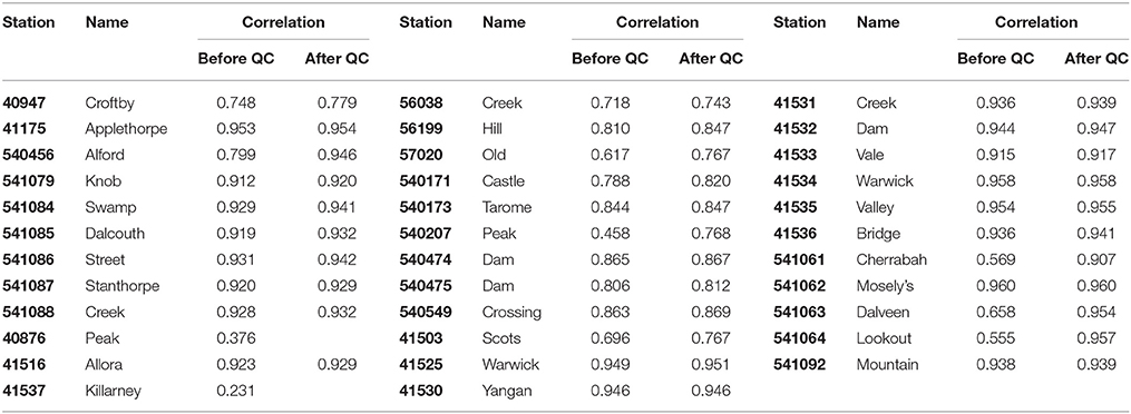
Table 2. Correlation coefficient of rain gauge observations with AWAP.

The quality control algorithm was applied to the remaining rain gauges. The impact of the quality control algorithm was found to be less significant when applied to gauges with higher correlation coefficients with the reference data. This is expected due to their consistency with the high quality AWAP data. Therefore, results are shown for gauge 540207 (Peak), where quality control was found to be important for the study period.

Figure 2 shows the double-mass plots of rain gauge 540207 against AWAP reference rainfall, i.e., cumulative gauged rainfall against cumulative AWAP rainfall. Ideally, the double mass plots should follow the 1:1 line if the gauged data have a perfect agreement with the reference. The horizontal or vertical (or near horizontal or vertical) segments reveal the gross inconsistencies. The double-mass plot of the raw rain gauge data (red line) shows that there are significant data quality issues with a long horizontal segment and some short vertical segments. The horizontal line segments indicate that during these periods, the rain gauge recorded considerably larger values than the corresponding reference data, while the vertical segments are related to occasions where the rain gauge recorded zero values which were recorded as non-zero values in the reference. The black line in Figure 2 shows the rainfall data after quality control. It is a relatively straight diagonal line without obvious horizontal or vertical segments, indicating fewer gross errors associated with quality-controlled data.

FIGURE 2

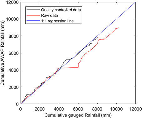
Figure 2. Double-mass plot of cumulative AWAP reference rainfall against rain gauge 540207 both before and after applying quality control.

Interpolation

The cross-validation method was used to compare the impact of the four interpolation methods directly. The NSE, Bias, and d_r calculated based on the observed and interpolated rainfall are summarized in Table 3. According to the NSE, it can be noticed that there are significant differences between the four interpolation methods, with Kriging having the largest NSE. Among all deterministic interpolation methods, IDW shows the best simulation result, whose NSE is close to the one of Kriging. Regarding the Bias, both the LN and Kriging show a better performance than the IDW and NN. According to d_r, the IDW tends to be the best with the highest d_r value. From the cross-validation point of view, both Kriging and IDW are recommended, whilst the NN gives the worst interpolation.

TABLE 3

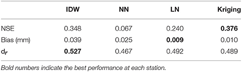
Table 3. The statistics of cross-validation for all rain gauges with different interpolation methods.

Impact on Hydrological Modeling

Tables 4, 5 show the NSE values and Bias of streamflow predictions forced by rainfall estimates obtained from the four interpolation methods and two quality control scenarios (raw/controlled).

TABLE 4

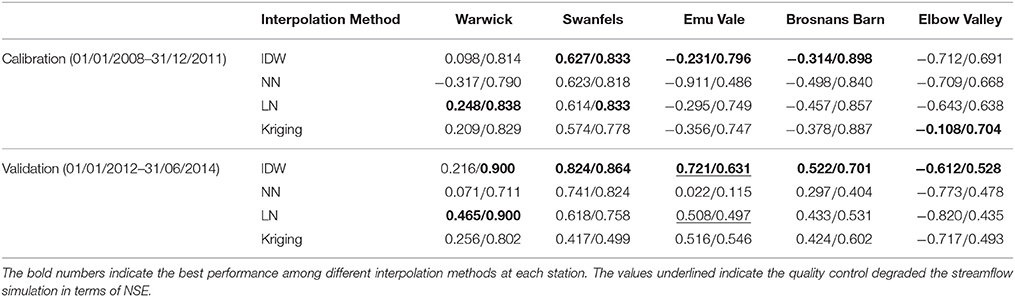
Table 4. The NSE values of streamflow predictions forced by rainfall estimates obtained from the four interpolation methods and two quality control scenarios (raw/controlled).

TABLE 5

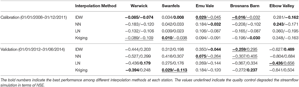
Table 5. As for Table 4 but for bias.

Impact of Quality Control

In theory, quality control of the rain gauge observations can improve the performance of the hydrological model. In this section, all four interpolation methods were used to interpolate the raw rainfall data and quality-controlled data. The raw and quality-controlled rainfall interpolations were then used to force the GR4H model for warming up (04/01/2007–31/12/2007), calibration (04/01/2008–31/12/2011) and validation (01/01/2012–30/06/2014). The NSEs shown in Table 4 indicate that in the calibration period, the model with quality-controlled rainfall data substantially outperformed the model forced by the raw rainfall data, e.g., the NSE increased from values less than zero to values close to 1. The improvements in the calibration stage are obvious in the NSE of different interpolations, which indicates an overall improvement after quality control. Especially at the Elbow Valley Station, and in the calibration stage of Brosnans Barn, all NSEs before quality control showed negative values. Improvements in the validation period are also evident, despite the fact that the NSE at Emu Vale with IDW and LN declined slightly after quality control.

Most of the absolute value of Bias shown in Table 5 decreased after quality control, indicating that simulated streamflow was generally more consistent with the real-time observations than the modeling streamflow with raw data. The improved consistency can be shown between calibration and validation periods. Consistent rainfall data play an important role in hydrological forecasting. However, in the validation stage at Emu Vale and Elbow Valley, the absolute values of Bias increased by 0.189 and 0.22 after quality control. The performance of the models calibrated using the quality-controlled rainfall data was also much more robust than the models calibrated using the raw rainfall observations, leading to improved consistency between calibration and validation results.

Figure 3 primarily compares the streamflow simulations with raw rain gauge observations and quality-controlled data at the Warwick gauge station. In Figure 3, only the effectiveness of quality control on streamflow simulation with IDW is presented. Figures 3C,D show two peak flows (wet events) in January 2011 and January 2013 in detail, respectively. For both peaks, the flow simulation with quality-controlled rainfall (blue line) matched the observation (black line) better than the simulation with raw rainfall (red line). Figures 3B,E illustrate two spurious peaks predicted by the hydrological model forced by the raw rainfall data. These significant over predictions of streamflow were eliminated by the implementation of the quality control protocol to the input rainfall. The quality control plays an important role in amendment of this phenomenon. This is consistent with the NSE and Bias results.

FIGURE 3

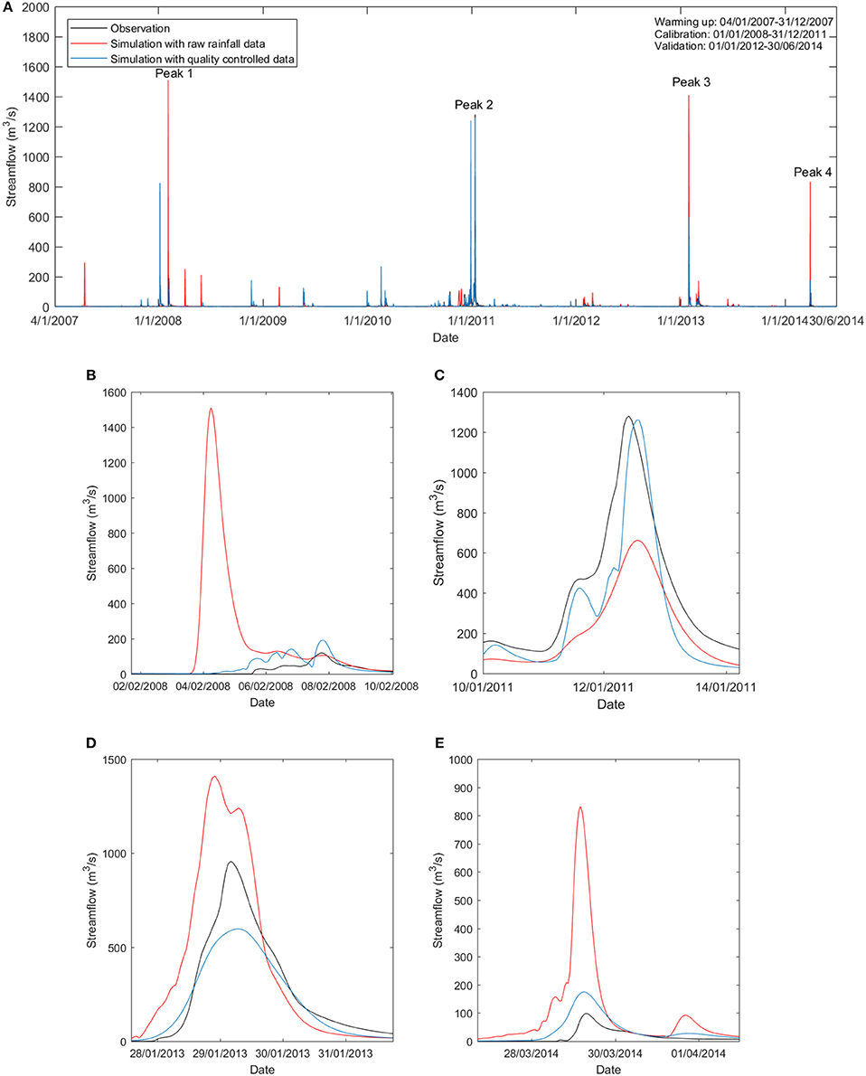
Figure 3. Streamflow of observation and simulation forced by raw and quality-controlled rainfall (IDW interpolation). (A) Streamflow during the entire timeline; (B) Streamflow peak 1 in February 2008; (C) Streamflow peak 2 in January 2011; (D) Streamflow peak 3 in January 2013; and (E) Streamflow peak 1 in March 2014.

Impact of Interpolation

According to Table 4, before quality control, IDW performed best in the calibration stage compared to other interpolation methods. However, most of the NSEs were negative, except for the Swanfels station with the NSE of 0.627. In the validation stage without quality control, IDW also showed the best results. Even at Swanfels and Emu Vale, IDW showed a NSE value which is close to one. Moreover, it can be noticed that in the calibration period after quality control, the streamflow prediction with IDW interpolated rainfall led to the highest NSE values at three gauges out of five, and in the validation period, the streamflow prediction with IDW interpolated rainfall resulted in the highest NSE value at all five gauges, indicating the IDW was the best interpolation method in this case study. According to the performance at the Emu Vale station, the Nearest Neighbor method led to the worst streamflow prediction with a NSE value in the calibration period of only 0.486, while other interpolation methods resulted in NSE values of over 0.65. In the validation stage, the NSE values for NN were the lowest at Emu Vale and Elbow Valley. Although the LN and Kriging methods showed relatively good performance during the calibration, most of NSE values during the validation were small except the one at Warwick. According to the comparison of NSE values mentioned above, the IDW interpolation method tended to be the best and most consistent interpolation method.

According to Table 5, in the calibration period before quality control, IDW showed the best result as indicated by the lowest bias at four stations out of five. In the validation stage without quality control, all interpolation methods showed similar performance at five stations. After quality control, the Bias of different interpolation methods were all negative at Warwick, Emu Vale, Brosnans Barn, and Elbow Valley. During both the calibration stage at Warwick and Emu Vale, the IDW showed the smallest absolute value of Bias, while the Nearest neighbor method had the largest Bias at most of the stations except at Emu Vale. It can be concluded that the IDW was the best interpolation method according to the Bias.

Figure 4 compares the streamflow calibration and validation results with different interpolation methods at the Warwick gauge station. Four peak flow events in February 2008, January 2011, January 2013 and March 2014 are illustrated in Figures 4B–E. These peak flow events had significant impacts on NSE. In the peak event in 2008 and 2011, all interpolation methods showed similar consistent simulation results compared with observation streamflow. However, in the event in 2013, the NN method resulted in the worst streamflow prediction. In this study, only the ordinary Kriging method was applied without consideration of local terrain features. The IDW method consistently performed well. The performance of the NN and LN methods varied from event to event. The two methods tended to be relatively accurate in the calibration events (e.g., Figures 4B,C), but failed to capture the peak flow in the validation period (e.g., Figures 4D,E).

FIGURE 4

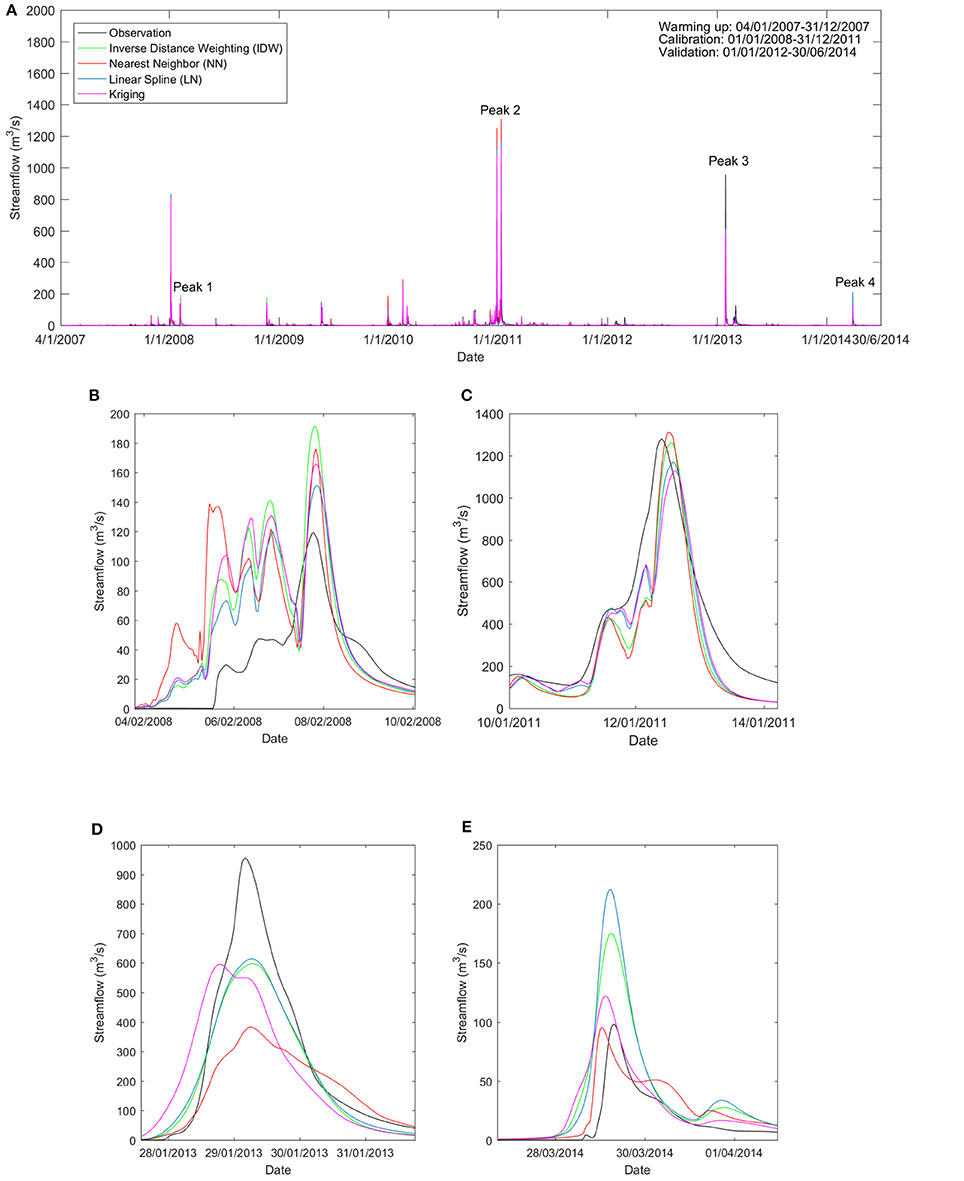
Figure 4. Streamflow of observation and simulation forced by quality-controlled rainfall with different interpolation methods. (A) Streamflow during the entire timeline; (B) Streamflow peak 1 in February 2008; (C) Streamflow peak 2 in January 2011; (D) Streamflow peak 3 in January 2013; and (E) Streamflow peak 1 in March 2014.

Discussion

In this paper, an automated quality control algorithm for hourly rainfall observations was described. Different interpolation methods were used to interpolate the rainfall observations before and after quality control. Through the assessment of the quality control method, it can be found that abnormal values significantly affect model performances, and that is consistent with some previous studies (Chaubey et al., 1999; Robertson et al., 2015). According to the cross-validation and hydrological prediction, the IDW and kriging methods resulted in the most accurate interpolated rainfall, while the NN was found to lead to the worst result. Ly et al. (2013) criticized the use of NN in mountainous regions as the orographic characteristics may have a significant impact on the rainfall distribution, which may lead to large forecasting errors (Goovaerts, 2000).

A large uncertainty in modeling results can be expected due to variations in the input rainfall (Chaubey et al., 1999). Better interpolation techniques can improve the hydrological simulations (Haberlandt and Kite, 1998). Through the NSEs analysis, it was found that if an interpolation method shows a relatively good result with raw rainfall data, it also shows a high NSE with quality-controlled data. The relative performances of all interpolation methods remained the same with raw and quality-controlled data. Although the rainfall observations before quality control were of poor quality, a relatively good interpolation method (e.g., IDW or Kriging) was not affected, due to its robustness. The less robust method (e.g., NN) was found to be affected by the quality control more significantly, with the NSE increasing from negative to positive after quality control. This was also revealed by the Bias. For instance, the quality control improved the Bias scores for NN and LN at all five gauges in the calibration period, while degraded Bias scores by quality control were found at some of the gauges for IDW and Kriging. This indicate that the NN and LN rely more on (i.e., more sensitive to) the quality control; nevertheless, the overall performances of IDW and Kriging were better than the NN and LN in terms of Bias.

It is also interesting to find that the differences between different interpolation methods using raw data were much more significant than the ones using quality-controlled data. After quality control, with the improvement of data consistency, the impact of interpolation methods tended to be lower than the interpolation results with raw observations. Considering the integrated impact of quality control and interpolation to rainfall observations, in the Elbow Valley station for example, the NSE increased significantly from negative to positive values after quality control. However, different interpolation methods show similar NSE values between −0.6 to −0.8 before quality control and 0.4 to 0.7 after quality control. It can be inferred that for the catchments with poor rainfall data achieves, the impact of quality control was more significant than the impact of interpolation methods on hydrological prediction.

Conclusions

Rainfall is the most important input for catchment hydrological modeling and has a significant impact on the accuracy of the streamflow prediction. The errors in the rainfall data applied in the calibration of hydrological models may cause poor simulations and erroneous flood forecasting results. Consequently, this paper applied an algorithm for quality control of hourly gauged rainfall data. Accordingly, the dataset with anomalously high/low or missing values was shown to be cleaned effectively, leading to an improved agreement with the reference data. Importantly, the rainfall data with quality control had a much better performance in the streamflow prediction. Four interpolation methods commonly applied to rainfall data were also reviewed and applied to the study catchments. The cross-validation, in which each gauge was interpolated using other rain gauge observations, revealed a relatively better performance for IDW and Kriging in terms of the NSE, Bias and refined index of agreements. When applied for hydrologic modeling, the IDW method gave the most accurate and robust streamflow predictions according to the NSE. The Kriging method performed second best according to streamflow predictions at the five gauges in the calibration period and four gauges during the validation period. NN produced the worst prediction at the outlet of the catchment in the validation period, indicating a low robustness. However, when evaluated in Bias, none of the interpolation methods consistently outperformed the others.

Future research is needed on the reliability of quality control methods combined with radar data. Future research may also focus on the analysis of different Kriging methods to find out whether the combination of other kriging methods and proper semi-variogram models can give better simulation results, and whether the modeling results can be improved by considering topographic features.

Author Contributions

The idea for the paper came from all authors. SL: did the quality control and interpolation, and wrote the initial draft; YL: did the hydrological modeling, and provided inputs on methodology and paper writing; VP and JW: provided inputs on methodology and result analysis, as well as comments on the paper.

Funding

This study was financially supported by the Bushfire & Natural Hazards CRC project–Improving flood forecast skill using remote sensing data. Valentijn Pauwels was funded by ARC Future Fellow grant FT130100545.

Conflict of Interest Statement

The authors declare that the research was conducted in the absence of any commercial or financial relationships that could be construed as a potential conflict of interest.

Acknowledgments

The authors acknowledge funding providers, including the Bushfire & Natural Hazards CRC and the Australian Research Council. The authors would like to acknowledge data providers, including the Australian Bureau of Meteorology for hourly gauged rainfall (extracted from BoM's internal achieve system), AWAP rainfall and PET (http://www.bom.gov.au/jsp/awap/), and the Hydrological Geospatial Fabric data (http://www.bom.gov.au/water/geofabric/), and the Queensland Department of Natural Resources and Mines for streamflow measurements (https://water-monitoring.information.qld.gov.au/). The authors also thank the editor and two reviewers for their detailed and constructive comments, which significantly improved our manuscript.

References

Allen, R. G., Pereira, L. S., Raes, D., and Smith, M. (1998). Crop Evapotranspiration-Guidelines for Computing Crop Water Requirements-FAO Irrigation and Drainage Paper 56. Rome: FAO. 300, D05109.

Australian Bureau of Meteorology (2017). Optimal Radar Coverage Areas [Online]. Available online at: http://www.bom.gov.au/australia/radar/about/radar_coverage_national.shtml (Accessed 2017).

Bell, V., and Moore, R. (2000). The sensitivity of catchment runoff models to rainfall data at different spatial scales. Hydrol. Earth Syst. Sci. Discuss. 4, 653–667. doi: 10.5194/hess-4-653-2000

CrossRef Full Text | Google Scholar

Bennett, J. C., Robertson, D. E., Ward, P. G. D., Hapuarachchi, H. A. P., and Wang, Q. J. (2016). Calibrating hourly rainfall-runoff models with daily forcings for streamflow forecasting applications in meso-scale catchments. Environ. Model. Softw. 76, 20–36. doi: 10.1016/j.envsoft.2015.11.006

CrossRef Full Text | Google Scholar

Borga, M., Degli Esposti, S., and Norbiato, D. (2006). Influence of errors in radar rainfall estimates on hydrological modeling prediction uncertainty. Water Resour. Res. 42:W08409. doi: 10.1029/2005WR004559

CrossRef Full Text | Google Scholar

Camera, C., Bruggeman, A., Hadjinicolaou, P., Pashiardis, S., and Lange, M. A. (2014). Evaluation of interpolation techniques for the creation of gridded daily precipitation (1 × 1 km2); Cyprus, 1980–2010. J. Geophys. Res. Atmos. 119, 693–712. doi: 10.1002/2013JD020611

CrossRef Full Text | Google Scholar

Chaubey, I., Haan, C. T., Grunwald, S., and Salisbury, J. M. (1999). Uncertainty in the model parameters due to spatial variability of rainfall. J. Hydrol. 220, 48–61. doi: 10.1016/S0022-1694(99)00063-3

CrossRef Full Text | Google Scholar

Chen, M., Shi, W., Xie, P., Silva, V. B. S., Kousky, V. E., Wayne Higgins, R., et al. (2008). Assessing objective techniques for gauge-based analyses of global daily precipitation. J. Geophys. Res. Atmos. 113, 1–13. doi: 10.1029/2007JD009132

CrossRef Full Text | Google Scholar

Chen, M., and Xie, P. (2008). “Quality control of daily precipitation reports at NOAA/CPC,” in 12th Conference on IOAS-AOLS (New Orleans, LA).

Google Scholar

Cheng, K. S., Lin, Y. C., and Liou, J. J. (2008). Rain gauge network evaluation and augmentation using geostatistics. Hydrol. Process. 22, 2554–2564. doi: 10.1002/hyp.6851

CrossRef Full Text | Google Scholar

Deutsch, C. V., and Journel, A. G. (1998). Geostatistical Software Library and User's Guide. New York, NY: Oxford University Press.

Google Scholar

Dirks, K., Hay, J., Stow, C., and Harris, D. (1998). High-resolution studies of rainfall on Norfolk Island: part II: interpolation of rainfall data. J. Hydrol. 208, 187–193. doi: 10.1016/S0022-1694(98)00155-3

CrossRef Full Text | Google Scholar

González-Rouco, J. F., Jiménez, J. L., Quesada, V., and Valero, F. (2001). Quality control and homogeneity of precipitation data in the southwest of Europe. J. Clim. 14, 964–978. doi: 10.1175/1520-0442(2001)014<0964:QCAHOP>2.0.CO;2

CrossRef Full Text | Google Scholar

Goovaerts, P. (1997). Geostatistics for Natural Resources Evaluation. Oxford: Oxford University Press on Demand.

Google Scholar

Goovaerts, P. (2000). Geostatistical approaches for incorporating elevation into the spatial interpolation of rainfall. J. Hydrol. 228, 113–129. doi: 10.1016/S0022-1694(00)00144-X

CrossRef Full Text | Google Scholar

Green, J., Johnson, F., Mckay, D., Podger, S., Sugiyanto, M., and Siriwardena, L. (2012). “Quality controlling daily read rainfall data for the intensity-frequency-duration (IFD) revision project,” in Hydrology and Water Resources Symposium 2012: Engineers Australia (Perth, WA), 177.

Google Scholar

Haberlandt, U., and Kite, G. (1998). Estimation of daily space–time precipitation series for macroscale hydrological modelling. Hydrol. Process. 12, 1419–1432. doi: 10.1002/(SICI)1099-1085(199807)12:9<1419::AID-HYP645>3.0.CO;2-A

CrossRef Full Text | Google Scholar

Hohn, M. E. (1991). An introduction to applied geostatistics. Comput. Geosci. 17, 471–473. doi: 10.1016/0098-3004(91)90055-I

CrossRef Full Text | Google Scholar

Jolliffe, I. T., and Stephenson, D. B. (2012). Forecast Verification: a Practitioner's Guide in Atmospheric Science. New York, NY: John Wiley & Sons.

Google Scholar

Jones, D. A. (2007). Climate Data for the Australian Water Availability Project: Final Milestone Report. Australian Bureau of Meteorology.

Google Scholar

Jones, D. A., Wang, W., and Fawcett, R. (2009). High-quality spatial climate data-sets for Australia. Aust. Meteorol. Oceanogr. J. 58, 233. doi: 10.22499/2.5804.003

CrossRef Full Text | Google Scholar

Jones, D. A., and Weymouth, G. T. (1997). An Australian Monthly Dataset, Tech Report 70. Bureau of Meteorology.

Li, J., and Heap, A. D. (2008). A Review of Spatial Interpolation Methods for Environmental Scientists. Canberra: Geoscience Australia.

Google Scholar

Li, Y., Grimaldi, S., Walker, J., and Pauwels, V. (2016). Application of remote sensing data to constrain operational rainfall-driven flood forecasting: a review. Remote Sens. 8:456. doi: 10.3390/rs8060456

CrossRef Full Text | Google Scholar

Li, Y., Ryu, D., Western, A. W., and Wang, Q. J. (2015). Assimilation of stream discharge for flood forecasting: updating a semidistributed model with an integrated data assimilation scheme. Water Resour. Res. 51, 3238–3258. doi: 10.1002/2014WR016667

CrossRef Full Text | Google Scholar

Li, Y., Ryu, D., Western, A. W., Wang, Q., Robertson, D. E., and Crow, W. T. (2014). An integrated error parameter estimation and lag-aware data assimilation scheme for real-time flood forecasting. J. Hydrol. 519, 2722–2736. doi: 10.1016/j.jhydrol.2014.08.009

CrossRef Full Text | Google Scholar

Looper, J. P., and Vieux, B. E. (2012). An assessment of distributed flash flood forecasting accuracy using radar and rain gauge input for a physics-based distributed hydrologic model. J. Hydrol. 412, 114–132. doi: 10.1016/j.jhydrol.2011.05.046

CrossRef Full Text | Google Scholar

Ly, S., Charles, C., and Degré, A. (2013). Different methods for spatial interpolation of rainfall data for operational hydrology and hydrological modeling at watershed scale. A review. Biotechnol. Agron. Soc. et Environ. 17:392.

Google Scholar

Mair, A., and Fares, A. (2011). Comparison of rainfall interpolation methods in a mountainous region of a tropical island. J. Hydrol. Engineer. 16, 371–383. doi: 10.1061/(ASCE)HE.1943-5584.0000330

CrossRef Full Text | Google Scholar

Mills, G. A., Weymouth, G. T., Lorkin, J., Manton, M., Ebert, E., Kelly, J., et al. (1997). A National Objective Daily Rainfall Analysis System, BMRC Research Report. Bureau of Meteorology.

Google Scholar

Nalder, I. A., and Wein, R. W. (1998). Spatial interpolation of climatic normals: test of a new method in the Canadian boreal forest. Agric. For. Meteorol. 92, 211–225. doi: 10.1016/S0168-1923(98)00102-6

CrossRef Full Text | Google Scholar

Noori, M. J., Hassan, H. H., and Mustafa, Y. T. (2014). Spatial estimation of rainfall distribution and its classification in Duhok governorate using GIS. J. Water Resour. Prot. 6:75. doi: 10.4236/jwarp.2014.62012

CrossRef Full Text | Google Scholar

Oudin, L., Perrin, C., Mathevet, T., Andréassian, V., and Michel, C. (2006). Impact of biased and randomly corrupted inputs on the efficiency and the parameters of watershed models. J. Hydrol. 320, 62–83. doi: 10.1016/j.jhydrol.2005.07.016

CrossRef Full Text | Google Scholar

Perrin, C., Michel, C., and Andréassian, V. (2003). Improvement of a parsimonious model for streamflow simulation. J. Hydrol. 279, 275–289. doi: 10.1016/S0022-1694(03)00225-7

CrossRef Full Text | Google Scholar

Peterson, T. C., Vose, R., Schmoyer, R., and Razuvaëv, V. (1998). Global Historical Climatology Network (GHCN) quality control of monthly temperature data. Int. J. Climatol. 18, 1169–1179. doi: 10.1002/(SICI)1097-0088(199809)18:11<1169::AID-JOC309>3.0.CO;2-U

CrossRef Full Text | Google Scholar

Štěpánek, P., Zahradníček, P., and Skalák, P. (2009). Data quality control and homogenization of air temperature and precipitation series in the area of the Czech Republic in the period 1961–2007. Adv. Sci. Res. 3, 23–26. doi: 10.5194/asr-3-23-2009

CrossRef Full Text | Google Scholar

Robertson, D. E., Bennett, J. C., and Wanga, Q. J. (2015). “A strategy for quality controlling hourly rainfall observations and its impact on hourly streamflow simulations,” in MODSIM2015, 21st International Congress on Modelling and Simulation, eds T. Weber, M. J. McPhee, and R. S. Anderssen (Gold Coast, QLD: Modelling and Simulation Society of Australia and New Zealand), 2110–2116.

Romilly, T. G., and Gebremichael, M. (2011). Evaluation of satellite rainfall estimates over Ethiopian river basins. Hydrol. Earth Syst. Sci. 15, 1505–1514. doi: 10.5194/hess-15-1505-2011

CrossRef Full Text | Google Scholar

Ruelland, D., Ardoin-Bardin, S., Billen, G., and Servat, E. (2008). Sensitivity of a lumped and semi-distributed hydrological model to several methods of rainfall interpolation on a large basin in West Africa. J. Hydrol. 361, 96–117. doi: 10.1016/j.jhydrol.2008.07.049

CrossRef Full Text | Google Scholar

Steiner, M., Smith, J. A., Burges, S. J., Alonso, C. V., and Darden, R. W. (1999). Effect of bias adjustment and rain gauge data quality control on radar rainfall estimation. Water Resour. Res. 35, 2487–2503. doi: 10.1029/1999WR900142

CrossRef Full Text | Google Scholar

Tait, A., Henderson, R., Turner, R., and Zheng, X. (2006). Thin plate smoothing spline interpolation of daily rainfall for New Zealand using a climatological rainfall surface. Int. J. Climatol. 26, 2097–2115. doi: 10.1002/joc.1350

CrossRef Full Text | Google Scholar

Te Chow, V. (1964). Handbook of Applied Hydrology: a Compendium of Water-resources Technology. New York, NY: McGraw-Hill.

Tsintikidis, D., Georgakakos, K. P., Sperfslage, J. A., Smith, D. E., and Carpenter, T. M. (2002). Precipitation uncertainty and raingauge network design within Folsom Lake watershed. J. Hydrol. Engineer. 7, 175–184. doi: 10.1061/(ASCE)1084-0699(2002)7:2(175)

CrossRef Full Text | Google Scholar

Velasco-Forero, C. A., Sempere-Torres, D., Cassiraga, E. F., and Jaime Gómez-Hernández, J. (2009). A non-parametric automatic blending methodology to estimate rainfall fields from rain gauge and radar data. Adv. Water Resour. 32, 986–1002. doi: 10.1016/j.advwatres.2008.10.004

CrossRef Full Text | Google Scholar

Vila, D. A., Goncalves, L. G. G. D., Toll, D. L., and Rozante, J. R. (2009). Statistical evaluation of combined daily gauge observations and rainfall satellite estimates over continental South America. J. Hydrometeorol. 10, 533–543. doi: 10.1175/2008JHM1048.1

CrossRef Full Text | Google Scholar

Webster, R., and Oliver, M. A. (2001). Geostatistics for Environmental Scientists (Statistics in Practice). Chichester: John Wiley & Sons.

Google Scholar

Willmott, C. J., Robeson, S. M., and Matsuura, K. (2012). A refined index of model performance. Int. J. Climatol. 32, 2088–2094. doi: 10.1002/joc.2419

CrossRef Full Text | Google Scholar

Yokoi, S., Nakayama, Y., Agata, Y., Satomura, T., Kuraji, K., and Matsumoto, J. (2012). The relationship between observation intervals and errors in radar rainfall estimation over the Indochina Peninsula. Hydrol. Process. 26, 834–842. doi: 10.1002/hyp.8297

CrossRef Full Text | Google Scholar

Zajaczkowski, J. (2009). “A comparison of the BAWAP and SILO spatially interpolated daily rainfall datasets,” in 18th World IMACS Congress and MODSIM09 International Congress on Modelling and Simulation (Cairns, QLD).

Google Scholar

Zhang, Y., Adams, T., and Bonta, J. V. (2007). Subpixel-Scale rainfall variability and the effects on Sseparation of radar and gauge rainfall errors. J. Hydrometeorol. 8, 1348–1363. doi: 10.1175/2007JHM835.1

CrossRef Full Text | Google Scholar