Cirque Glacier on South Georgia Shows Centennial Variability over the Last 7000 Years

Introduction

The accelerated melting of glaciers in the Southern Ocean (Cook et al., 2010; Scambos et al., 2014; Koppes et al., 2015) manifests rapid climate change over the last decades (Gille, 2002, 2008; Vaughan et al., 2003; Böning et al., 2008). Although anthropogenic forcing probably explains parts of this regional-scaled glacier retreat, strong regional feedback mechanisms still predominate (Thompson et al., 2011; Wang and Cai, 2013). Many of these mechanisms can be traced back to the Southern Westerly Winds, which are closely linked to the Southern Ocean's uptake of CO₂ through their effect on upwelling of carbon-rich deep water, and therefore have the potential to affect climate globally (Lenton and Matear, 2007; Le Quéré et al., 2007; Hodgson and Sime, 2010; Sigman et al., 2010). At present, the strength and position of the westerlies are rapidly shifting, but the processes behind these changes remain poorly understood, due to scarcity and of instrumental time series and paleoclimatic reconstructions (Hodgson and Sime, 2010), including glacier records which can help map out temporal and spatial changes during the Holocene.

Glaciers are established proxies of climate change (e.g., Oerlemans, 2005) and ubiquitous on Southern Ocean islands, but few reconstructions currently exists. Moreover, most work on Holocene glacier variability in the Southern Ocean is restricted to moraine chronologies (Solomina et al., 2015 and references therein). Mapping and dating of moraines provide valuable information of a glacier's extent, size, and position at points in time. However, moraine chronologies do not capture retreat phases or length of events, and cannot exclude the possibility that moraines have been erased by subsequent glacier advances of equal or larger magnitude (Balco, 2009).

The study of sediments deposited in distal glacier-fed lakes provide the opportunity to continuously reconstruct up-valley glacier variability, although not without caveats. This approach (Karlén, 1976; Bakke et al., 2010) is based on quantification of the sediment delivery by glacial erosion beneath temperate glaciers and its relationship to glacier size (Herman et al., 2015), and assumes that para- and extra-glacial material can either be ignored or identified and removed from the final glacier reconstruction, which is not always the case. Either way, larger glaciers produce more erosional products available for downstream transport by meltwater. These fine-grained glacigenic sediments settle out of suspension in downstream lakes and thus builds unremitting archives of variations in glacier size. Here we take advantage of this lake approach in an effort to produce a new and reliable glacier reconstruction from South Georgia.

The Late Pleistocene-Holocene glacier history of South Georgia has previously been reconstructed in some detail (e.g., Clapperton et al., 1989a; Gordon and Timmis, 1992; Bentley et al., 2007; Roberts et al., 2010) suggesting large Neoglacial advances. At present, only two continuous reconstructions of past glacier change exist: Rosqvist and Schuber (2003) provides a sediment record from Block lake (Husvik, Figure 1) based on gray-scale density, loss-on-ignition and grain-size spanning from 7400 to 1000 cal BP (Figure 9C), while Van Der Bilt et al. (2017) reconstruct the last 1250 years with a record from the Middle Hamberg lake (south of Grytviken, Figure 1) based on titanium counts validated against sediment density and grain size (Figure 9B). Both studies suggest centennial-scaled variability, although we do not know whether these records are representative for South Georgia. In order to enhance our understanding of Holocene glacier fluctuations on the island, we need to test if these records can be replicated.

FIGURE 1

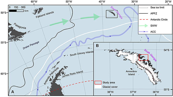
Figure 1. (A) Overview map showing South Georgia in the Southern Ocean with major circulation patterns such as the Antarctic Polar Front Zone (APFZ), the Southern Westerly Winds (SWW), and the Antarctic Circumpolar Current (ACC), as well as the Antarctic Circle and winter sea ice limit after Scar (2015) and Orsi et al. (1995). (B) Inset of South Georgia showing the current glacier extent after SGGIS (2017) and our study area.

In this study, we present a continuous reconstruction of Diamond glacier (unofficially named) on north-central South Georgia (Figure 1) covering the last 7200 years. Our glacier reconstruction is based upon measurements of physical, geochemical, and magnetic properties (cf. Bakke et al., 2010) of sediments deposited in the distal glacier-fed Diamond lake as well as the adjacent Diamond bog (both unofficially named). Mapped marginal moraines in front of Diamond glacier provide an independent framework for the past glacier fluctuations, although the timing of these moraines remains unresolved. Together, the lake-, bog- and moraine records demonstrate a consistent Holocene glacial history of Diamond glacier, which compares well with reconstructed glaciers on South Georgia and in Patagonia.

Setting

The sub-Antarctic island of South Georgia is about 170 km long and up to 40 km wide, with extensive glacier cover and an axial, alpine mountain range where mountains rise to nearly 3,000 m (Figure 1). Regional climate is influenced by the position and intensity of the westerlies, the position of the Polar Front Zone, and the Antarctic winter sea ice limit, which together mediate the temperature and moisture supply to the island (Pendlebury and Barnes-Keoghan, 2007; Figure 1). An instrumental temperature record exists for King Edward Point (KEP, c. 2 m altitude), Grytviken (Figure 2A). For the period 1905–1982, mean annual temperature was 2.0°C and mean summer (December–Feburary) temperature was 4.9°C. Mean annual precipitation was c. 1,500 mm and mean winter precipitation was 144 mm over the same time interval.

FIGURE 2

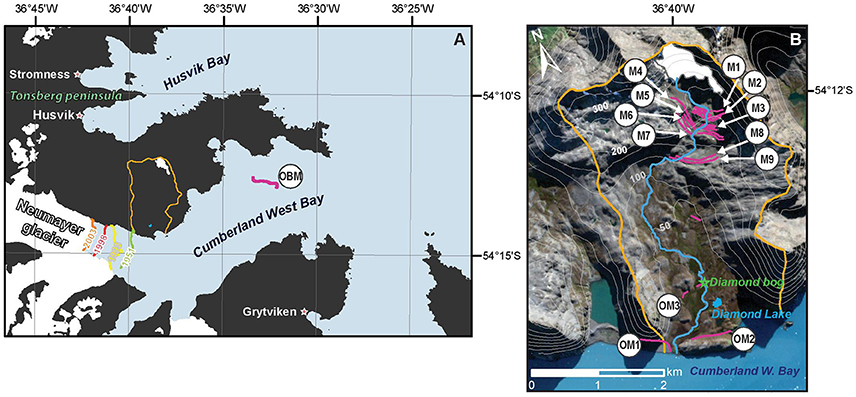
Figure 2. (A) Overview map of the Cumberland West Bay and Husvik Bay area indicating the studied catchment (orange), Diamond glacier (white), and Diamond lake (blue), as well as the Neumayer Glacier with four historical glacier front positions after SGGIS (2017), and the Antarctic Cold Reversal moraine (magenta) after Hodgson et al. (2014); Graham et al. (2017). (B) Simplified geomorphological map of Olsen Valley showing the cirque glacier (white), lake (blue), and bog (green) as well as the DB2 coring location (green star), mapped marginal moraines (pink) and the main stream (blue).

Due to a significant leeside effect on the island, glaciation on the northeast coast is restricted to small cirque and plateau glaciers, while tidewater and calving valley and outlet glaciers occupy the valleys and fjords (Figure 1; Gordon et al., 2008). According to observations, temperature is the dominant driver of glacier mass balance (Gordon and Timmis, 1992). Cirque and small valley glaciers respond most sensitively to shifts in climate, and have been receding in response to regional warming since the 1950s (Gordon and Timmis, 1992). With a delayed response, the larger valley and tidewater glaciers followed suit after the early 1970s (Gordon and Timmis, 1992), and now more than 97 % of the glaciers on South Georgia are retreating (Cook et al., 2010).

Olsen Valley in Cumberland West Bay, (Figure 2; Supplementary Figure 1) offers a favorable setting for reconstructing past cirque glacier variability using sediments deposited in distal glacier-fed Diamond lake and Diamond bog in combination with a sequence of mapped marginal moraines in front of Diamond glacier. Diamond glacier is located in a cirque southwest of the summit Diamond Peak (~510 m altitude) between c. 360 and 500 m altitude (2011) (54.20°S 36.64°W). A sequence of marginal moraines are deposited in front of the glacier, marking former glacier front positions. In the lower valley, marginal moraines mark the former glacier front positions of Neumayer tidewater glacier when it advanced into the valley from the west (cf. Bentley et al., 2007).

In the upper reaches of the valley, sediment-laden meltwater, originating from Diamond glacier, is funneled through a well-defined channel before feeding into the gently sloping valley below. The meltwater follows a course of about six kilometers down Olsen Valley before entering Cumberland West Bay (Figure 2B). The stream is intersected by an alluvial fan in the central part of the valley, containing both fresh sediments and sediments covered by vegetation, indicating deposition of glacial sediments both today and in the past. The meltwater has cut deep meanders (up to 4 m) into the bog covering the valley floor in the lower valley. Sediment sections along the river show alternating layers of peat and fine-grained sediments in the upper meter, indicating deposition of glacially derived sediments when the river floods its plains (Matthews et al., 2005).

Further downstream, the stream enters another alluvial fan separated from Diamond Lake by a marsh. The meltwater drains into the alluvial fan, which during times of moderate to high runoff has standing water. If the water level increases above c. 0.5 m, water overflows the marsh and drains into Diamond Lake. We find it likely that this occurs every year during the ablation season. The lake (54.24°S 36.65°W, 16 m altitude) covers around 10,000 m² and is ~3 m deep. Its catchment covers c.11 km², with 3% of that surface currently occupied by the Diamond glacier. Bedrock, consisting of andesitic volcaniclastic greywackes (Tanner, 1981 in Quilty, 2007), is exposed in the steeper part of the valley, which is free of vegetation, and unprotected paraglacial sediments are present in an area of c. 2 km² downstream of the glacier. The gentle slopes of the lower valley, below c. 150 m altitude, are covered by vegetation which protects the lake from mass-wasting processes. The grass Festuca contracta covers the slightly raised areas in the valley, while vegetation on the bog is dominated by the moss Tortula robusta, with grass and flowering plants present such as Acaena magellanica and Rostkovia magellanica. Following the classification of peat on South Georgia by Smith (1981), Diamond Bog is a soligenous eutrophic mire. It is developed on the floor of a broad valley and traversed by drainage channels which increases runoff and lowers the nutrient levels of the peat. At the coring site, Diamond Bog is 220 cm.

Materials and Methods

Our reconstruction of glacier fluctuations at the Diamond cirque glacier is based on a multi-proxy approach (Bakke et al., 2010), integrating geomorphological field mapping, and physical, magnetic and geochemical analyses on sediments deposited in the distal glacier-fed lake and bog.

Geomorphological Mapping

We mapped the geomorphology of the Diamond catchment (Figure 2B) based on ESA Sentinal satellite imagery (Google, n.d.)¹ combined with field surveys during January 2008 and December 2011. Our main goal was to identify marginal moraines marking former glacier coverage, and to determine past and present pathways of glacial meltwater. The topographic maps of South Georgia were, at the time of our field work, not of a resolution suitable for detailed mapping and positioning; we therefore used a hand-held GPS device (Garmin CSX60) for sites and sampling locations. The average off-set on the positions are in the order of 2–10 m.

Lake Survey and Sediment Coring

We mapped the bathymetry of Diamond lake (Figure 3) using a Garmin Fishfinder 160x echo sounder combined with a GPS and retrieved the sediment cores from the deepest and most central part of the lake (Figure 3, Table 1). For the longer piston cores (LDP1, 75 cm and LDP2, 246 cm) we used a modified piston corer able to capture up to six meters of sediments. The surface sediments at each of the two coring sites (LDS1, 34 cm and LDS2, 46 cm), we extracted using a gravity corer (Renberg and Hansson, 2008). In addition, we retrieved three sediment cores from a section of Diamond bog, upstream of the lake, by hammering PVC tubes into the bog (Figure 2B, Table 1).

FIGURE 3

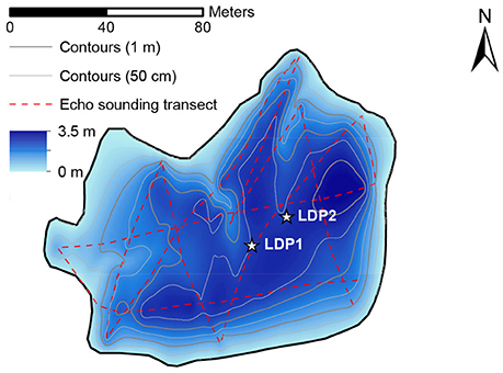
Figure 3. Bathymetry of Diamond lake indicating the echo sounding transects (red stippled lines) and coring locations for piston cores LDP1 and LDP2 in the deepest part of the lake. Gravity cores LDS1 and LDS2 were taken at the same two locations.

TABLE 1

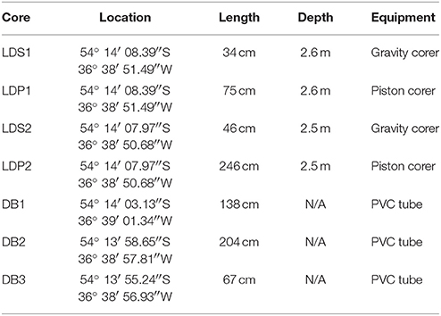
Table 1. Overview of sediment cores.

Sample Treatment and Laboratory Analyses

Prior to sub-sampling, we visually logged the lithological characteristics of the sediment cores, and used an ITRAX X-ray fluorescence (XRF) core scanner to map out the sediment geochemistry (c.f. Kylander et al., 2011). Together with the geochemical mapping at 200-μm resolution, we obtained optical and radiographic images at the same time (Figure 6). The XRF analyses were made using a molybdenum tube with power settings of 30 kV and 35 mA, employing a counting time of 10 s (N_LDP1 = 3179, N_LDP2 = 12280, N_DB1 = 6771, N_DB2 = 10201, N_DB3 = 3551).

We scanned the cores for surface Magnetic Susceptibility (MS) at 0.5 cm intervals on a Bartington MS2 point sensor (range = 0.1) (N_LDP1 = 132, N_LDP2 = 492, N_DB1 = 277, N_DB2 = 297, N_DB3 = 135). Since the gravity cores (LDS1 and LDS2) had already been sub-sampled in the field (every 0.25 cm and 0.5 cm, respectively), we measured the bulk magnetic susceptibility of these samples on a MFK1-FA (sensitivity: 2 × 10⁻⁸ SI). We use the MS data to tentatively correlate the four cores from Diamond lake (Figure 5). Being the two longest cores from, respectively, the lake and the bog, we selected core LDP2 and core DB2 for further and more detailed analyses.

We followed the protocol for Loss-On-Ignition (LOI) after Dean (1974) and dry-bulk density (DBD) after Bakke et al. (2005) of 1 cm³ dry sub-samples every 0.5 cm (N_LDP2 = 492, N_DB2 = 408). Using an MFK1-FA (sensitivity: 2 × 10⁻⁸ SI), we analyzed the mass specific magnetic susceptibility (χbulk) (Thompson and Oldfield, 1986) of discrete samples (6.8 cm³) at 1 cm intervals (n_LDP2 = ₂₃₈, n_DB2 = ₂₀₄). Prior to measurements, we freeze-dried the samples to remove the water and thereby reduce chances of post-sampling diagenesis. With the aim of distinguishing between para- and ferromagnetic sediments, we conducted the measurements at both room temperature (293 K) and 77 K (liquid nitrogen), and calculated the paramagnetic ratio (χbulk_77K/χbulk_293K) for each sample (Lanci and Lowrie, 1997).

The grain size distribution of 20 samples from LDP2 and 5 samples from DB2 were analyzed using a Mastersizer 3000 with an LV dispersion unit. All samples were pre-treated for c. 24 h with 35% hydrogen peroxide to remove the organic material (Vasskog et al., 2016) and sonicated with ultrasound for 60 s. prior to measurement. Bulk sample sizes were adjusted to have an obscuration rate of 10–20%, and measured for 10 s (blue laser) and 20 s (red laser) using refraction index of 2.5, absorption index of 0.01, and stirring rate of 2,500 rpm.

Age-depth relationships were established for the lake- and bog cores with the help of 24 individual samples of terrestrial macrofossils collected from LDP2 and DB2. Samples were submitted to Poznan Radiocarbon Laboratory for AMS radiocarbon dating (Table 2). Based on these dates, we constructed age-depth models for each core with the software package Clam 2.2 (Blaauw, 2010). We applied statistical cross-matching techniques to further constrain the age models, and to demonstrate correspondence between the three sediment cores (section Age-Depth Modeling).

TABLE 2

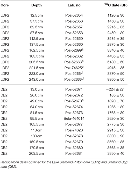
Table 2. Radiocarbon dates obtained for LDP2 and DB2.

Equilibrium Line Altitude Calculations

We constrained former glacier extents combining satellite imagery (present) with fairly intact moraines, which were mapped during the two fieldwork seasons (2008 and 2011). We used ArcMap v. 10.4 as the platform to apply the cartographic method (e.g., Ballantyne, 1989) for reconstruction of past glacier extents and surface areas. Based on this, we estimated the present and past Equilibrium Line Altitudes (ELA) of Diamond glacier (Figure 2B) using the Accumulation Area Ratio method (AAR) (Porter, 1975) with an accumulation area of 0.6 ± 0.05, which is the standard AAR value used for cirque glaciers. In addition, we used the Area x Altitude method and the Area x Altitude Balance-Ratio method (AABR) (Osmaston, 2005) with a range of balance ratios (BR) (1.5, 1.9, and 2.5) since little is known about the balance ratio in this region. The ELA reported for each moraine is the mean value of the different estimates.

Results

Moraines

We mapped nine terminal moraine ridges (M1-M9) in front of Diamond glacier (Figure 2B), which we use to reconstruct former glacier extent and calculate the corresponding ELAs (Figure 4; Supplementary Table 1). The moraines are free of vegetation, and none of them is ice-cored. We group them into four clusters described in the following.

FIGURE 4

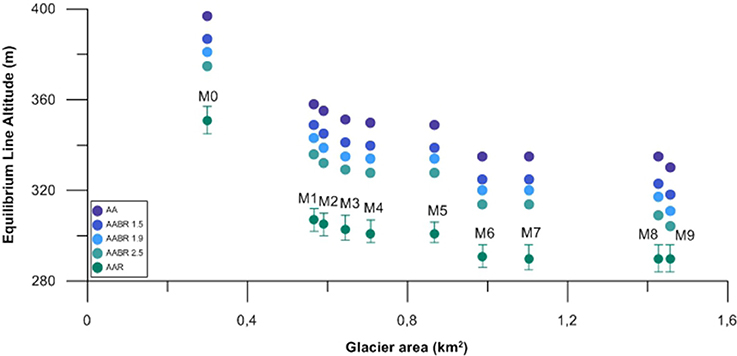
Figure 4. Reconstructed ELA for glacier stages M0 (2011) to M9 using the Accumulation Area Ratio method (AAR) (Porter, 1975), with an accumulation area of 0.6 ± 0.05, the Area x Altitude method (AA) and the Area x Altitude Balance-Ratio method (AABR) (Osmaston, 2005) with balance ratios of 1.5, 1.9, and 2.5. The ELAs are plotted against the present (2011) and reconstructed glacier areas based on glacier outlines by moraines (M1–M9).

The outermost moraine cluster (M9-M8) consists of two distinct free-standing continuous ridges (c. 2–3 m high and 300 m) located, c. 40 m apart, at a shelf (c. 170 m altitude) right before the valley drops steeply into the gently sloping lower Olsen Valley. The ridges are located at both sides of the present-day meltwater stream emerging from Diamond glacier. They consist of diamictic sediments, ranging from clay to gravel. Scattered boulders (10–30 cm in diameter) are partly embedded within or resting on the ridge surfaces. Cross sections of the moraines show an asymmetric profile with a steeper distal slope (c. 30°) and a low-angle proximal slope (c. 10°). The area distal to the ridges has exposed bedrock on both sides of the meltwater stream, which cuts through the moraines in a south westerly direction. Both ridges have undulating long profiles, which indicates partial erosion by meltwater, implying that the drainage pattern was more directly oriented toward the south when the ice front was closer to the terminal moraines. We cannot ascertain the processes of moraine formation, as no exposure in the ridge was present. At the time of moraine formation, we estimate that the ELAs were 64 ± 13 and 70 ± 12 m lower than in 2011, respectively for M8 and M9 (Figure 4; Supplementary Table 1).

The intermediate moraine cluster consists of two freestanding ridges (M7-M6), varying from 1 to 3 m in height, that continue for more than 600 m and are only cut by the river from Diamond glacier confined to a canyon (with a depth between 3 and 10 m) distal from the moraine, which funnels the meltwater toward the lower valley. Proximal to the two ridges is another partly preserved ridge (M5) that continue for approximately 550 m. Like the outermost moraines, ridges M7-M5 are composed of diamictic sediments with grain sizes ranging from clay to gravel, but with fewer boulders embedded and on the ridge surfaces. The cross profile of the ridges shows a steep distal side (c. 36°) and a more gently sloping proximal side (c. 15°). The similarities with the outermost moraine system is striking. At the time M7 and M6 were formed, ELA was 61 ± 13 m lower than in 2011, while the corresponding ELA for M5 is 47 ± 14 m (Figure 4; Supplementary Table 1).

The inner moraine cluster is located less than 50 meters proximal to ridge M5. However, the geomorphology of this moraine system is different with numerous small ridges located very close to each other. One of the ridges (M4) is freestanding and slightly higher than the others (4 m high). It can be followed over a distance of 700 m, only crosscut by the present-day meltwater stream. On the north side of M4 more than 15 small (<1 m high) saw-tooth shaped ridges can be mapped over a distance of less than 50 meters (M3). The diamicton in the moraines consists of fine sand, gravel and boulders up to 1 m in diameter. The lack of clay and fine silt indicate presence of water during deposition. Our interpretation is that the moraine cluster nested to M4, including the many smaller moraine ridges, represent an oscillatory glacier front with moraines deposited rapidly by a shrinking glacier. At the time of moraine formation, ELA was 46–47 ± 14 m lower than in 2011 (Figure 4; Supplementary Table 1).

The innermost moraine cluster consists of more than 30 individual moraine ridges deposited in a 200-meter-wide area around 320 m altitude. The two most pronounced ridges are marked M2 and M1 on the map. The ridges are between 0.5 and 1.5 meters high and are strongly asymmetrical, with a much steeper (35°) distal face and gentler (20°) proximal face. The geomorphology of the moraines is very similar to what Lukas (2012) describes as annual moraines formed when the glacier advances and acts as a bulldozer on the sediments in front. Such moraines are observed in front of several mountain glaciers on the peninsulas of north eastern South Georgia, documenting glacier retreat during the past century (Gordon et al., 2008). During the time of moraine formation, ELA was 42 ± 15 and 38 ± 15 m lower than in 2011 (Figure 4; Supplementary Table 1).

Based on GPS measurements of the glacier front during our two field campaigns, the glacier front retreated approximately 150 m between January 2008 and December 2011. This suggests that Diamond glacier follows the same pattern of rapid glacier retreat observed on South Georgia, in the sub-Antarctic, in Patagonia and indeed, globally (e.g., Cook et al., 2010; Koppes et al., 2015; Zemp et al., 2015).

In the lower valley, we mapped three moraines, covered by grasses and herbs, which outline past glacier front positions of Neumayer tidewater glacier, which advanced into the valley from the west. Parallel to Cumberland West Bay, a prominent lateral moraine (OM3), 1–4 m in height, sloping from 60 to 45 m altitude is deposited superimposed on a 100 m-high and 1 km long bedrock ridge. About 1 km further north, several cones consisting of diamict material rising above the bog likely represent remnants of a marginal moraine system (OM2). A pronounced ridge along the mountainside between Olsen Valley and the next tributary valley to the west marks a younger glacier advance (OM1). This ridge is between 2 and 6 m high and the material in the ridge is a diamicton of fine sand and boulders up to 40 cm in diameter.

Lake Sediments

Based on the correlation of the MS stratigraphy of the sediment cores from Diamond lake, (Figure 5), we argue that core LDP2 is representative for the lake. Piston core equipment sometimes fails to capture the sediment-water interface, and correlation between LDP2 and the gravity core LDS2 (taken from the same location) suggests that this is the case for LDP2. Possible overlaps between LDP2 and LDS2 were tested using a Bayesian cross matching algorithm by Werner and Tingley (2015) (Supplementary Material; Section Age-Depth Modeling), which suggests that 10 cm of the topmost sediments of LDP2 were likely lost during coring. We sub-divide LDP2 into six units (A–F) based on visual logging of the core (Figure 6A), and further divides unit F into five sub units (F1–F5) based on visual logging, grain size measurements and χbulk. Below, we give a description of each unit along with the sediment parameters LOI, DBD, χbulk, and Ti XRF count rate which we use to detect changes in the minerogenic vs. organic content in the core. The ratio of χbulk measured at 77 K and 293 K (χbulk_77K/χbulk_293K) is close to 3.8 throughout the core (Figure 6A), indicating that paramagnetic minerals dominate the samples (Lanci and Lowrie, 1997). Most values are in fact higher than 3.8, which is theoretically impossible, but can be explained. We ascribe these high values to the fact that actual temperatures of the samples when measured deviated from either 77 or 293 K, as the room might have been too cold. Samples of weak magnetic susceptibility are more prone to this error.

FIGURE 5

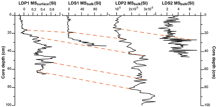
Figure 5. Intrabasin correlation based on the magnetic susceptibility (MS) stratigraphy of the piston cores (LDP1 and upper 100 cm of LDP2) and gravity cores (LDS1 and LDS2) retrieved from Diamond Lake. The stippled orange lines show the implied correlation between the cores.

FIGURE 6

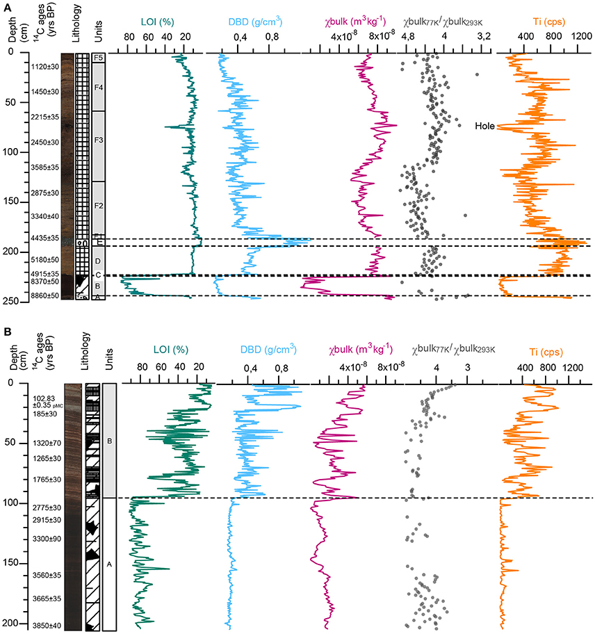
Figure 6. Selected sediment variables from (A) LDP2 (Diamond lake) and (B) DB2 (Diamond bog). Radiocarbon ages, line-scan images, sedimentary log, lithostratigraphic units, loss-on-ignition (LOI), dry bulk denisty (DBD), mass specific magnetic susceptibility (χbulk), paramagnetic ratio (χbulk_77K/χbulk_293K) and XRF titanium counts (cps).

Unit A

Unit A (243.5–246 cm) is a matrix-supported diamict, consisting of sub-angular clasts with no apparent orientation embedded in a well consolidated very dark gray matrix of clay to very fine sand (Figure 9). The clasts range in size from c. 2–20 mm and include one cobble at the bottom of the unit, measuring c. 80 mm across. The unit is characterized by high DBD, χbulk and Ti values [medians of 0.5 g/cm³, 9.0 × 10⁻⁸ m³ kg⁻¹ and 1,030 counts per second (cps)], reflecting its high minerogenic content. Based on the poor sorting and the sub-angular clasts, we interpret unit A as glacial till deposited during the last glacier retreat from the coring site.

Unit B

Unit A grades into unit B (223–243.5 cm), a dense, structureless and highly decomposed very dark brown peat with one laminae of sandy silt at 230 cm. The high organic content of the unit is reflected by high LOI values (median of 80 %) corresponding with low values of DBD, χbulk, and Ti (medians of 0.1 g/cm³, 2.8 × 10⁻⁸ m³ kg⁻¹ and 80 cps). We interpret unit A to represent a peat bog environment with little (glacio-) fluvial influence.

Unit C

A sharp erosive bedding plane separates unit B from unit C (221.5–223 cm), a very thin bed of dark gray moderately sorted sand, with sub-rounded grains ranging from c. 1–5 mm, and containing one wood fragment (10 mm long, 5 mm in diameter). The unit is best resolved in the high-resolution XRF counts, with high Ti counts around 1,000 cps, reflecting the minerogenic nature of the sediments. Based on the sediment texture and wood fragment, we interpret the unit to represent a flooding event, causing erosion into unit B. According to our age-depth model (Figure 7), the resulting unconformity represents a hiatus of ~2000 years.

FIGURE 7

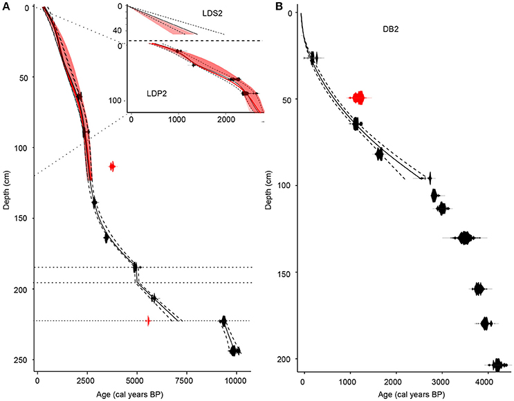
Figure 7. Age-depth models for (A) LDP2 and LDS2 (lake), and (B) DB2 (bog). Each calibrated ¹⁴C age range is shown in black. Outliers are displayed in red. The Clam models are represented by solid black lines, with broken black lines marking the 95% confidence bands. Horizontal stippled black lines mark the slump between 185 and 195 cm, as well as the hiatus at 223 cm in LDP2. The dark red lines mark the best fitting age models for LDS2 and the upper 95 cm of LDP2, which were constrained using Bayesian statistics. Bands in a lighter red and pink shade marks the 50 and 95% confidence intervals, respectively.

Unit D

Unit C has a sharp bedding contact with Unit D (194–221.5 cm), which consists of a dark grayish brown organic-rich silt with grain sizes ranging from clay to medium sand (Figure 9). The sediments are well consolidated (median DBD of 0.6 g/cm³), and small plant fragments are dispersed throughout the unit (median LOI of 11 %). The high minerogenic content is reflected by high median values of DBD, χbulk (7.9 × 10⁻⁸ m³ kg⁻¹) and Ti (930 cps) (Figure 5). We interpret unit C to represent glacial flour (clay and silt) and reworked sediments (sand) deposited in a lake.

Unit E

A sharp undulating non-erosive bedding contact separates unit D from unit E (185.5–194 cm), which is composed of a poorly sorted very coarse dark gray loosely consolidated sand containing sub-angular pebbles up to 30 mm across and no silt or clay particles. The high minerogenic content is reflected by low LOI values (median of 2%) and high values of DBD (median of 1.1 g/cm³), Ti (median of 960 cps) and χbulk (one bulk measurement of 4.0 × 10⁻⁷ m³ kg⁻¹) (Figure 5). We interpret unit E as a slump, formed by mass wasting of sediments from a moraine.

Unit F

Unit F (0–185.5 cm) consists of dark brown to dark grayish brown organic-rich sediments with dominant grain sizes ranging from clay to fine sand. We interpret unit F to represent a lake similar as today, into which the meltwater stream carried glacially eroded silt and clay directly from the glacier, but also remobilized coarser grain fractions as well as terrestrial plants in the catchment during times of high runoff. We argue that the input of minerogenic sediments to the lake is positively correlated with glacier size (Section Reconstructing the Glacier). Based on variations in color, minerogenic content, χbulk, grain size distribution, and organic content, we divide unit F into five sub units (F1–F5).

Unit F1 (185.5–182 cm) is a dark grayish brown organic-rich silty sand displaying similar characteristics as unit D, but is dominated by sand, rather than silt. It was likely deposited under similar environmental conditions as unit D, but also affected by the preceding mass wasting event (Unit E). One grain size measurement at 182 cm shows that very fine sand dominates, and median χbulk is 8.1 × 10⁻⁸ m³ kg⁻¹.

Unit F2 (182–128 cm) consists of consolidated organic-rich sandy silt with a dark grayish brown color, interspersed by lamination of well sorted very fine sand at 181, 153, 148, 146, 137, and 134 cm. Grain size measurements reveal a bimodal distribution with peaks around very fine sand and medium silt (Figure 9). The finer fractions indicate input of glacial sediments while the sand is likely remobilized paraglacial sediments from the fan next to the lake. Throughout the unit, χbulk generally decreases. Values are low (median of 6.4 × 10⁻⁸ m³ kg⁻¹), but increases over the sand layers (Figure 6A).

Unit F3 (128–58 cm) is a dark brown organic-rich silty sand with high content of moderately decomposed plant fragments. The grain size distribution of four samples (118, 88, 70, and 65 cm) peaks around very fine sand, but silt is also present. χbulk generally increases through the unit (median of 8.0 x 10⁻⁸ m³ kg⁻¹). Between 71 and 75 cm, large terrestrial plant fragments (likely the herb Aceana magellanica/tenera) are found at the center of the core, probably representing a flooding event, with the high organic content of the layer reflected in a drop in the DBD and χbulk values (Figure 6A). Part of this organic material fell out when splitting the core into two half tubes. The resulting hole caused very low XRF counts (190 cps) as the detector was not close enough to the sediment surface (Figure 6A). Terrestrial plant fragments are found at several depths in the unit (e.g., 86, 97, 110, and 120 cm). The terrestrial plant remains and coarse grain sizes indicate a high energy system causing remobilization of sediments and terrestrial organic material in the catchment, and subsequent deposition into the lake. While sand settles in the lake, the finer fractions are transported all the way into Cumberland West Bay.

Unit F4 (58–10 cm) is dark grayish brown organic-rich silt. Grain size measurements at 55, 33, 24 and 14 cm show dominating clay and silt fractions. At 44 and 48 cm, fine sand dominates but the finer fractions are also present. In the lower 24 cm χbulk values are comparable to unit D and F1, but starts to decrease from 5.6 × 10⁻⁸40 cm, reaching around 13 cm with χbulk (5.6 × 10⁻⁸ m³ kg⁻¹). We interpret this unit to represent lower energy conditions than in unit F3. The presence of clay and silt indicate input of glacial sediments. According to χbulk glacial input is high, comparable to that of unit D, between c. 58 and 38 cm, but decreases through the rest of the unit. Deposition of remobilized sand occurs at some intervals, indicating events or short periods of higher run-off.

Unit F5 (10–0 cm), consists of dark brown organic-rich silty sand (Figure 10) with a high content of woody plant fragments, increasing toward the top. The grain size distribution of one sample at 3 cm peaks around very fine sand, similar to unit F3, but the silt (and clay) content is a little higher. χbulk increases through the unit from 5.6 × 10⁻⁸ to 7.3 × 10⁻⁸ m³ kg⁻¹. We interpret unit F5 to represent a system of increasingly high run-off, where both clay and silt from the glacier as well as remobilized sediments and terrestrial organic material from the catchment are deposited in the lake.

Bog Sediments

During the coring of the DB2, we measured compaction due to the friction in the corer to be ~16 cm, but since we know little about how the compaction was distributed through the core, we do not attempt to correct for it. We sub-divide DB2 into two units (A and B) based on visual inspection of the core (Figure 6B).

Unit A

Unit A (95–204 cm) is composed of dense, highly decomposed black peat with laminations of clayey silt at 100 and 155 cm. The high organic content is reflected in the high median value of LOI (87 %) and low median values of DBD, χbulk and Ti (0.2 g/cm³, 1.0 × 10⁻⁸ m³ kg⁻¹ and 90 cps) (Figure 6B). We interpret unit A to represent a peat bog environment with little influence of glacial meltwater.

Unit B

Unit A grades into unit B (0–95 cm), which consists of very dark brown clayey peat interbedded with gray to grayish brown layers of fine minerogenic material and fragments of moss and rootlets. Bedding planes are indistinct, and bed thicknesses vary from <1 mm to 5 cm, with three 3–5 cm thick layers in the upper 25 cm of the unit. Using the XRF count ratio Fe/Ti, we identified 33 minerogenic layers in unit B, which we confirmed by inspection of the sediments. The grain size distribution of four minerogenic layers at 3–5, 6.5–10, 18.5–23, and 73–74 cm, reveal a domination by silt and clay. At the bottom of the unit (94 cm) grain sizes are dominated by very fine to fine sand in addition to a high content of silt and clay. The organic content of the unit is moderately to poorly decomposed, with the degree of decomposition decreasing toward the top of the core which preserves the topsoil. Compared to unit A, the measured sediment parameters show higher variability in Unit B, reflecting the variable content of minerogenic vs. organic material. LOI varies between 4 and 88%, DBD varies between 0.2 g/cm³ and 1.1 g/cm³, χbulk varies between 3.0 × 10⁻⁹ m³ kg⁻¹ and 5.8 × 10⁻⁸ m³ kg⁻¹, and Ti varies between 210 cps and 1460 cps. The paramagnetic ratio is close to 3.8 throughout the unit (Figures 6B, 10), indicating one main sediment source (Section Lake Sediments). This, together with the grain size distribution of the minerogenic layers and the transport of glacial meltwater through the bog in a deep channel, suggests that the minerogenic layers in the bog are composed of glacial sediments. We interpret unit B as a peat bog environment such as today, where glacially eroded sediments are deposited onto the bog when the river overflows its banks. The high content of sand in the bottom of the unit concurs in time with the increased sand input to the lake (Section Reconstructing the Glacier) and infers higher energy in the system.

Age-Depth Modeling

We established age-depth relationships for LDP2, LDS2, and DB2 (Figure 7) in the following steps (for more details on the approach see Supplementary Material):

1) Based on the 24 radiocarbon ages (Table 2; Figure 6) we constructed independent age-depth models for LDP2 and DB2 using the software Clam 2.2 (Blaauw, 2010), with the SHCal13 calibration curve (Hogg et al., 2013) and post-bomb curve 4 for zones 1–2 (Hua et al., 2013), generating 2000 iterations for each core. Owing to stratigraphically inverted ages, we excluded radiocarbon samples Poz-52659 (LDP2), Poz-74625 (LDP2), and Poz-52673 (DB2) from the age models (Table 2). Poz-52659 and Poz-52673 were excluded based on their improbable old ages and the small sample size of Poz-52673. We chose to exclude Poz-74625 rather than Poz-52664 because we deem the resulting sedimentation rate to be more likely as visual inspection of the sediments reveal no major changes in this interval. We interpret and treat unit E (185.5–194 cm) in LDP2 as a slump (section Lake Sediments) because of its gravel content and erosional contact with unit D. Based on the sudden jump in age, we infer an unconformity between unit B and C. We therefore made one set of age models for units D-F (upper 221 cm), and one for unit B. To obtain the best goodness-of-fit, we applied a smooth spline interpolation for the upper 221 cm (Figure 7A). With only two ages in unit B, we were left with the option of linear interpolation between them. We constrained the DB2 age model by an assumed surface age of −61 year. BP (2011 AD), the year of coring. Owing to the low concentration of minerogenic sediments in unit A, we only use unit B in step 2 and 3 below. We therefore applied a smooth spline interpolation between the ages for unit B only (Figure 7B).

2) Assuming that both cores are now on correct age scales, they likely record the same minerogenic events. We used the ratio of Fe/Ti to identify 33 minerogenic layers in the upper 95 cm of DB2 (Supplementary Figure 2), and compared them to sediments in LDP2 representing the same age intervals. In Figure 8, we show the Fe/Ti ratios of the minerogenic layers in DB2 vs. the Fe/Ti ratios for the corresponding layers in LDP2. Based on the good correspondence between the two records, we argue that we can use the age model of DB2 to further constrain the last 2700 years of the age model of LDP2.

3) We used a modified version of the algorithm by Werner and Tingley (2015), to statistically cross-match LDP2 and DB2, and further constrain the uncertainties of the LDP2 age model. The motivation behind the algorithm is that the variables of the records should respond to the same environmental driver—in this case glacier fluctuations—and that thus the common variability expressed in the used variable can be used to cross-match the cores within the allowed uncertainties of the age-depth models. The result of the cross-matching is shown in Supplementary Figure 3.

4) From cross-matching LDP2 and LDS2 by eye (Figure 5), we argue that the top sediments of LDP2 are missing. In order to extend LDP2 to the present, we constructed an age model for the undated core LDS2 based solely on the sedimentation rates inferred for LDP2. Using the aforementioned algorithm, we tried to reconcile the possible age models for LDP2/LDS2 (Supplementary Figures 5, 6).

FIGURE 8

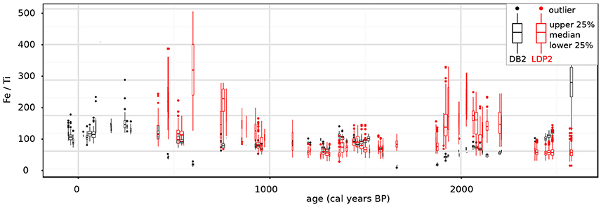
Figure 8. Comparison of layers with high minerogenic content in DB2 (black) with sediments corresponding to the same time intervals in LDP2 (red), covering the past 2700 years. We used high-resolution XRF counts (0.02 cm) to be able to resolve the layers, which are here represented by Fe/Ti. The box plots indicate the range of Fe/Ti values within each layer. The width of the box plots indicate the thickness of each layer. DB2 extends beyond LDP2 due to the missing topmost sediments of LDP2.

Discussion

Reconstructing the Glacier

There is a long tradition for utilizing downstream basins as sedimentary archives for reconstructing glaciers dating back to pioneering work by Karlén (1981). Since these early studies, progress have been made regarding the methodological tool-kit invoked in order to track past glacier activity (e.g., Bakke et al., 2010) as well as tools for precise modeling of the age-depth relationship based on ¹⁴C dates, ²¹⁰Pb dates and tephra (Blaauw, 2010) ensuring robust chronologies. One of the challenges with lake-based glacier reconstructions is the necessity of recognizing various catchment processes that potentially can impact downstream sedimentary records (Rubensdotter and Rosqvist, 2005; Bakke and Paasche, 2011). To disentangle the different processes acting on the archives, it is increasingly common to employ multiple proxies (e.g., Bakke et al., 2010; Vasskog et al., 2012). Sediment variables, commonly reflecting the glacial signal include elements such as Si, K, Ca, Ti, Fe, Rb, and Zr (Davies et al., 2015), variations in bulk organic matter as given by loss-on-ignition (e.g., Karlén, 1976), DBD (e.g., Bakke et al., 2005) and grain size (e.g., Matthews and Karlén, 1992), as well as a range of magnetic properties (e.g., Paasche et al., 2007). In this study, we use mass specific magnetic susceptibility (χbulk) as an indicator of change in the suspended glacigenic input to the bog and lake. Magnetic susceptibility is a measure of the magnetic minerals in a sample which is closely related to the concentration of minerogenic material (Thompson et al., 1975; Thompson and Oldfield, 1986). The approach of using χbulk as a proxy for glacier variations is validated by the positive correlation of χbulk with DBD, surface magnetic susceptibility and common detrital elements such as K, Ca, Ti, V, Mn, Fe, and Sr (Supplementary Table 2).

Olsen Valley represents a relative simple system where a single river drains a small upstream cirque glacier, feeding meltwater through the lower valley from a point source. Given the high ablation season temperatures (mean T_Oct−Apr = 3.6°C) we assume that the glacier is temperate and also remained temperate during the period covered by our sediment record (last 7200 years). We neither find geomorphological evidence, such as ice-cored moraines, that the glacier was cold based or polythermal during this period, nor are such previously reported from the island. For the sake of comparison, polytemperate glaciers in Scandinavia and Greenland typically have mean ablation temperatures around 1°C or colder (Østrem et al., 1988; Weidick, 1992). Such a decrease in temperature is highly unlikely for the Holocene on South Georgia, as indicated by the GDGT temperature record by Foster et al. (2016) and the δD temperature record from the Antarctic Peninsula by Mulvaney et al. (2012). The size variations of temperate glaciers are typically positively correlated to the production and evacuation of glacial sediments (Herman et al., 2015).

We regard the minor minerogenic content in the bog during the late Holocene climate optimum (4800 ± 200 to 2700 ± 150 cal BP, section Glacier retreat: 4800 ± 200 to 2700 ± 150 cal BP), when the glacier is inferred to be very small, as evidence that the glacier is the main driver of the sediment variability in the bog (Matthews et al., 2005). The sediment influx to the bog and lake is predominantly associated with the ablation season (summer) when increased runoff causes the river to transport and subsequently deposit glacial flour in the bog and lake. Based on the low mean summer precipitation (mean P_JJA = 105 mm), we argue that the additional extra-glacial sedimentary delivery from the other parts of the catchment is small compared to that which stems from glacial meltwater. There exsists no record of extreme precipitaiton events from South Georgia, however such events can cause inwash of inorganic sedimentation to our sites and is a possible error source for our interpretations. Sitting in a gently sloping valley covered by vegetation, we consider mass wasting processes not likely to affect the bog and lake.

While the gently sloping part of the valley is covered by peatland, thereby limiting the possibility of reworking of older sediments (paraglacial activity), glacigenic deposits closer to the glacier, as well as in three fans deposited in the lower valley, are potentially available for erosion and thus re-mobilization (Ballantyne, 2002). This could potentially be a source of error when using the sediments to reconstruct the up-valley glacier. Still, since sedimentation into the bog and lake happens mainly during the ablation season, we argue that re-deposition of paraglacial sediments would only reinforce the glacier signal rather than distort it. The presence of fine sand in the lake (Figure 9) indicates that there is indeed a paraglacial component present. These sediments are likely remobilized from the alluvial fan to the west of the lake during periods of high runoff. This is supported by the domination of clay and silt in the bog, which is located up valley from the fan, suggesting low paraglacial input. Sand in the bog is limited to an interval between 93 and 95 cm (c. 2700–2400 cal BP). This interval concurs in time with increased sand input to unit F3 (2700 ± 150–2000 ± 200), suggesting that both lake and bog received paraglacial sediments from up valley sources (likely the alluvial fans) between 2700 ± 150 and 2000 ± 200 cal BP when runoff was at its highest in the last 7200 years.

FIGURE 9

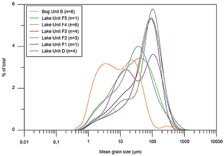
Figure 9. Distribution of mean grain-size values of the analyzed samples (n) in unit D and F1–F5 of Diamond lake as well as Unit B of Diamond bog.

Seeing as both the bog and lake receive input of glacigenic material during periods of high river discharge, we claim that the two records should co-vary in phase over time. This assumption is confirmed in Figure 8, which shows increased χbulk in LDP2 corresponding in time with the 33 silt layers identified in DB2. This relationship serves to validate the lake record and demonstrates the potential in using distal-glacier fed bogs as archives of glacier variability. Other lines of evidence also suggest that the lake and bog capture the same glacial history. The paramagnetic ratios (χbulk_77K/χbulk_293K) of LDP2 and DB2 indicate that both records are dominated by paramagnetic minerals (Lanci and Lowrie, 1997) (Figure 11; section Lake Sediments) and that this doesn't change during the period in question. This shows that the minerogenic material deposited in the lake and bog derives predominantly from one source only, unless one assumes that the signal is the same for the entire catchment, which is unlikely considering the geological processes involved. Further supporting evidence is the overlapping grain size distributions of the bog and lake. Characteristic of glacial flour, we argue that the source of the minerogenic and fine-grained sediments is erosion by the Diamond glacier, which, drawing from moraine evidence, was present in the catchment during the Holocene.

The mapped moraines in front of Diamond glacier provide spatial constraints for the glacier fluctuations reconstructed from the sediments, as we arguably detect the documented glacier advances of the LIA and in the 1930s both in the sediment records and in the moraine sequence. Based on previous studies from South Georgia, we argue that M1 was deposited during the 1930s while M2 was deposited during the Little Ice Age (LIA). An extensive glacier advance during the LIA (seventeenth to ninetieth centuries) is well-documented on the peninsulas of northeastern South Georgia (Gordon and Timmis, 1992). Clapperton et al. (1989b) estimate an average ELA depression of c. 50 m during this period, corresponding with a cooling of 0.5°C. Within the uncertainty range, this is comparable to the ELA of M2. Proximal to the LIA moraine it is common to find a moraine deposited during the twentieth century (Gordon and Timmis, 1992). This advance was documented by historical evidence (Hayward, 1983), showing that many glaciers advanced in the twentieth century. Cirque and valley glaciers were at its most advanced position in the 1930s, while larger valley and tidewater glaciers reached their maximum glacier extent in the 1970s. Such a glacier advance is also documented for the Hamberg glacier by Van Der Bilt et al. (2017). Furthermore, during the recession phase after the twentieth century advance, many cirque glaciers deposited annual moraines (Gordon and Timmis, 1992), such as the ones observed in the innermost moraine cluster. Thus, Diamond glacier followed a similar pattern to that observed for small glaciers (0.1–4.0 km²) on South Georgia during the late Holocene, with a Little Ice Age advance, a period of recession, a twentieth century advance and a recent recession (Gordon and Timmis, 1992). Based on the lake sediments, we argue that M8 and M9 were deposited prior to lake formation 7200 ± 400 years ago. We assume that the glacier would produce a distinctly higher χbulk in the lake at this time (being 30% larger than the glacier which deposited M7). The lake record, however, indicates that the glacier repeatedly reached close to its maximum Holocene position (Figure 11).

Holocene Glacier Variability in Olsen Valley

In the following we present the reconstructed Holocene glacier variability in Olsen Valley as interpreted from the lake and bog sediment records and linked to the moraine sequence based on previous studies of glacier front positions on South Georgia (section Reconstructing the Glacier). We use χbulk as a proxy for glacier size, except in the topmost part of the lake record where we use κbulk (see section Sample Treatment and Laboratory Analyses). Since we combine two different measures of magnetic susceptibility in the lake, we standardize the χbulk and κbulk results (Figure 11A). To account for glacier response time, we apply 30-year bins in the presentation of the glacier reconstruction following Van Der Bilt et al. (2017).

Deglaciation of Lower Olsen Valley: < 9900 ± 250 cal BP

Based on the onset of peat accumulation in Diamond lake, lower Olsen valley was ice free prior to 9900 ± 250 cal BP. We argue that the diamicton found in Unit A (LDP2) was deposited by the Neumayer Glacier, as moraines OM2 and OM3 outline a glacier advance from the west (Figure 2B) (Bentley et al., 2007). This is supported by the slightly lower values of χbulk_77K/χbulk_293K in Unit A compared to the rest of the record (Figure 6A), indicating a different sediment source. A retreat of Neumayer Glacier from Olsen Valley before 9900 ± 250 cal BP agrees with radiocarbon dates of peat and lake bases in the Cumberland Bay and Stromness Bay area (cf. Van Der Putten and Verbruggen, 2005) suggesting that the lower zone (<50 m a.s.l.) was deglaciated in in the first centuries of the Holocene.

Marine evidence connects OM1 and OM2 to the glacier retreat following the Antarctic Cold Reversal on South Georgia (15 170–13 340 cal BP). Hodgson et al. (2014) document a partially preserved moraine in the outer basin of Cumberland West Bay (Figure 2A). This moraine is associated to the Antarctic Cold Reversal advance on South Georgia by Graham et al. (2017) who dated the transition from subglacial to ice-proximal sediments in a core taken through the equivalent moraine in Cumberland East Bay to 13,340 cal BP. Another date from the same sediment core suggests nearby glacier sources at the outer basin moraine until c. 10,600 cal BP (Graham et al., 2017). Based on the above dates, we suggest that OM2 and OM3 were deposited between c. 10,600 and 9900 ± 250 cal BP.

Glacier Advance: 7200 ± 400 to 4800 ± 200 cal BP

We have evidence of continuous peat formation and dry land conditions until 9350 cal BP, but the unconformity between unit C and D makes it difficult to establish when the lake formed, as we have no account of what happened between 9350 and 7200 ± 400 cal BP. The period between 7200 ± 400 and 4800 ± 200 cal BP (unit D) is characterized by high input of clay and silt (Figure 9). Characteristic of glacial flour, these fine-grained sediments were transported in suspension by glacial meltwater directly from the glacier. We interpret the high χbulk values to represent a glacier close to its maximum Holocene position (Figure 11A). In line with our findings, evidence from bryophytes and seeds on nearby Tønsberg Peninsula (Figure 2A; Van Der Putten et al., 2004) suggests cold and wet conditions between 7000 and 4000 years BP, which would favor glacier a during this period.

Glacier Retreat: 4800 ± 200 to 2700 ± 150 cal BP

From 4800 ± 200 cal BP χbulk decreases and remains low until 2700 ± 150 cal BP (Unit F2, Figure 6A, Figure 11A). In Diamond Bog median LOI is close to 90% (Figure 6B), suggesting that the bog was isolated from meltwater input (Figure 10). However, the presence of clay and silt in Diamond Lake (Figure 9) suggests that the glacier was present in the catchment, and had not completely melted away. Evidence for a contemporaneous Late Holocene climate optimum on South Georgia has been found in several studies, reporting reduced glacier activity (Rosqvist and Schuber, 2003) higher temperatures (Clapperton et al., 1989a; Strother et al., 2015; Foster et al., 2016) and a drier climate (Van Der Putten et al., 2004, 2009). Paleoclimatic records from other sub-Antarctic locations such as the Antarctic Peninsula (Sterken et al., 2012), Livingstone Island (Björck et al., 1991), South Shetland Islands (Björck et al., 1993), and James Ross Island (Mulvaney et al., 2012) demonstrate consistent climate change over a wide region.

FIGURE 10

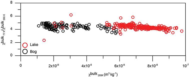
Figure 10. The mass specific magnetic susceptibility (χbulk_293K) plotted against the paramagnetic ratio (χbulk_77K/χbulk_293K) for the lake (red) and bog (black) sediments show that both records are dominated by paramagnetic minerals, indicating one main sediment source.

Glacier Advance: 2700 ± 150 to 2000 ± 200 cal BP

From 2700 ± 150 cal BP we see a sudden shift in the sedimentary regime of both the bog and the lake. Large amounts of sand and silt suddenly starts to wash into the bog (Figure 6B). Sand, silt and terrestrial plants are deposited in the lake (Unit F3, Figure 6A), and modeled sedimentation rates increase in both records (Figure 7). We interpret this shift to mark a sudden transition from warm and dry climate conditions with restricted glaciation to a wetter and colder period favoring glacier advance. The energy in the hydrological system of the valley is high, as indicated by the coarser grain fractions and the input of terrestrial organic material, and the contribution of precipitation vs. glacier advance to the increased χbulk values are difficult to disentangle. However, based on the sensitive response of present cirque glaciers on South Georgia (Van Der Bilt et al., 2017), we find it likely that Diamond glacier advanced within short time after 2700 ± 150 cal BP. The change in the sediment records coincides with a shift in climatic conditions, which is recorded in various proxy records from South Georgia. Clapperton et al. (1989a) dated moraines on north-central South Georgia to around 2000 cal BP. Rosqvist and Schuber (2003) document cirque glacier advance at the same time in Husvik (Figure 2A), while evidence from changes in pollen and macrofossils from Tønsberg Peninsula (Figure 2A; Van Der Putten et al., 2004, 2009) and Annenkov Island (Figure 1; Strother et al., 2015) mark a sudden change in vegetation in response to cooler and wetter conditions from around 2700 cal BP, and Foster et al. (2016) infer cooling on Annenkov Island based on glycerol dialkyl glycerol tetraethers (GDGTs) (Figure 11E). The shift to a cool and wet climate around 2700 cal BP also falls in line with evidence of a major glacier advance prior to 2600 cal BP in the south-central Andes (Grosjean et al., 1998). On James Ross Island, temperatures starts to decrease after 3000 cal BP (Mulvaney et al., 2012; Figure 11F), while evidence of peat growth initiation since 2800 cal BP suggests warmer summers in the western Antarctic Peninsula (Yu et al., 2016), demonstrating the Antarctic dipole (Yuan, 2004).

FIGURE 11

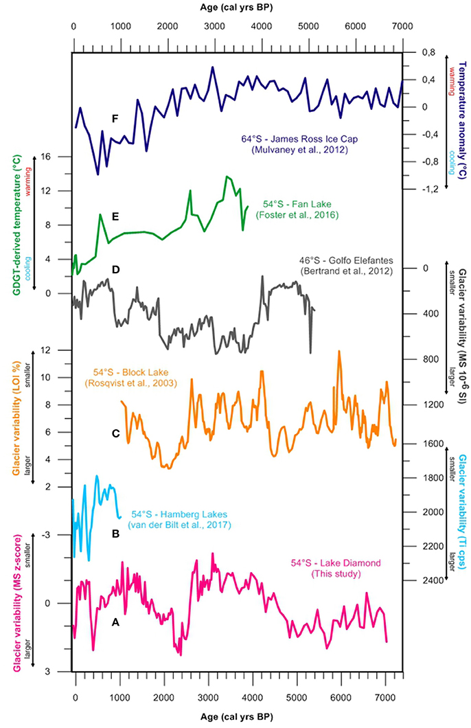
Figure 11. Comparison between our glacier reconstruction for Diamond glacier (A) and records of glacier variability on South Georgia from Block lake (Rosqvist and Schuber, 2003) (B) and Middle Hamberg lake (Van Der Bilt et al., 2017) (C), and Golfo Elefantes in Northern Patagonia (D) (Bertrand et al., 2012), a GDGT-derived temperature curve from Fan lake, Annenkov Island, South Georgia (E) (Foster et al., 2016), and δD-derived temperature anomalies relative to the 1961-1990 mean from James Ross Ice Cap, Antarctic Peninsula (F) (Mulvaney et al., 2012).

Glacier Retreat: 2000 ± 200 to 1000 ± 200 cal BP

Clay and silt dominate the sediments deposited in Diamond bog and Diamond lake between 2000 ± 200 cal BP and 1000 ± 200 cal BP clay (Unit F4, Figures 6A, Figure 11A). The decrease in relative sand content indicates lower runoff, and a gradual decrease in χbulk suggests glacier retreat back to mid-Holocene conditions (Figure 11A). This coincides with cirque glacier retreat in neighboring Husvik (Figure 2A), as demonstrated by Rosqvist and Schuber (2003) (Figure 11C) and higher temperatures at the western Antarctic Peninsula inferred from changes in peat growth (Yu et al., 2016).

Glacier Advance: 1000 ± 200 to 300 ± 100 cal BP

From 1000 ± 200 to 600 ± 100 cal BP there is a gradual increase in χbulk (Figure 11A), which we interpret as glacier advance based on the dominating clay and silt fractions in this interval. Between 500 ± 150 and 300 ± 100 cal BP, a sharp rise in χbulk and a higher concentration of sand and terrestrial plant fragments, suggests higher runoff. Peaking around 400 ± 150 cal BP, we interpret the increase in χbulk to represent the LIA. This glacier advance is also evident from the bog record, where a 4.5 cm thick silt layer with high χbulk values was deposited at 450 ± 200 cal BP. The LIA is also captured by Van Der Bilt et al. (2017) at 300 cal BP (Figures 11A,B) and widely documented on the island (e.g., Clapperton et al., 1978, 1989a,b; Gordon and Timmis, 1992; Roberts et al., 2010). Clapperton et al. (1989b) estimated an average ELA depression of 50 m during the LIA on the northeast coast of South Georgia. If applied to our site, the LIA moraine of Diamond glacier is likely represented by moraine M2 (Section Reconstructing the Glacier; Figure 2B). Coinciding with the LIA advance, Foster et al. (2016) document rapid cooling from c. 400 cal BP on Annenkov Island, and a millennial-scale cooling trend on James Ross Island culminates at c. 400 cal BP (Mulvaney et al., 2012) (Figures 11E,F).

Twentieth Century Glacier Advance

Increased χbulk suggests a recent glacier advance during the twentieth century. In the lake record, χbulk increases from AD 1920 ± 10 years, while a silt layer in the bog is dated to AD 1950 ± 10 years. Being a cirque glacier, we argue that Diamond glacier likely advanced in the 1930s, which is the case for cirque and small valley glaciers across the northeastern coast of South Georgia (Hayward, 1983; Gordon and Timmis, 1992; Gordon et al., 2008). The advance concurs with a drop in temperature to 3.3°C (AD 1931) at Grytviken compared to the mean summer temperature (Dec-Feb) of 4.9 ± 0.8°C (1905–2016), and is also recorded in Middle Hamberg lake (Van Der Bilt et al., 2017). According to Landsat imagery, Neumayer Glacier retreated 5600 m between 1999 and 2016 (Pelto, 2016), and we know from our field measurements that Diamond glacier front retreated approximately 150 m between 2008 and 2012. The glacier retreat is reflected in the lake sediments by decreasing χbulk (Figure 11A) in the topmost sediments, although not as clearly as in Van Der Bilt et al. (2017)'s record from Middle Hamberg lake (Figure 11C). Remobilization of paraglacial sediments in front of the rapidly retreating Diamond glacier, might mask the glacial signal in the lake and bog sediments during the paraglacial period, which typically lasts 10–50 years after a glacier retreat (Bakke et al., 2009). The ongoing glacier recession on South Georgia is well documented by observational data (Gordon et al., 2008; Cook et al., 2010) and follows a pattern of warming and glacier retreat observed from Patagonia to the Antarctic Peninsula (Koppes et al., 2015) as well as the rests of the world (Zemp et al., 2015).

Glacier Variability on South Georgia vs. Patagonia

The glacier reconstruction from Olsen Valley suggests that Diamond glacier was close to its maximum Holocene extent between 7200 ± 400 and 4800 ± 200 cal BP, 2700 ± 150 and 2000 ± 200 cal BP, 500 ± 150–300 ± 100 cal BP, and in the 1930s. Bertrand et al. (2012) provide a continuous glacier reconstruction from the Northern Patagonian Icefield based on a multiproxy analysis of a fjord sediment core, revealing repeated episodes of centennial scaled glacier advance over the past 5000 years (Figure 11D). The two records thus vary on a similar frequency and both show increased glacier activity during the last millennia. The glacier fluctuations documented by Bertrand et al. (2012) seem to be alternately in- and out of phase with those of Diamond glacier, although we find it too early to conclude about timing due to differing glacier response times and dating uncertainties. In general, the two records correspond best during periods of major glacier advance such as prior to 2000 cal BP, the LIA and the twentieth century advance, while they are out of phase on a millennial time scale during the mid-Holocene (Figures 11A,D). We speculate that the latitudinal expansion of the westerlies during cold phases causes both sites to be influenced by the same wind circulation system (Lamy et al., 2010), improving the correspondence of the glacier records during these periods. There are also other records from Patagonia to compare with. It turns out that the timing of South Georgia glacier advances concur with several of the Holocene glaciations of the Patagonian Icefield suggested by Anyia (2013) and Strelin et al. (2014), particularly since c. 2700 cal BP. Anyia (2013) proposes five Neoglacial episodes: at 4500–4000 cal BP, 3600–3300 cal BP, 2700–2000 cal BP, 1600–900 cal BP and in the seventeenth to nineteenth centuries century. Based on surface exposure dating, Strelin et al. (2014) suggest six Holocene glacier advances of the Southern Patagonian Icefield at 7700–7200 cal BP, 6000–5000 cal BP, 2500–2000 cal BP, 1500–1100 cal BP >400 cal BP and <300 cal BP. The covariance between South Georgia and Patagonian glacier fluctuations on centennial time scales points to shared regional climate forcing, possibly related to persistent changes in the Southern Hemisphere westerlies which arguably can have a large impact on local variations in precipitation and temperature (cf. Moreno et al., 2014).

Conclusions

A 7000-year long continuous cirque glacier reconstruction, based on analyses of glacier-fed lake and bog sediments from the same catchment, suggest that glaciers on South Georgia have varied on centennial time scales for the time interval in question. Evidence for this pattern of variability is obtained by employing the same combination of magnetic, physical, and geochemical sedimentary analyses on the two independently dated sediment archives from the bog and lake, which in sum have enabled us to reproduce the history of the cirque glacier and precisely constrain the timing of the glacier fluctuations. A set of marginal moraines in the catchment outline the past extent of the Neumayer tidewater glacier, which probably filled the lower valley during the Late-Pleistocene, and subsequently advanced to a position just west of Olsen Valley several times, including the past century. In front of the cirque glacier, a mapped moraine sequence provide spatial constraints to the continuous glacier reconstruction. Reconstructed ELAs demonstrate that the recent glacier retreat stands out in a Holocene context although changes are within 100 m altitude. Based on the combination of two different glacial sedimentary archives, a consistent picture emerges of the Holocene glacier evolution in the studied catchment; characterized by deglaciation some time prior to 9900 ± 250 cal BP, and glacier advance close to its maximum Holocene extent between 7200 ± 400 and 4800 ± 200 cal BP, 2700 ± 150 and 2000 ± 200 cal BP, 500 ± 150–300 ± 100 cal BP, and in the 1930s. Changes in glacier size is constrained by a sequence of moraines in front of the cirque glacier. The reconstructed glacier fluctuations agrees with existing moraine chronologies, two previous continuous glacier reconstructions and various paleoclimate records on South Georgia, highlighting the ability of these sedimentary records to capture concordant shifts. Moreover, the centennial scaled glacier variability documented here are largely in-phase with patterns of retreat and advance of Patagonian glaciers, especially during the past three millennia, although caution is warrant due to chronological uncertainties. This, nevertheless, points to large-scale climate shifts potentially linked to the Southern Hemisphere Westerlies, although this is something that requires further studies before any solid conclusions can be drawn.

Author Contributions

JB, ØP, and LO were responsible for the conceptual design of the work. JB and ØP mapped and the study area in 2008, and JB and colleagues further mapped the catchment and cored the lake and bog in 2012. LO performed the laboratory analyses, and lead the writing and compilation of figures and tables. All authors have given substantial contributions to the interpretations of the data and the writing of the article. In cooperation with LO and JW performed the age-depth modeling and statistical cross-matching (Figures 7–8), and WvdB designed the maps (Figures 1–3). All authors approve of the submitted version of the manuscript and thereby agree to be accountable for all aspects of the work, ensuring that questions related to the accuracy or integrity of any part of the work are appropriately investigated and resolved.

Conflict of Interest Statement

The authors declare that the research was conducted in the absence of any commercial or financial relationships that could be construed as a potential conflict of interest.

Acknowledgments

This is a contribution from the project “Shifting Climate States of the Polar Regions,” funded by the Norwegian Research Council (Grant 210004). We would like to thank Anne Bjune, Bjørn Christian Kvisvik, Åsmund Bakke, Sunniva Solheim Vatle, and Thom Whitfield for their effort during fieldwork, and British Antarctic Survey for their field support. We would also like to thank Sven Lukas and Gunhild Rosqvist for contributing to the manuscript, and Lubna S. J. Al-Saadi and Eivind W. N. Støren for help with grain size measurements. Finally, thank you to reviewers Olga N. Solomina and Bethan J. Davies, whose comments helped improve and clearify the manuscript.

Supplementary Material

The Supplementary Material for this article can be found online at: https://www.frontiersin.org/articles/10.3389/feart.2018.00002/full#supplementary-material

Footnotes

1. ^Google (n.d.). Google Map of South Georgia [Online]. Available online at: https://goo.gl/Dr1pYP (Accessed 2008).

References

Anyia, M. (2013). Holocene glaciations of Hielo Patagónico (Patagonian Icefield), South America: a brief review. Geochem. J. 47, 98–105. doi: 10.2343/geochemj.1.0171

CrossRef Full Text

Bakke, J., Dahl, S. O., Paasche, Ø., Simonsen, J. R., Kvisvik, B., Bakke, K., et al. (2010). A complete record of Holocene glacier variability at Austre Okstindbreen, northern Norway: an integrated approach. Quat. Sci. Rev. 29, 1246–1262. doi: 10.1016/j.quascirev.2010.02.012

CrossRef Full Text | Google Scholar

Bakke, J., Lie, Ø., Heegaard, E., Dokken, T., Haug, G. H., Birks, H. J. B., et al. (2009). Rapid oceanic and atmospheric changes during the Younger Dryas cold period. Nat. Geosci. 2, 202–205. doi: 10.1038/ngeo439

CrossRef Full Text | Google Scholar

Bakke, J., Lie, Ø., Nesje, A., Dahl, S. O., and Paasche, Ø. (2005). Utilizing physical sediment variability in glacier-fed lakes for continuous glacier reconstructions during the Holocene, northern Folgefonna, western Norway Holocene 15, 161–176. doi: 10.1191/0959683605hl797rp

CrossRef Full Text | Google Scholar

Bakke, J., and Paasche, Ø. (2011). “Sediment core and glacial environment reconstruction,” in Encyclopedia of Snow, Ice and Glaciers, eds V. P. Singh, P. Singh, and U. K. Haritashya (Dordrecht: Springer).

Google Scholar

Balco, G. (2009). The geographic footprint of glacier change. Science 324, 599–600. doi: 10.1126/science.1172468

PubMed Abstract | CrossRef Full Text | Google Scholar

Ballantyne, C. K. (1989). The loch lomond readvance on the isle of skye, scotland: glacier reconstruction and paleoclimatic implications. J. Quatern. Sci. 4, 9–108. doi: 10.1002/jqs.3390040201

CrossRef Full Text | Google Scholar

Ballantyne, C. K. (2002). Paraglacial geomorphology. Quat. Sci. Rev. 21, 1935–2017. doi: 10.1016/S0277-3791(02)00005-7

CrossRef Full Text | Google Scholar

Bentley, M. J., Evans, D. J. A., Fogwill, C. J., Hansom, J. D., Sugden, D. E., and Kubik, P. W. (2007). Glacial geomorphology and chronology of deglaciation, South Georgia, sub-Antarctic. Quat. Sci. Rev. 26, 644–677. doi: 10.1016/j.quascirev.2006.11.019

CrossRef Full Text | Google Scholar

Bertrand, S., Hughen, K. A., Lamy, F., Stuut, J.-B. W., Torrejón, F., and Lange, C. B. (2012). Precipitation as the main driver of Neoglacial fluctuations of Gualas glacier, Northern Patagonian Icefield. Clim. Past 8, 1–16. doi: 10.5194/cp-8-1-2012

CrossRef Full Text | Google Scholar

Björck, S., Håkansson, H., Olsson, S., Barnekow, L., and Janssens, J. (1993). Paleoclimatic studies in South Shetland Islands, Antarctica, based on numerous stratigraphic variables in lake sediments. J. Paleolimnol. 8, 233–272. doi: 10.1007/BF00177858

CrossRef Full Text | Google Scholar

Björck, S., Håkansson, H., Zale, R., Karlén, W., and Jönsson, B. L. (1991). A late Holocene lake sediment sequence from Livingstone Island, South Shetland Islands, with paleoclimatic implications. Antarct. Sci. 3, 61–72. doi: 10.1017/S095410209100010X

CrossRef Full Text | Google Scholar

Blaauw, M. (2010). Methods and code for “classical” age-modelling of radiocarbon sequences. Quat. Geochronol. 5, 512–518. doi: 10.1016/j.quageo.2010.01.002

CrossRef Full Text | Google Scholar

Böning, C. W., Dispert, A., Visbeck, M., Rintoul, S. R., and Schwarzkopf, F. U. (2008). The response of the Antarctic Circumpolar Current to recent climate change. Nat. Geosci. 1, 864–869. doi: 10.1038/ngeo362

CrossRef Full Text | Google Scholar

Clapperton, C. M., Sugden, D. E., Birnie, J., and Wilson, M. (1989a). Late-glacial and Holocene glacier fluctuations and environmental change on South Georgia, Southern Ocean. Quatern. Res. 31, 210–228. doi: 10.1016/0033-5894(89)90006-9

CrossRef Full Text | Google Scholar

Clapperton, C. M., Sugden, D. E., Birnie, R. V., Hanson, J. D., and Thom, G. (1978). “Glacier fluctuations in South Georgia and comparison with other island groups in the Scotia Sea,” in Antarctic Glacial History and World Palaeoenvironments, ed E. M. Van Zinderen Bakker (Rotterdam: A. A. Balkema), 99–104.

Clapperton, C. M., Sugden, D. E., and Pelto, M. (1989b). “Relationship of land terminating and fjord glaciers to Holocene climatic change, South Georgia, Antarctica,” in Glacier Fluctuations and Climatic Change, ed J. Oerlemans (Dordrecht: Kluwer Academic Publishers), 57–75.

Google Scholar

Cook, A. J., Poincet, S., Cooper, A. P. R., Herbert, D. J., and Christie, D. (2010). Glacier retreat on South Georgia and implications for the spread of rats. Antarct. Sci. 22, 255–263. doi: 10.1017/S0954102010000064

CrossRef Full Text | Google Scholar

Davies, S., Lamb, H., and Roberts, S. (2015). “Micro-XRF core scanner in palaeolimnology: recent developments,” in Micro-XRF Studies of Sediment Cores. Developments in Paleoenvironmental Research, eds I. Croudace and R. Rothwell. (Dordrecht: Springer), 189–226.

Google Scholar

Dean, W. E. Jr. (1974). Determination of carbonate and organic matter in calcareous sediments and sedimentary rocks by loss on ignition: comparison with other methods. J. Sediment. Petrol. 44, 242–248.

Google Scholar

Foster, L. C., Pearson, E. J., Juggins, S., Hodgson, D., Saunders, K. M., Verleyen, E., et al. (2016). Development of a regional glycerol dialkyl tetraether (GDGT)-temperature calibration for Antarctic and sub-Antarctic lakes. Earth Planet. Sci. Lett. 433, 370–379. doi: 10.1016/j.epsl.2015.11.018

CrossRef Full Text | Google Scholar

Gille, S. T. (2002). Warming of the Southern Ocean since the 1950s. Science 295, 1275–1277. doi: 10.1126/science.1065863

PubMed Abstract | CrossRef Full Text | Google Scholar

Gille, S. T. (2008). Decadal-scale temperature trends in the Southern Hemisphere Ocean. J. Clim. 21, 4749–4765. doi: 10.1175/2008JCLI2131.1

CrossRef Full Text | Google Scholar

Gordon, J. E., Haynes, V. M., and Hubbard, A. (2008). Recent glacier changes and climate trends on South Georgia. Glob. Planet Change 60, 72–84. doi: 10.1016/j.gloplacha.2006.07.037

CrossRef Full Text | Google Scholar

Gordon, J. E., and Timmis, R. J. (1992). Glacier fluctuations on South Georgia during the 1970s and early 1980s. Antarct. Sci. 4, 215–226. doi: 10.1017/S0954102092000336

CrossRef Full Text | Google Scholar

Graham, A. G., Kuhn, G., Meisel, O., Hillenbrand, C.-D., Hodgson, D. A., Ehrmann, W., et al. (2017). Major advance of South Georgia glaciers during the Antarctic Cold Reversal following extensive sub-Antarctic glaciation. Nat. Commun. 8:14798. doi: 10.1038/ncomms14798

PubMed Abstract | CrossRef Full Text | Google Scholar

Grosjean, M., Geyh, M. A., Messerli, B., Schreier, H., and Veit, H. (1998). A late-Holocene (<2600 BP) glacial advance in the south-central Andes (29°), northern Chile. Holocene 8, 473–479. doi: 10.1191/095968398677627864

CrossRef Full Text | Google Scholar

Hayward, R. J. C. (1983). Glacier fluctuations in South Georgia, 1883-1974. Br. Antarct. Surv. Bull. 52, 47–61.

Herman, F., Beyssac, O., Brughelli, M., Lane, S. N., Leprince, S., Adatte, T., et al. (2015). Erosion by an Alpine glacier. Science 350, 193–195. doi: 10.1126/science.aab2386

PubMed Abstract | CrossRef Full Text | Google Scholar

Hodgson, D. A., Graham, A. G. C., Griffiths, H. J., Roberts, S. J., Cofaigh, C. Ó., Bentley, M. J., et al. (2014). Glacial history of sub-Antarctic South Georgia based on the submarine geomorphology of its fjord. Quat. Sci. Rev. 89, 129–147. doi: 10.1016/j.quascirev.2013.12.005

CrossRef Full Text | Google Scholar

Hodgson, D. A., and Sime, L. S. (2010). Southern westerlies and CO₂. Nat. Geosci. 3, 666–667. doi: 10.1038/ngeo970

CrossRef Full Text | Google Scholar

Hogg, A. G., Hua, Q., Blackwell, P. G., Niu, M., Buck, C. E., Guilderson, T. P., et al. (2013). SHCal13 southern hemisphere calibration, 0-55,000 years cal BP. Radiocarbon 55, 1889–1903. doi: 10.2458/azu_js_rc.55.16783

CrossRef Full Text | Google Scholar

Hua, Q., Barbetti, M., and Rakowski, A. Z. (2013). Atmospheric radiocarbon for the period 1950-2010. Radiocarbon 55, 2059–2072. doi: 10.2458/azu_js_rc.v55i2.16177

CrossRef Full Text | Google Scholar

Karlén, W. (1976). Lacustrine sediments and tree-limit variations as indicators of holocene climatic fluctuations in lappland, Northern Sweden. Geogr. Ann. Ser. A 58, 1–34. doi: 10.2307/520740

CrossRef Full Text | Google Scholar

Karlén, W. (1981). Lacustrine sediment studies. A technique to obtain a continuous record of Holocene glacier variations. Geogr. Ann. Ser. A 63, 273–281. doi: 10.2307/520840

CrossRef Full Text | Google Scholar

Koppes, M., Hallet, B., Rignot, E., Mouginot, J., Wellner, J. S., and Boldt, K. (2015). Observed latitudinal variations in erosion as a function of glacier dynamics. Nature 526, 100–103. doi: 10.1038/nature15385

PubMed Abstract | CrossRef Full Text | Google Scholar

Kylander, M. E., Ampel, L., Wohlfarth, B., and Veres, D. (2011). High-resolution X-ray fluorescence core scanning analysis of Les Echets (France) sedimentary sequence: new insights from chemical proxies. J. Quatern. Sci. 26, 109–117. doi: 10.1002/jqs.1438

CrossRef Full Text | Google Scholar

Lamy, F., Killian, R., Arz, H. W., Francois, J. P., Kaiser, J., Prange, M., et al. (2010). Holocene changes in the position and intensity of the southern westerly wind belt. Nat. Geosci. 3, 695–699. doi: 10.1038/ngeo959

CrossRef Full Text | Google Scholar

Lanci, L., and Lowrie, W. (1997). Magnetostratigraphic evidencethat “tiny wiggles” in the oceanic magnetic anomaly record represent geomagnetic paleointensity variations. Earth Planet. Sci. Lett. 148, 581–592. doi: 10.1016/S0012-821X(97)00055-1

CrossRef Full Text | Google Scholar

Lenton, A., and Matear, R. J. (2007). Role of the Southern Annular Mode (SAM) in Southern Ocean CO₂ uptake. Glob. Biogeochem. Cycles 21, 1–17. doi: 10.1029/2006GB002714

CrossRef Full Text | Google Scholar

Le Quéré, C., Rödenbeck, C., Buitenhuis, E. T., Conway, T. J., Langenfelds, R., Gomez, A., et al. (2007). Saturation of the Southern Ocean CO₂ sink due to recent climate change. Science 316, 1735–1738. doi: 10.1126/science.1136188

PubMed Abstract | CrossRef Full Text | Google Scholar

Lukas, S. (2012). Processes of annual moraine formation at a temperate alpine valley glacier: insights into glacier dynamics and climatic controls. Boreas 41, 463–480. doi: 10.1111/j.1502-3885.2011.00241.x

CrossRef Full Text | Google Scholar

Matthews, J. A., Berrisford, M. S., Dresser, P. Q., Nesje, A., Dahl, S. O., Bjune, A. E., et al. (2005). Holocene glacier history of Bjørnbreen and climatic reconstruction in central Jotunheimen, Norway, based on proximal glaciofluvial stream-bank mires. Quat. Sci. Rev. 24, 67–90. doi: 10.1016/j.quascirev.2004.07.003

CrossRef Full Text | Google Scholar

Matthews, J. A., and Karlén, W. (1992). Asynchronous neoglaciation and Holocene climatic change reconstructed from Norwegian glaciolacustrine sedimentary sequences. Geology 20, 991–994. doi: 10.1130/0091-7613(1992)020<0991:ANAHCC>2.3.CO2

CrossRef Full Text | Google Scholar

Moreno, P. I., Vilanova, I., Villa-Martínez, R., Garreaud, R. D., Rojas, M., and De Pol-Holz, R. (2014). Southern Annular Mode-like changes in southwestern Patagonia at centennial timescales over the last three millennia. Nat. Commun. 5:4375. doi: 10.1038/ncomms5375

PubMed Abstract | CrossRef Full Text | Google Scholar

Mulvaney, R., Abram, N. J., Hindmarsh, R. C., Arrowsmith, C., Fleet, L., and Triest, J. (2012). Recent Antarctic peninsula warming relative to Holocene climate and ice-shelf history. Nature 489, 141–144. doi: 10.1038/nature11391

PubMed Abstract | CrossRef Full Text | Google Scholar

Oerlemans, J. (2005). Extracting a climate signal from 169 Glacier records. Science 308, 675–677. doi: 10.1126/science.1107046

PubMed Abstract | CrossRef Full Text | Google Scholar

Orsi, A. H., Whitworth, T., and Nowlin, W. D. (1995). On the meridional extent and fronts of the Antarctic Circumpolar Current. Deep Sea Res. Part I 42, 641–673. doi: 10.1016/0967-0637(95)00021-W

CrossRef Full Text | Google Scholar

Osmaston, H. (2005). Estimates of glacier equilibrium line altitudes by the Area x Altitude, the Area x Altitude Balance Ratio and the Area x Altitude Balance Index methods and their validation. Quatern. Int. 138–139, 22–31. doi: 10.1016/j.quaint.2005.02.004

CrossRef Full Text

Østrem, G., Dale Selvig, K., and Tandberg, K. (1988). Atlas of Glaciers in South Norway. Oslo: Noregs vassdrags- og energidirektorat.

Paasche, Ø., Dahl, S. O., Bakke, J., Løvlie, R., and Nesje, A. (2007). Cirque glacier activity in arctic Norway during the last deglaciation. Quatern. Res. 68, 387–399. doi: 10.1016/j.yqres.2007.07.006

CrossRef Full Text | Google Scholar

Pelto, M. (2016). Neumayer Glacier, South Georgia, 5.6 km retreat 1999-2016 [Online]. From a Glacier's perspective. Available online at: https://goo.gl/rRuYBb (Accessed September 8, 2017).

Pendlebury, S. F., and Barnes-Keoghan, I. P. (2007). Climate and climate change in the sub-Antarctic. Pap. Proc. R. Soc. Tasmania 141, 67–81.

Google Scholar

Porter, S. (1975). Equilibrium-line altitudes of late Quaternary glaciers in the Southern Alps, New Zealand. Quatern. Res. 5, 27–47. doi: 10.1016/0033-5894(75)90047-2

CrossRef Full Text | Google Scholar

Quilty, P. G. (2007). Origin and evolution of the sub-Antarctic islands: the foundation. Pap. Proc. R. Soc. Tasmania 141, 35–58.

Google Scholar

Renberg, I., and Hansson, H. (2008). The HTH sediment corer. J. Paleolimnol. 40, 655–659 doi: 10.1007/s10933-007-9188-9

CrossRef Full Text | Google Scholar

Roberts, S. J., Hodgson, D. A., Shelley, S., Royles, J., Griffiths, H. J., Deen, T. J., et al. (2010). Establishing lichonometric ages for nineteenth- and twentieth-century glacier fluctuations on South Georgia (South Atlantic). Geogr. Ann. Ser. A 92, 125–139. doi: 10.1111/j.1468-0459.2010.00382.x

CrossRef Full Text | Google Scholar

Rosqvist, G. C., and Schuber, P. (2003). Millennial-scale climate changes on South Georgia, Southern Ocean. Quatern. Res. 59, 470–475. doi: 10.1016/S0033-5894(03)00036-X

CrossRef Full Text | Google Scholar

Rubensdotter, L., and Rosqvist, G. (2005). Influcence of geomorphological setting, fluvial-, glaciofluvial- and mass-movement processes on sedimentation in alpine lakes. Holocene 19, 665–678. doi: 10.1177/0959683609104042

CrossRef Full Text

Scambos, T. A., Berthier, E., Haran, T., Schuman, C. A., Cook, A. J., Ligtenberg, S., et al. (2014). Detailed ice loss pattern in the northen Antarctic Peninsula: widespread decline driven by ice front retreats. Cryosphere 8, 2135–2145. doi: 10.5194/tc-8-2135-2014

CrossRef Full Text | Google Scholar

Scar (2015). Antarctic Digital Database, Version 6.0. Database, Manual and Bibliography [Online]. Available online at: http://www.add.scar.org/ (Accessed 2017).

SGGIS (2017). South Georgia Geographic Information Systems [Online]. Available online at: http://sggis.gov.gs/ (Accessed 2017).

Sigman, D. M., Hain, M. P., and Haug, G. H. (2010). The polar ocean and glacial cycles in atmospheric CO₂ concentration. Nature 466, 47–55. doi: 10.1038/nature09149

CrossRef Full Text | Google Scholar

Smith, R. I. L. (1981). Types of peat and peat-forming vegetation on South Georgia. Br. Antarct. Survey Bull. 53, 119–139.

Solomina, O. N., Bradley, R. S., Hodgson, D. A., Ivy-Ochs, S., Jomelli, V., Mackintosh, A. N., et al. (2015). Holocene glacier fluctuations. Quat. Sci. Rev. 111, 9–34. doi: 10.1016/j.quascirev.2014.11.018

CrossRef Full Text | Google Scholar

Sterken, M., Roberts, S., Hodgson, D. A., Vyverman, W., Balbo, A. L., Sabbe, K., et al. (2012). Holocene glacial and climate history of Prince Gustav Channel, northeastern Antarctic Peninsula. Quat. Sci. Rev. 31, 93–111. doi: 10.1016/j.quascirev.2011.10.017

CrossRef Full Text | Google Scholar

Strelin, J. A., Kaplan, M. R., Vandergoes, M. J., Denton, G. H., and Schaefer, J. M. (2014). Holocene glacier history of the Lago Argentino basin, Southern Patagonian Icefield. Quat. Sci. Rev. 101, 124–145. doi: 10.1016/j.quascirev.2014.06.026

CrossRef Full Text | Google Scholar

Strother, S. L., Salzmann, U., Roberts, S. J., Hodgson, D. A., Woodward, J., Van Nieuwenhuyze, W., et al. (2015). Changes in Holocene climate and the intensity of Southern Hemisphere Westerly Winds based on a high-resolution palynological record from sub-Antarctic South Georgia. Holocene 25, 263–279. doi: 10.1177/0959683614557576

CrossRef Full Text | Google Scholar

Tanner, P. W. G. (1981). “Turbidite sequences on South Georgia, South Atlantic: their structural relationship and provencance,” in Geological Evolution of Antarctica, eds M. R. A. Thomson, L. A. Crame, and J. W. Thomson (Cambridge: Cambridge University Press), 353–359.

Thompson, R., Batterbee, R. W., O'sullivan, P. E., and Oldfield, F. (1975). Magnetic susceptibility of lake sediments. Limnol. Oceanogr. 20, 687–698. doi: 10.4319/lo.1975.20.5.0687

CrossRef Full Text | Google Scholar

Thompson, R., and Oldfield, F. (1986). Environmental Magnetism. London: Allen and Unwin.

Google Scholar

Thompson, D. W. J., Solomon, S., Kushner, P. J., England, M. H., Grise, K. M., and Karoly, D. J. (2011). Signatures of the Antarctic ozone hole in Southern Hemisphere surface climate change. Nat. Geosci. 4, 741–749. doi: 10.1038/ngeo1296

CrossRef Full Text | Google Scholar

Van Der Bilt, W. G. M., Bakke, J., Werner, J. P., Paasche, Ø., Rosqvist, G., and Vatle, S. S. (2017). Late Holocene glacier reconstruction reveals retreat behind present limits and two-stage Little Ice Age on subantarctic South Georgia. J. Quatern. Sci. 32, 888–901. doi: 10.1002/jqs.2937

CrossRef Full Text | Google Scholar

Van Der Putten, N., Stieperaere, H., Verbruggen, C., and Ochyra, R. (2004). Holocene paleoecology and climate history of South Georgia (sub-Antarctica) based on macrofossil record of bryophytes and seeds. Holocene 14, 382–392. doi: 10.1191/0959683604hl714rp

CrossRef Full Text | Google Scholar

Van Der Putten, N., and Verbruggen, C. (2005). The onset of deglaciation of Cumberland Bay and Stromness Bay, South Georgia. Antarct. Sci. 17, 29–32. doi: 10.1017/S0954102005002397

CrossRef Full Text | Google Scholar

Van Der Putten, N., Verbruggen, C., Ochyra, R., Spassov, S., De Beaulieu, J.-L., De Dapper, M., et al. (2009). Peat bank growth, Holocene paleoecology climate history of South Georgia (sub-Antarctica), based on a botanical macrofossil record. Quat. Sci. Rev. 28, 65–79. doi: 10.1016/j.quascirev.2008.09.023

CrossRef Full Text | Google Scholar

Vasskog, K., Kvisvik, B. C., and Paasche, Ø. (2016). Effects of hydrogen peroxide treatment on measurements of lake sediment grain-size distribution. J. Paleolimnol. 56, 365–381. doi: 10.1007/s10933-016-9924-0

CrossRef Full Text | Google Scholar

Vasskog, K., Paasche, Ø., Nesje, A., Boyle, J. F., and Birks, H. J. B. (2012). A new approach for reconstructing glacier variability based on lake sediments recording input from more than one glacier. Quatern. Res. 77, 192–204. doi: 10.1016/j.yqres.2011.10.001

CrossRef Full Text | Google Scholar

Vaughan, D. G., Marshall, G. J., Connelley, W. M., Parkinson, C., Mulvaney, R., Hodgson, D. A., et al. (2003). Recent rapid regional climate warming on the Antarctic Peninsula. Clim. Change 60, 243–274. doi: 10.1023/A:1026021217991

CrossRef Full Text | Google Scholar

Wang, G., and Cai, W. (2013). Climate-change impact on the 20th-century relationship between the Southern Annular Mode and global mean temperature. Sci. Rep. 3, 1–6. doi: 10.1038/srep02039

PubMed Abstract | CrossRef Full Text | Google Scholar

Weidick, A. (1992). Glacier Inventory and Atlas of West Greenland. Copenhagen: Gronland Geologiske Undersøgelse.

Google Scholar

Werner, J. P., and Tingley, M. P. (2015). Technical note: probabilistically constraining proxy age-depth models within a Bayesian hierarchical reconstruction model. Clim. Past 11, 533–545. doi: 10.5194/cp-11-533-2015

CrossRef Full Text | Google Scholar

Yu, Z., Beilman, D. W., and Loisel, J. (2016). Transformations of landscape and peat-forming ecosystems in response to late Holocene climate change in the western Antarctic Peninsula. Geophys. Res. Lett. 43, 7186–7195. doi: 10.1002/2016GL069380

CrossRef Full Text | Google Scholar

Yuan, X. J. (2004). ENSO-related impacts on Antarctic sea ice: a synthesis of phenomenon and mechanisms. Antarct. Sci. 16, 415–425. doi: 10.1017/S0954102004002238

CrossRef Full Text | Google Scholar

Zemp, M., Frey, H., Gärtner-Roer, I., Nussbaumer, S. U., Hoelzle, M., Frank, P., et al. (2015). Historically unprecedented global glacier decline in the early 21st century. J. Glaciol. 61, 745–762. doi: 10.3189/2015JoG15J017

CrossRef Full Text | Google Scholar