Spatial Variability in Patterns of Glacier Change across the Manaslu Range, Central Himalaya

Introduction

High Mountain Asia contains the largest concentration of glacier ice outside of the polar areas. Glacial meltwater has many implications for the regional population such as irrigation and hydroelectric power production (Immerzeel et al., 2010; Bolch et al., 2012), as well as hazards such as glacial lake outburst floods (GLOFs) that have killed more than 6,300 people in Central Asia since the 1500s (Richardson and Reynolds, 2000; Bolch et al., 2008; Schwanghart et al., 2014; Carrivick and Tweed, 2016).

Existing in-situ glacier mass balance data in the Himalayas is extremely limited and biased toward accessible small to medium sized and debris-free glaciers (Bolch et al., 2012; Gardelle et al., 2013). A high level of uncertainty therefore exists when interpreting regional trends in Himalayan glaciers based on in-situ data. Remote sensing data allows systematic monitoring of glaciers over decadal scales. Within the Himalayas, remote sensing has permitted large scale investigations of glacier area (Bajracharya et al., 2014; Nuimura et al., 2014; Robson et al., 2015), glacier velocities (Copland et al., 2009; Heid and Kääb, 2012b; Dehecq et al., 2015), and geodetic mass balances (Bolch et al., 2011; Gardelle et al., 2012b; Kääb et al., 2012; Maurer and Rupper, 2015; Neckel et al., 2017). Landsat imagery has been used to establish that the Nepali Himalayas contain a total of 3808 glaciers with a total area of 3902 km² as of 2010 (Bajracharya, 2014). Within Nepal, Digital Elevation Model (DEM) differencing has been used to calculate surface elevation changes and geodetic mass balances back to the 1960s and 1970s using declassified Corona imagery within predominantly two Nepali glacier regions, namely the Everest Region in Eastern Nepal (Bolch et al., 2011; King et al., 2017), and the Langtang valley in Central Nepal (Pellicciotti et al., 2015; Ragettli et al., 2016). Additionally the Nepali Himalayas have seen some pioneering studies on ice-cliffs and supraglacial ponds on debris-covered glaciers, with ice cliffs found to ablate by between six and 10 times the mean glacier ablation rate (Immerzeel et al., 2014; Brun et al., 2016) and contribute up to 20% of the total glacier ablation (Sakai et al., 2000).

Himalayan glacier change has been found to be heterogeneous and vary profusely from one region to another (Scherler et al., 2011; Kääb et al., 2012, 2015). This in part reflects the heterogeneous and varying climate across the Himalayas as well as the presence of supraglacial debris in some regions. The Himalayan glaciers are influenced by three major precipitation regimes (Indian Summer Monsoon, Mid-Latitude Westerlies, South East Asian Monsoon) and their strength and the timing (summer or winter) vary from region to region (Ageta and Higuchi, 1984; Benn and Lehmkuhl, 2000; Owen and Benn, 2005). The rugged topography of the Himalayas causes significant local and regional variations in climate (Owen and Benn, 2005).

Many Himalayan glaciers are covered by supraglacial debris. The presence of supraglacial debris allows for glacier tongues to extend to much lower-lying elevations than would otherwise be possible (Owen and Benn, 2005). The effects of debris-cover on glacier mass balance are poorly known, and can act to either retard or exacerbate glacier melting depending on debris thickness, composition, and distribution (Reznichenko et al., 2010; Zhang et al., 2011). Many studies have reported thresholds of debris-thickness, above which the debris acts to insulate the glacier as opposed to amplifying melt rates (Reznichenko et al., 2010). These thresholds however do not consider the importance of supraglacial lakes and ice cliffs on the mass balance of debris-covered glaciers that has been highlighted by many scientific papers (Immerzeel et al., 2014; Juen et al., 2014; Watson et al., 2017). In many cases terminus positions of debris-covered glaciers in the Himalayas have remained in the same position over the previous decades despite glacier down-wasting and mass loss (Scherler et al., 2011; Benn et al., 2012; Nagai et al., 2013).

Objectives

The objectives of this paper are to investigate decadal scale glacier area, geodetic mass balance, and velocity changes in the Manaslu region of Nepal, a previously undocumented region in the Himalayas. Using the combination of our satellite derived glacier change parameters, we aim to better understand glacier changes in this region over the past decades. Our study addresses how the glaciers in this region vary spatially and temporally. By putting our results in the context of other regions of the Nepali Himalayas, we help resolve how the Himalayan cryosphere is changing over a broader scale.

Study Area

Our study interest is the glaciers in the Manaslu region of the Central Nepali Himalayas (Figure 1), ~230 km west of Mount Everest. The glacier changes of this region are yet to be extensively addressed in the literature. The Manaslu region contains an assortment of clean, debris-covered, and stagnant ice. We restricted our analysis to the glaciers centered around the mountains Baudha, Manaslu, Himlung, Ratna Chuli, and Lugula (Figure 1). The SRTM (Shuttle Radar Topography Mission) DEM is not complete over the entire area due to rugged topography. We therefore focused our study on 41 glaciers (~500 km² ice) that were mostly covered by the SRTM DEM. The Manaslu region covers ~2250 km² of which 30% is covered by glaciers. Our study area extends across the Nepali-Tibetan border, which is also the mountain divide between the humid, monsoon-driven Himalayas, and the arid Tibetan plateau (Benn and Owen, 1998; Maussion et al., 2014). While the glaciers north of the topographic divide are predominantly clean glaciers, the majority of those south of the divide are covered by supraglacial debris in their ablation areas. This difference in debris-cover is partly attributed to the larger debris supply area on the southern side of the mountains, as well as stronger diurnal freeze-thaw cycles found south of the topographic divide, where winter temperatures fluctuate more around freezing point (Nagai et al., 2013).

FIGURE 1

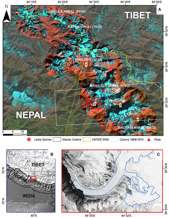
Figure 1. (A) Location of the glaciers studied (outlines derived from Robson et al., 2015) within the Manaslu Region (28°N, 84°E), and (B) the location of the Manaslu Region within Nepal. Thulagi Glacier (C) previously terminated in Dona Lake (shown on the 1970 Corona image). Larke Samdo weather station is shown as a red diamond outline. Four glaciers that are referred to in the text in more detail are shown on (A): 1—Ponkar Glacier, 2—Thulagi Glacier, 3—Hinang Glacier, 4—Himal Chuli Glacier. All the glaciers within the emphasized image on (A) were covered by the SETSM and SRTM DEMs. The coverage of the ASTER and Corona datasets are shown in orange and gray in (A). The boundary between the northern group of glaciers and the southern group of glaciers is shown as a yellow dashed line. Background image: Landsat 8 (26th December 2013). Hillshade in (C) is from naturalearthdata.com.

The glaciers in the study area are typically 0.5–1 km in width and 5–15 km in length with areas that vary from 5.6 to 32.0 km². Debris-covered glaciers in the south range in elevation from 3500 to over 7000 m a.s.l, while clean ice glaciers in Tibet are found in elevations above 5500 m a.s.l. Larke Samdo weather station (84°38E, 28°39N, 3650 m a.s.l; Figure 1) recorded monthly mean temperatures between 26.7 and 12.8°C and a mean precipitation of ~1000 mm a year (Department of Hydrology and Meteorology, Department of Hydrology Meteorology (Government Of Nepal)., 2014). The central Himalayas receive 80% of annual precipitation during the summer monsoon (July to September) when rates of glacier accumulation and ablation are simultaneously at their highest (Ageta and Higuchi, 1984; Benn and Owen, 1998). The glaciers situated on the Tibetan Plateau receive less precipitation and as such respond primarily to variations in the ablation season temperature (Owen and Benn, 2005).

Some glaciers are discussed in more detail in the text. Thulagi Glacier (GLIMS ID: G084538E28524N) is ~27 km² in size and extends from ~4100 to 7500 m a.s.l. As Thulagi Glacier has melted, Dona Lake, a moraine-dammed lake situated at the glacier terminus, has grown and is now 0.9 km² in size. Pant and Reynolds (2000) found that the moraine-dam contained large amounts of dead ice. Mass movements in the valley, calving events from the glacier, or downwasting of the moraine dam could potentially cause a breach of the ice cored moraine and a GLOF (Richardson and Reynolds, 2000). Dona Lake has been identified as a potentially dangerous glacial lake in the Himalayas (Mool, 2011; Rounce et al., 2017). Ponkar Glacier (GLIMS ID G084459E28695N) flows south out of Himlung and has a sizable accumulation area and a high glacier velocity. We also focused on Hinang Glacier (G084640E28489N), and Himal Chuli (G084759E28427N) Glaciers, both of which flow south east from Manaslu and Baudha, respectively. The locations of these four glaciers are shown on Figure 1.

Data and Methods

Four DEMs were compared in order to determine the change in surface elevation and compute geodetic mass balances (Table 1). The most recent DEM is the 8 m resolution SETSM (Surface Extraction with TIN-based Search-space Minimization) DEM from 2013. The SETSM DEM was generated automatically from Worldview imagery by Ohio State University (Noh and Howat, 2015). The vertical accuracy of Worldview DEMs ranges between 3.5 and 4.5 m (Noh and Howat, 2015). An ASTER DEM from 2005 was generated from the nadir and back-looking near-infrared bands through Rational Polynomial Coefficient (RPC) generation and jitter compensation methods, as presented in Girod et al. (2017). The 30 m non-void filled SRTM1 DEM from February 2000 was used, although the coverage of the dataset was not complete due to radar shadowing, in particular the accumulation areas of many of the glaciers lacked elevation data. For this reason, the hypsometric analysis was based on a version of the SRTM void-filled with the 1:50,000 Finnmap topographic maps of Nepal (available pre-processed online, De Ferranti, 2012).

TABLE 1

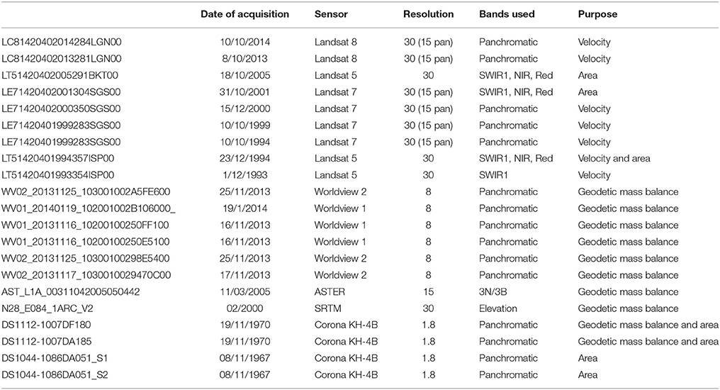
Table 1. The data used in this study and the purpose of each data source.

Corona Imagery

Corona is high-resolution (1.8 m) imagery acquired between 1960 and 1972 under the US Key Hole program, which was subsequently declassified in 1995 (Dashora et al., 2007). Corona imagery provides an invaluable dataset for glaciologists, but contains severe distortions that must be removed during the processing. Two Corona stereopairs were available that covered parts of the Manaslu region. The first stereopair from 1967 covered Ponkar Glacier and was partially affected by cloud. The Corona stereopair covering Ponkar Glacier were therefore only used for calculating the changes in glacier area and not geodetic glacier mass balance. The second Corona stereopair covered Thulagi, Punggeon and Hinang Glaciers and was from 1970. This image was cloud free and contained sufficient image contrast to generate a DEM.

As there is no mathematical model for Corona stereo-imagery, in order to generate a DEM the data must be processed in a non-metric approach which requires many tie-points in order to solve the interior and relative orientations (Schmidt et al., 2001; Galiatsatos et al., 2007). All the Corona imagery was processed in ERDAS Imagine 2015. We solved the relative orientation using many (mostly automatically generated) tie points, while the exterior orientation was solved using Ground Control Points (GCPs). The Ponkar Corona image was processed with 28 GCPs and 359 tie points while the Thulagi Corona image was processed with 75 GCPs and 1837 tie points. We used a combination of a 5 m RapidEye image from 2012 and the SRTM, as well as Google Earth imagery (after Surazakov and Aizen, 2010) as a source of GCP information, which although not ideal, allowed the products to be georeferenced enough for the DEMs to be later co-registered with the other DEMs (section DEM Co-registration). This allowed the images to be triangulated with an RMSE of <5 pixels. Orthomosaics from both datasets were exported at 2 m resolution, while the DEM from the Thulagi Corona image was exported at 8 m resolution using the eATE (enhanced Automatic Terrain Extraction) tool within ERDAS IMAGINE. All the DEMs were projected to UTM zone 45 N and geoid/ellipsoid differences were accounted for.

DEM Differencing

A combination of correlation masks and manual interpretation using the hillshade models was used to clean the DEMs and remove pixels with poor correlation scores (<0.6) or noticeable interpolation errors. This had the undesired effect of leaving large data voids over the accumulation areas of some of the glaciers. The DEMs were then resampled to the spatial resolution of the coarsest DEM (30 m). This was done using a median block statistics operation to avoid biases related to resolution variations of the DEMs and thus in their ability to depict terrain curvature and roughness (Paul, 2008; Gardelle et al., 2013).

DEM Co-registration

The method outlined by Nuth and Kääb (2011) was used to linearly co-register the DEMs by minimizing root mean square residuals of the elevation biases over stable terrain. Elevation biases are more noticeable on steeper slopes, therefore the elevation bias (dh) is normalized for slope (the tangent of the slope (tanα)) and plotted against the aspect (ψ):

$\begin{array}{ll}\frac{dh}{tan\alpha }=a.cos(b-\psi )+c& (1)\end{array}$

where a and b are the magnitude and direction of the co-registration shift, respectively, and c is the mean elevation bias between the DEMs divided by the mean surface slope. The co-registration process was iterated until the improvement of the standard deviation of the residual over stable terrain was less than 2%. The co-registration shifts are shown in Table 2. Figures 2A,B shows a graph of slope normalized elevation biases before and after planimetric co-registration.

FIGURE 2

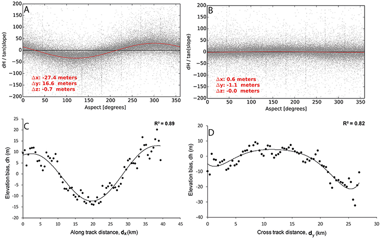
Figure 2. Plots of slope normalized terrain elevation differences between the 2013 SETSM DEM and the 2000 SRTM DEM over stable (non-glacier) terrain before co-registration (A) and after four iterations of co-registration (B). The co-registration shifts that were applied are shown in red text. (C) Shows the sixth-order polynomial fitted to the along-track elevation bias on the 1970 Corona DEM. (D) Shows the sixth-order polynomial fitted to the cross-track elevation bias on the 1970 Corona DEM.

TABLE 2

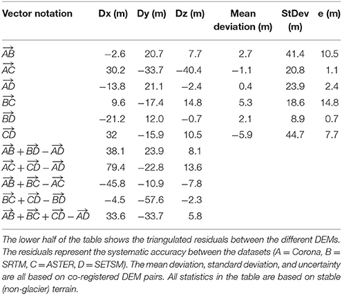
Table 2. The co-registration shifts between the different DEMs that was necessary before DEM differencing.

The complex nature of Corona data meant that a sixth-order polynomial was fitted to the elevation differences over stable terrain to account for both along- and across-track elevation biases (Figures 2C,D) (after Nuth and Kääb, 2011). The ASTER DEM contained elevation biases that were corrected with a second order polynomial.

Radar Penetration Correction

The SRTM dataset was acquired in C-and X-band, the former of which can penetrate into snow and ice by several meters (Rignot et al., 2001; Jaber et al., 2014). Various estimates have been made of the magnitude of this penetration in the Himalayas, ranging from 1.4–3.4 m (Gardelle et al., 2013) to 8–10 m (Kääb et al., 2012, 2015). While some studies have used uniform corrections to account for SRTM penetration, this does not take into account the varying depths of penetration with snow facies and altitude (Gardelle et al., 2012a; Kääb et al., 2012). Kääb et al. (2012) used ICESAT laser altimetry elevations to estimate SRTM penetration in various regions across the Himalayas. In this study we opted to use the corrections stated in Kääb et al. (2012) for clean ice (1.5 m) and firn/snow (2.3 m) in West Nepal. These techniques are however limited in the Himalayas where the accumulation and ablation seasons occur simultaneously, and frequent avalanches can distrust the snowline (Wu et al., 2014). We instead made the assumption that as the snow-line can be linked to the Equilibrium Line Altitude (ELA) (Rabatel et al., 2005), which in turn can be linked to the median elevation of glaciers in a steady state (Braithwaite and Raper, 2010), that snow-covered ice would be found predominantly above the median elevation, and bare ice would be found beneath it. These assumptions are however subject to further investigations. We applied the correction for firn/snow above the median elevation of each glacier and the correction for clean ice in debris-free areas below the median elevation.

Geodetic Glacier Mass Balance and Surface Elevation Change Analysis

The mean surface elevation change and geodetic mass balance were then determined. The geodetic mass balances were calculated using glacier outlines from the corresponding time periods. Pixels with (a) surface changes of more than 300 m or (b) elevation differences of greater than three standard deviations of the stable terrain elevation bias (after Gardelle et al., 2013) were masked out. Following Bolch et al. (2011) a spline interpolation was used to fill data gaps that were smaller than 10 pixels. Larger gaps were filled by fitting polynomials to mean elevation changes with altitude for each glacier (after Gardelle et al., 2013), although given the large SRTM data voids around Manaslu and Baudha, polynomial fitting was not possible for all glaciers. The conversion from volume-to-mass change was calculated by assuming a density of 850 kg m⁻³ following Huss (2013). Sorge's Law was assumed to hold true—that the relationship between density and depth in the firn pack does not vary with time (Bader, 1954).

Area Changes

Landsat images from 2013, 2005, and 2001 as well as Corona data from 1967/1970 (henceforth referred to as 1970) were used to assess the glacier area change (Table 1). The 2013 outlines were created by Robson et al. (2015) and were created semi-automatically using a combination of Landsat 8 imagery, a DEM and SAR Coherence data within an Object Based Image Analysis (OBIA) classification with additional manual corrections applied. The 2013 outlines were manually modified in order to create glacier outlines from 2005, 2001, and 1970. Noticeable breaks in slope morphology, visible vegetation change, exposed ice, or collapses in terminal moraines were used as indicators of underlying ice when mapping the debris-covered ice. The boundary between the clean ice and debris-covered ice was delineated for each set of outlines in order to monitor changes in the debris-covered area.

Glacier Velocity

Landsat images from 2013/2014, 1999/2000, and 1993/1994 (Table 1) were used for determining glacier velocities. The lack of image contrast on clean ice meant we restricted our velocity analysis to the debris-covered tongues of the glaciers, from the glacier terminus, to the transition between the clean ice and debris-covered ice. Prominent features on the debris-covered glaciers were tracked between sets of successive satellite images in order to determine the surface velocity. Features were matched using cross-correlation on orientation images (CCF-O) using the free software CIAS, developed by the University of Oslo (Kääb and Vollmer, 2000). Orientation images use the gradients between neighboring pixel values instead of the raw digital numbers, thereby reducing the influence of differences in scene illumination. Heid and Kääb (2012a) demonstrated that cross-correlating orientation images outperforms other image matching methods on debris-covered glaciers.

The image pairs were referenced together within CIAS using a Helmert Transformation with 15 to 20 points on stable terrain. Landsat 5 and 7 images were registered with RMSEs typically of 10–12 m, while Landsat 8 images were registered with RMSEs typically of less than 5 m.

Displacements were filtered by direction and magnitude. Displacements with a signal to noise ratio (SnR) lower than 0.5 were excluded. A 3 × 3 moving window was then used to remove displacement vectors that varied by more than 20% in magnitude or direction to the mean values. Some manual filtering was needed for removing matches associated with snow, shadow, or mass movements from the valley sides. Transverse profiles were plotted at the boundary between the clean ice and debris-covered ice in order to examine the changing debris-covered ice-flux. Additionally, glacier centrelines were generated automatically using the method of Kienholz et al. (2014) based on outlines from the Randolf Glacier Inventory (RGI) version 5.0 (Pfeffer et al., 2014) and the void-filled SRTM. The centrelines were manually edited to adapt them to changing glacier size in the older satellite imagery and the mean velocity extracted along the centrelines.

Hypsometric Analysis

The hypsometry of the 41 glaciers was computed for 2000 and 2013 using the SETSM and SRTM DEMs. The glacier outlines from 2013 and 1999 were divided into 100 m elevation bins and the area of each was determined in order to create hypsometric curves. A hypsometric index (HI) based on the maximum (H_max), median (H_med), and minimum (H_min), elevations of each glacier was calculated to characterize the glacier hypsometry based on the method of Jiskoot et al. (2009) and King et al. (2017):

$\begin{array}{ll}HI=\frac{H_{max}-H_{med}}{H_{med}-H_{min}}\text{ and if }0<\text{HI}<1\text{ then HI}=\frac{-1}{HI}& (2)\end{array}$

Glaciers were characterized by their HI as very top heavy (HI < −1.5), top heavy (−1.5 < HI < −1.2), equidimensional (−1.2 < HI < 1.2), bottom heavy (1.2 < HI < 1.5), or very bottom heavy (HI > 1.5).

Uncertainty Assessment

Glacier Outline Accuracy

Paul et al. (2013) estimate that the errors relating to the creation of glacier outlines are <5% when working with clean ice, but errors of up to 30% can arise due to debris-covered ice, stagnant ice, and shadows. In the absence of higher-resolution imagery or field data we cannot perform a rigorous error analysis of our glacier outlines.

Glacier Mass Balance Accuracy

The accuracy of the elevation changes was assessed by determining both the stochastic errors and the systematic errors (or biases) on terrain assumed to be stable (i.e., non-glacier rocky terrain). The systematic errors ($\overrightarrow{Z}$) between the DEMs was estimated by triangulating the DEM co-registration residuals (after Nuth et al., 2012). The z residual (Table 2) shows the vertical biases between the DEMs but is most likely an overestimate as these triangulations include only the linear residuals and not the polynomial adjustments made to the Corona and ASTER DEMs. The stochastic errors were quantified by comparing elevations over non-glacier terrain. We consider the 2013 SETSM DEM as a reference for the uncertainty analysis as it has the most spatial coverage and a high reported accuracy. Elevation differences were calculated for 2638 randomly chosen points over non-glacier terrain which had slopes of less than 30°. Extreme values (> ± 100 m) were not considered.

The standard error (SE) was calculated from the standard deviation over stable terrain (SD_STABLE) and the number of independent pixels included in the DEM differencing (n):

$\begin{array}{ll}SE=\frac{S{D}_{STABLE}}{\sqrt{n}}& (3)\end{array}$

where n considers the original number of pixels (N_tot), the pixel size (PS) and spatial autocorrelation (d):

$\begin{array}{ll}n=\frac{N_{tot}.PS}{2d}& (4)\end{array}$

We used a value of 400 m for the spatial correlation distance for the SETSM DEM and 600 m for all other DEMs based on the work of others (Bolch et al., 2011; King et al., 2017). DEM differencing uncertainty (e) was calculated by combining the standard error (SE) and the z-residual from the triangulation of the DEM co-registrations ($\overrightarrow{Z}$) using the sum of root mean squares (Equation 5). Additionally, ± 1.5 m uncertainty was added to equation 5 to account for the uncertainty related to SRTM penetration over clean ice and snow.

$\begin{array}{ll}e=\sqrt{S{E}^2+{\overrightarrow{Z}}^2}& (5)\end{array}$

Table 2 shows that the total DEM uncertainty errors (e) are <15 m for all DEM pairs. The Z triangulations and e values are largest for DEM pairs involving the ASTER DEM ($\overrightarrow{AC},\overrightarrow{BC},$ and $\overrightarrow{CD}$). The Corona DEM has a standard deviation of 23.9 m when compared with the SETSM DEM. Given the large time period between these datasets, and the image distortions associated with Corona data, these deviations are acceptable, although ~5 m higher than the standard deviations found by Bolch et al. (2011) and Pieczonka et al. (2013).

Glacier Velocity Accuracy

The uncertainty of the velocity measurements was determined by measuring displacements over terrain that was assumed to be stable. We restricted our error assessment to displacements on the terrain within 500 m of the terminus of Ponkar Glacier which had gentle slope, and free from shadow and snow cover in all images. The 2013/2014 displacements had the smallest mean displacement (2.0 m as opposed to 16.0 m for the 1999/2000 imagery and 5.5 m for the 1993/1994 imagery). In all cases the standard deviations are <9 m (8.2 m for 2013/2014, 3.2 m for 1999/2000, and 5.6 m for 1993/1994), smaller than the 15 m pixel size for the 2013/2014 and 1999/2000 imagery, and 30 m for the 1993/1994 images. The only results which are not significant (1 std) are for the glaciers that appear to be largely stagnant (for example Baudha Himal Glacier (G084684E28407N) and Northern Fukang Glacier (G084425E28837N).

Results

Our study area covers both the Himalayan Manaslu region to the south of the topographic divide (henceforth referred to as the southern glaciers) as well as a portion of the Tibetan Plateau to the north (henceforth referred to as the northern glaciers). Table 3 summarizes the changes in glacier area, geodetic mass balance, and surface elevation for the northern glaciers, southern glaciers, and the entire study region.

TABLE 3

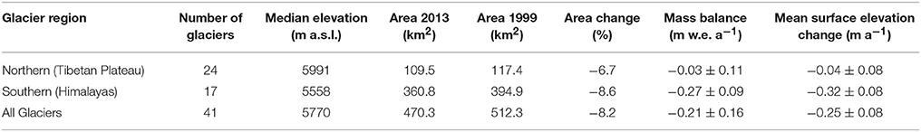
Table 3. Mean glacier changes for the glaciers on the Tibetan Plateau (Northern glaciers) and those south of the topographic divide in the Himalayas (Southern glaciers) between 1999/2000 and 2013.

Regional Changes between 2000 and 2013

The total glacier area of our study area in 2013 was 470.4 km² of which 84 km² (17.8%) was debris-covered ice. Between 2001 and 2013 the glacier area reduced by 42 km² (8.2%). Additionally, over half (52%) of the individual glaciers underwent an increase in debris-cover area over this time-period, with two glaciers (G084354E286669N and G084689E28511N) gaining over 1.5 km² of debris-cover, increases of 22 and 12% respectively.

The largest spatial coverage of elevation changes was obtained between 2000 and 2013 by comparing the SRTM and SETSM DEMs. The glaciers underwent a mean annual surface elevation change of −0.25 ± 0.08 m a⁻¹. Over the whole study area, the geodetic mass balance was found to be negative (−0.21 ± 0.16 m w.e. a⁻¹) with individual glacier mass balances varying from −0.79 ± 0.12 to + 0.30 ± 0.17 m w.e. a⁻¹. There are clear spatial patterns to the glacier change (Figure 3). Generally, the glaciers in the north (both those on the Tibetan Plateau, and those flowing south from Himlung) had less negative mass balances, while the glaciers located further to the south, especially those around Manaslu had more elevation differences.

FIGURE 3

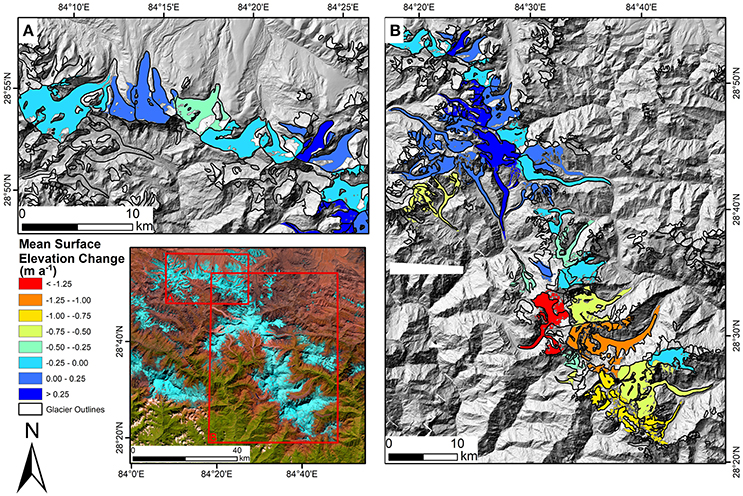
Figure 3. Mean annual surface elevation change per glacier between 2000 and 2013. Changes are shown for the northern glaciers (A) and southern glaciers (B). The background hillshade is based on the 2013 SETSM DEM.

Southern Glaciers

Glaciers south of the topographic divide are primarily debris-covered below 4600 m. Between 1999 and 2013 these glaciers lost 21.7 km² of ice (6.7% reduction in area). Many of the glacier termini remained in the same position, with the majority of glacier area changes occurring at the glacier margins and at the boundary between the clean ice and debris-covered ice. Some of the glaciers however underwent large terminus retreats. Thulagi glacier retreated 1.37 km between 1970 and 2013. Additionally, several large eastern flowing debris-covered glaciers (Punggeon Glacier: G084595E28536N and Hinang Glacier G084640E28489N : G084640E28489N) underwent large frontal retreats. Some debris-covered glaciers did not undergo sizable changes in area (for example G084539E28644N and G084550E28613N). Individual glacier area changes span from −9.0 to +1.1%.

Between 2000 and 2013, the southern glaciers in our study region had an average surface elevation change of −0.32 ± 0.08 m a⁻¹ which equates to a mean geodetic balance of −0.27 ± 0.09 m w.e. a⁻¹. There is a linear relationship (R² = 0.67) between elevation and the rates of glacier thinning over the entire glacier. The effects of the debris-cover appear to be complicated. Between ~4700 and 5700 m a.s.l rates of elevation change of debris-covered ice are greater than those of the clean ice components (Figure 4). The thinning rate generally increases as elevation decreases, reaching 1.56 ± 0.08 m a⁻¹ at ~4000 m a.s.l. Below 4000 m a.s.l. the thinning rate decreases to 0.78 ± 0.08 m a⁻¹ at ~3600 m a.s.l. before increasing to 1.10 ± 0.08 m a⁻¹ at 3300 m a.s.l.

FIGURE 4

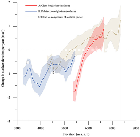
Figure 4. A comparison between elevation and the mean elevation change per 100 m elevation band between 2000 and 2013. Different responses to elevation are visible for the clean glaciers in the northern section of the study area (line A), the debris-covered components of the glaciers in the southern section of the study area (line B), and clean ice components of the southern glaciers (line C). Two noticeable deviations in the melt-rate (1, 2) are attributed to insulation of ice due to the build-up of supraglacial debris. The shaded areas represent one standard deviation of each elevation interval.

Northern Glaciers

The northern glaciers on the Tibetan Plateau are predominantly clean ice glaciers and have a higher mean elevation (5991 m a.s.l.) than the southern glaciers (5558 m a.s.l.) (Table 3). The glaciers lost an average of 6.7% of their area between 2000 and 2013. There appears to be an east-western trend in area change with G084132E28911NE and G084132E28911NW, in the far northwest of the study area, shrinking by 3.1 km² (13.5%) and 0.9 km² (16.5%). On the other hand G084424E28839N and G084461E28797N, two glaciers in the northeast of the study area and at approximately the same elevation, lost 0.2 km² (2.9%) and 0.3 km² (1.8%) of their area, respectively.

Despite losing 6.7% of their area, the northern glaciers were approximately in balance with a mean geodetic mass balance of −0.03 ± 0.11 m w.e. a⁻¹ and a mean surface elevation change of −0.04 ± 0.08 m a⁻¹ (Figures 3, 5). Individual geodetic mass balances ranged from −0.25 ± 0.15 to +0.30 ± 0.17 m w.e. a⁻¹. Some glaciers thickened over the majority of their surface, however these glaciers are situated at very high altitudes (minimum elevations > 6500 m a.s.l.). Thinning rates are inversely proportional to elevation with an R² of 0.87 (Figure 4). Ice situated at ~ 5400 m a.s.l. thinned by 1.66 ± 0.08 m a⁻¹ and ice at ~ 6700 m a.s.l. thickening by 0.99 ± 0.08 m a⁻¹.

FIGURE 5

Figure 5. Change in surface elevation for glaciers in the Manaslu region between 2000 and 2013. Changes are shown for the northern glaciers (A) and southern glaciers (B). The glacier outlines shown are from 2013. Background: Landsat 8 (26th December 2013).

Glacier Changes Over Different Time Periods

Our results show changing rates of both glacier area as well as glacier mass. Eight of the glaciers (~200 km²) were covered by Corona imagery from 1970. Between 1970 and 2013 these glaciers lost 37.9 km² of ice (17.9% area reduction), equating to a mean rate of −0.36 km² a⁻¹ between 1970 and 2001, −0.97 km² a⁻¹ between 2001 and 2005, and −2.28 km² a⁻¹ between 2005 and 2013. Over the entire study region, between 2001 and 2005 the total glacier area reduced at a rate of 6.4 km² a⁻¹ equating to 1.2% a⁻¹ while less glacier area per year was lost between 2005 and 2013 (2.06 km² a⁻¹ equating to 0.4% a⁻¹).

Twenty-one glaciers were covered by the 2013, 2005, and 2000 DEMs (Figure 1). The subset of these glaciers had a more negative mass balance (−0.44 ± 0.09 w.e. a⁻¹) than the regional average (−0.21 ± 0.16 w.e. a⁻¹). Considering that the subset excluded the more in-balance glaciers on the Tibetan Plateau this is not surprising. The highest regional glacier mass losses were found between 2000 and 2005 (−0.83 ± 0.74 m w.e. a⁻¹) although this varied through the region, with the three large glaciers flowing out of Manaslu losing most mass between 2005 and 2013 (−1.20 ± 0.87 m w.e. a⁻¹). The glaciers that were covered by the Corona data show changing rates of glacier loss. The rates of glacier downwasting have increased over the 43-year period, from −0.46 ± 0.03 m a⁻¹ between 1970 and 2000 to −0.99 ± 0.08 m a⁻¹ between 2000 and 2013. The geodetic mass balance for the three glaciers between 1970 and 2013 was −0.31 ± 0.12 m w.e. a⁻¹ (Figure 6) and −0.84 ± 0.11 m w.e. a⁻¹ between 2000 and 2013 (Table S2).

FIGURE 6

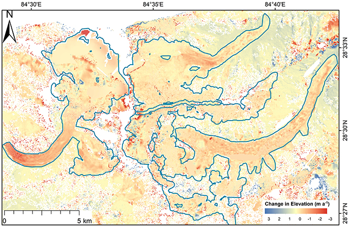
Figure 6. Mean annual change in surface elevation between 1970 and 2013 for Thulagi, Punggeon and Hinang Glaciers. The glacier outlines (shown in blue) are from 1970.

Glacier Hypsometry

In 2013 the southern glaciers had a mean HI of −1.29 (Table S1) indicating top heavy hypsometries with more area above the median glacier elevation. The northern glaciers on the other hand had a mean HI of 1.03 relating to a bottom heavy hypsometry. Figure 7 demonstrates the difference in hypsometries of northern and southern glaciers. Between 2000 and 2013 the southern glaciers have become more top heavy (HI change from −1.16 to −1.29) while the northern glaciers have become more bottom heavy (−1.14 to 1.03).

FIGURE 7

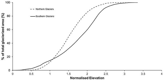
Figure 7. The hypsometry of the glaciers on the Tibetan Plateau (northern glaciers) is more top-heavy than that of the glaciers in the Himalayas (southern glaciers). Note that the elevation ranges have been normalized in order to compare northern and southern glaciers.

From the 2013 hypsometry, 70% of the total glacier area of the entire study region exists between 5200 and 6500 m a.s.l. This is also where the ELA approximated by the median elevation lies (~5748 m a.s.l.) meaning that a small rise in the ELA will expose a significant amount of ice to melting. Similar findings were also discussed by Shea et al. (2015) and King et al. (2017), who foresee a possibility of the debris-covered tongues becoming detached from the accumulation areas resulting in a bi-model hypsometry. In contrast, the bottom-heavy hypsometry of the northern glaciers implies that although a rise in ELA would expose ice to melting, future losses are likely to be limited by smaller areas of ice stored at higher elevations.

There is no statistical relationship between the glacier hypsometric index and glacier change, although some statements can be made. Punggeon Glacier (G084584E28535N) for example is very bottom heavy (HI = 1.81). The glacier has amongst the highest rates of surface elevation change in the region (−0.74 ± 0.08 m a⁻¹). Some of the glaciers storing large amounts of ice at higher elevations also have faster velocities, for example Ponkar Glacier: G084459E28695N; HI: −2.15 and Thulagi Glacier: G084549E28515N; HI: −1.25 velocities of 47.0 ± and 40.6 m a⁻¹ respectively.

Glacier Velocity

There is a large variation in glacier speed between individual glaciers (Figures 8, 9; Table S3), Ponkar Glacier (ID: G084456E28737N) and Thulagi Glacier (G084595E28536N) flowed at mean velocities in 2013/2014 of 47 ± 8.2 and 41 ± 8.2 m a⁻¹, respectively, while Baudha Himal Glacier (G084684E28407N) and Northern Fukang Glacier (G084425E28837N) have mostly stagnant debris-covered tongues with mean velocities of <3 m a⁻¹.

FIGURE 8

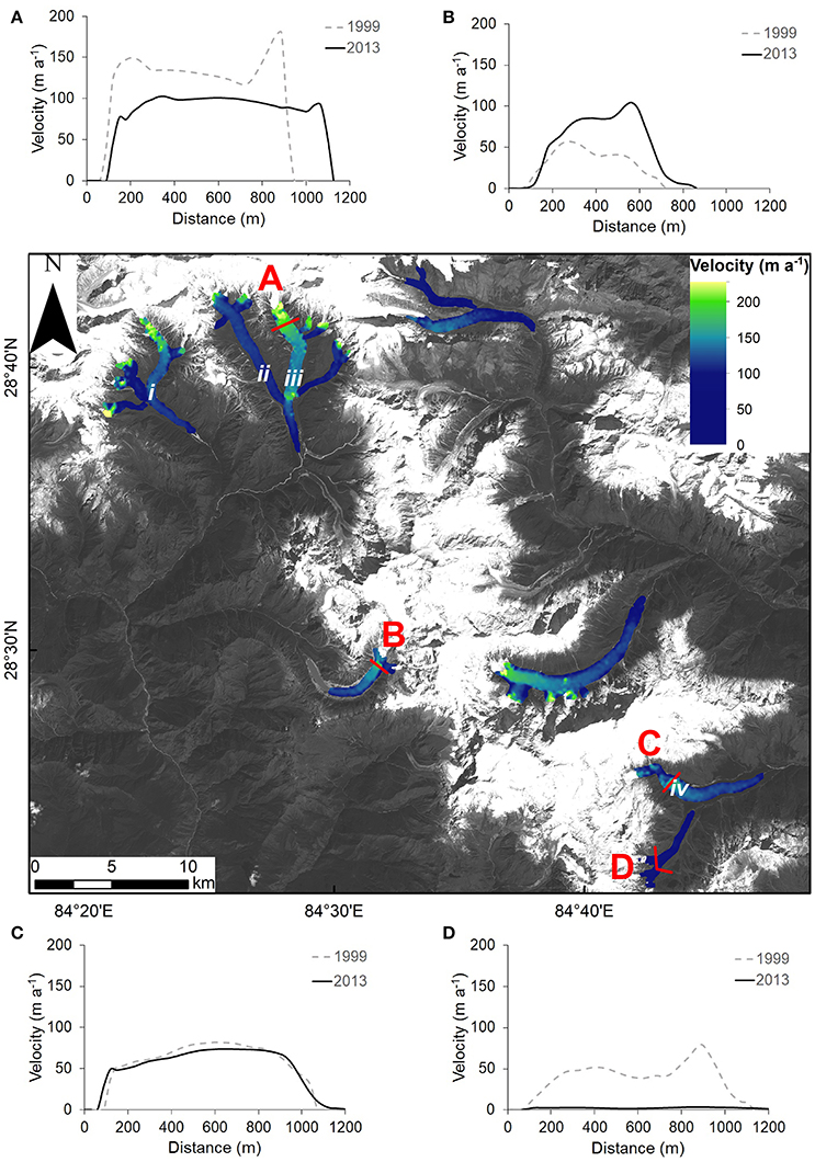
Figure 8. Annual surface velocities for the glaciers in the Manaslu Region for the year 2013/2014. (A–D) Show transverse velocity profiles at the boundary where the clean ice meets the debris-covered ice (transects shown as red lines) for (A) G084459E28695N (Ponkar glacier), (B) G084549E28515N (Thulagi glacier) (C) G084695E28384N (Himal Chuli glacier), and (D) G084759E28427N (Bhauda Himal glacier). Background: Landsat 8 (26th December 2013). The markings (i–iv) relate to the longitudinal profiles shown in Figure 9.

FIGURE 9

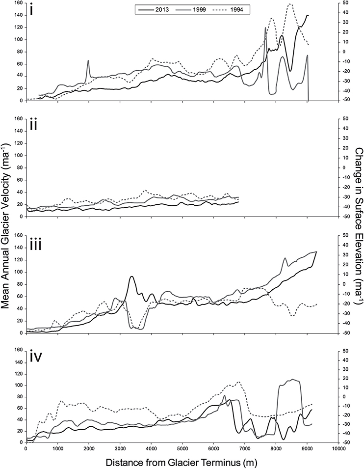
Figure 9. Velocity profiles from G084350E28675N (i), G084456E28737N W (ii), G084456E28737NE (iii), and G084684E28407N (iv) from 1993/1994, 1999/2000, and 2013/2013. The locations of these glaciers are shown in Figure 8.

There is no clear signal in glacier velocity changes in the region, with acceleration, deceleration, and constant velocities observed over the study period. Kechakyu Khola Glacier (G084425E28700N), Suti Glacier (G084354E28669NW), and Himal Chuli Glacier (G084759E28427N) have slowed by 12 m a⁻¹ (42.9%), 15.6 m a⁻¹ (29.0%), and 26.7 m a⁻¹ (45.7%) respectively between 1993/1994 and 2013/2014. Other glaciers have decelerated by a greater proportion, however these glaciers are flowing at such slow velocities (<3 m a⁻¹) that these changes in velocity are of a small magnitude. The termini of some glaciers such as Hinang Glacier (G084640E28489N) have noticeably stagnated (Figure 10). G084759E28427N has stagnated to the point of having near-zero velocities in 2013 (Figure 6D). Thulagi and Ponkar glaciers appear to show alternating patterns of glacier velocity, with slight accelerations in glacier velocity between 1993/1994 and 2013/2014 (5 and 6%, respectively). However, if the velocities are examined only between 1999/2000 and 2013/2014 then Ponkar Glacier decelerated by 10.4% while Thulagi Glacier accelerated by 27.3%. Regionally, the mean velocity varies only slightly between 1993/1994 and 1999/2000 (34.9 ± 5.6 and 32.4 ± 3.2 m a⁻¹ respectively) before decreasing by a mean of 5.2 m a⁻¹ (16.0%) between 1999/2000 and 2013/2014.

FIGURE 10

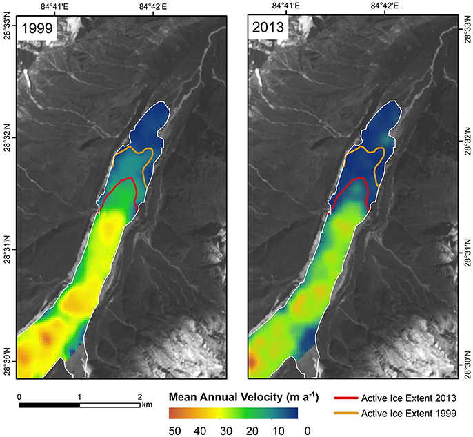
Figure 10. A comparison of ice velocities at Hinang Glacier (G084689E28511N) between 1999/2000 and 2013/2014. Despite no detectable changes in the extent of terminus (shown in a white dashed line), the terminus velocities have decreased. Background: Landsat 8 (26th December 2013).

Discussion

Spatial Variability of Glacier Change and Influencing Factors

There is a noticeable spatial variability of glacier mass change between the northern and southern glaciers, as well as within the northern and southern regions. We now explore some of the potential influencing factors of glacier mass balance within the Manaslu region.

Glacier Elevation and Hypsometry

The markedly distinct glacier responses between the northern and the southern glaciers seems to be broadly related to both glacier elevation and hypsometric class. The northern glaciers are situated at a higher median elevation (5991 as opposed to 5558 m a.s.l.) and have smaller altitudinal ranges (1887 m as opposed to 4529 m) than the southern glaciers. Many of the southern glaciers have altitudinal ranges in excess of 3000 m, with extensive lower-elevation debris-covered tongues that are losing mass.

The size of the accumulation area also appears to relate to some of the variation in the magnitude of changes between individual glaciers. For example, neighboring Ponkar (G084459E28695N) and Salpudanda (G084496E28676N) glaciers both flow in a southerly direction, yet have differing geodetic mass balances of +0.19 ± 0.08 and −0.02 ± 0.08 m w.e. a⁻¹ respectively. The difference could be explained by the much larger accumulation area feeding mass to Ponkar Glacier compared to Salpudanda Glacier. This large mass transfer can also be seen in the mean centreline surface velocities of Ponkar (47 ± 8.2 m a⁻¹) compared to Salpudanda (16 ± 8.2 m a⁻¹).

Importance of Supraglacial Debris

There is an inversely proportional relationship between glacier elevation and the rate of glacier thinning (Figure 4). This relationship varies for the northern (R² = 0.87) and southern glaciers (R² = 0.69) demonstrating the influence of supraglacial debris (Figure 4). The relationship between debris-covered ice thinning rates and elevation (Figure 4B) is more complex than the clean ice (Figures 4A,C). Although we do not possess sufficient data to examine the glacier thickness and composition, a number of statements can be made. A noticeable decrease in glacier elevation change rates at ~3500 m a.s.l. (Figure 4: 1) was also found by Benn et al. (2012) when glacier mass balance was modeled for Ngozumpa Glacier in the Everest Region. Although one must consider the range in termini elevations in the variations in elevation change rates, we interpret this peak as where the build-up of debris that is transported down-glacier becomes sufficient to offset glacier thinning. A similar deviation is visible at ~5300–5400 m a.s.l. (Figure 4: 2) which we attribute to a build-up of supraglacial debris where the clean ice entered the debris-covered ablation area. Between ~4700 and 5700 m a.s.l. the rates of glacier elevation range were higher for debris-covered ice than for the clean ice components of the southern glaciers. As these elevations are at the upper range of the debris-covered zone, the debris-thickness is likely less than at lower elevations. Critical thicknesses under which supraglacial debris amplified glacial melt range between 30 and 115 mm for High Mountain Asia (Reznichenko et al., 2010). Although we do not have debris-thickness field data, we speculate that the supraglacial thickness in these areas is sufficiently thin to increase the thinning rates relative to the clean ice. Additional variations in the glacier surface elevation change rates could potentially be explained by the changing distribution of supraglacial debris and the presence of supraglacial lakes and ice cliffs. Despite being responsible for up to 20% of glacier ablation (Nuimura et al., 2012; Immerzeel et al., 2014; Kraaijenbrink et al., 2016), many of these features are too small to detect on satellite imagery, with Watson et al. (2016) reporting that 30-m Landsat imagery is incapable of capturing 77–99% of the total number of supraglacial ponds on glaciers in the Everest region.

In addition to the presence of supraglacial debris, the characteristics of it are also an important influence on the mass changes of the glaciers. We do not have data about the debris-thickness, yet certain inferences can be made from remote sensing data. Himal Chuli Glacier (G084759E28427N) for example passes through a narrow valley. A large rockfall (~0.80 km²) hit the upper ablation area of the glacier in 2002, as is visible on satellite imagery (Figure 11). The effects of the rockfall material thickening the debris cover can be clearly seen with an area of reduced elevation loss between 2000 and 2013. A supraglacial lake formed on the rockfall deposit in 2011 and drained about 6 months later. The influence of this lake on the glacier ablation can be seen in Figure 11F; where the area formerly filled by the lake shows higher thinning rates than the surrounding glacier terrain. We speculate that there are numerous small scale supraglacial ponds and ice-cliffs across the Manaslu region that although important for governing glacier mass balance, are undetectable without finer-scale imagery.

FIGURE 11

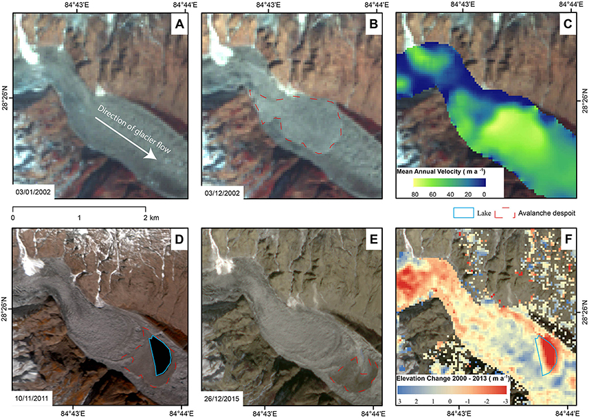
Figure 11. A large rockfall hit Himal Chuli Glacier in 2002 (visible on B). The rockfall deposit has since been transported downglacier. The surface velocity increases as the glacier flows out of the bend (C). The glacier is flowing toward the south-east. A large lake formed in 2011 (D) which drained the following year €. Nevertheless, the location of the lake correlates with an area of increased elevation loss (F). The satellite imagery in (D) is RapidEye imagery, (E) is Sentinel 2, the remaining satellite images are Landsat imagery.

Spatial Variation in Glacier Velocity

As outlined above, the spatial variability of glacier surface velocities between individual glaciers appears to broadly relate to the altitudinal range and hypsometric class of the glaciers. There is also considerable variation in velocity within individual glaciers.

An interesting example of complex glacier change is Himal Chuli Glacier (Figure 11). Himal Chuli Glacier exhibits a noticeable increase in surface velocity as the glacier flows out of the bend, with higher velocities especially apparent toward the center of the glacier. The increase in glacier velocity and associated glacier elevation change decrease are likely due to vertical emergence caused by compression and a steeper gradient in the bend in the valley (Hooke, 2005). A similar effect has been observed on Lirung Glacier in the Langtang valley (Immerzeel et al., 2014).

Variation in Debris-Cover Ice-Flux

As discussed above, supraglacial debris is an important factor in controlling the magnitude of glacier thinning and mass loss. Glacier velocity is an important parameter, responsible for transporting mass from the accumulation areas to the ablation areas and therefore maintaining the flux of supraglacial debris into the ablation area. The glacier velocity varies throughout the region from stagnant (~0 m a⁻¹) to very active flow (>40 m a⁻¹). Figure 8 shows transverse velocity profiles at the boundary between the clean ice and the debris-covered. In three out of four cases, the amount of ice being transported into the debris-covered ice has decreased. Ongoing glacier stagnation and a reduction in velocity will allow more supraglacial debris to accumulate from slope processes and debris-flows (Anderson and Mackintosh, 2012), while debris thickness also increases with glacier thinning due to englacial debris melting out. Additionally, over half of the debris-covered glaciers underwent an increase in debris-covered area, which can be associated with negative glacier mass balances (Kirkbride and Deline, 2013; Herreid et al., 2017). The combination of both these processes will exacerbate glacial stagnation and further weaken the relationship between climate and changes in glacier area and mass balance. On the other hand, when the glacier velocity increases, as is the case with Thulagi glacier, the rate of debris-thickness change is expected to decrease, while additionally, an increased velocity can augment the fracturing and lead to more exposed ice on the debris-covered surface, leading to increased mass losses.

Thulagi Glacier and GLOF Risk

Dona Lake expanded from 0.50 km² in 1970 to 0.93 km² in 2013. During this time the glacier downwasted at a mean rate of 0.49 ± 0.03 m a⁻¹, the highest rates in the Manaslu region. Between 1970 and 2001 Thulagi Glacier terminated in Dona Lake, however by 2005 the glacier appears to have retreated onto land. While moraine subsidence between 1996 and 2009 occurred at a rate of ~1 m a⁻¹, lake surface elevations lowered by 0.3 to −0.5 m a⁻¹ between 1996 and 2009 (Mool, 2011). This implies that the lake discharge through the old moraine is greater than the water added to the lake from the melting of the glacier. With the glacier now terminating on land it seems unlikely that lake will continue to expand, even with increasing glacier melt rates.

In addition to losing mass, Thulagi glacier exhibits complex patterns in velocity. The glacier velocity decelerated between 1993 and 1999 by 16.7%, followed by an acceleration in velocity of 29.7% between 1999 and 2013. A similar trend is seen in the glacier hypsometry. Between 1970 (HI = −1.18) and 2000 (HI = −1.37) Thulagi glacier become more top heavy, while between 2000 and 2013 Thulagi glacier become less top heavy (HI = −1.25).

Analytical Uncertainties

We calculated the DEM differencing uncertainties in terms of stochastic error and systematic error. The stochastic error was based on the standard error and the mean elevation difference on stable terrain. Magnusson et al. (2016) showed how standard methods for quantifying DEM differencing uncertainties neglect the spatial dependence of DEM errors, and as such typically overestimate uncertainties. It should therefore be noted that our uncertainty analysis is conservative.

Even with our conservative error estimation, 64% of our surface elevation change results are significantly different from zero, as well as eight of the 10 regional averages. Fifty-eight percent of our geodetic mass balance results however were significant, with only the regional average from 1970 to 2013 being larger than the associated error bars. As stated by Gardelle et al. (2013), the largest component of the uncertainty is the estimation of the SRTM penetration. Values range from 1 to 10 m (Gardelle et al., 2013; Kääb et al., 2015; Berthier et al., 2016) which is considerably greater than the stochastic error. Additionally sources of error include the assumed constant density of 850 kg m⁻³ across the entire glacier (Huss, 2013).

In the absence of a more rigorous method, we estimated uncertainties for our velocity results based on ± one standard deviation. This assumes that no displacements have occurred on non-glacier terrain. Rockfalls and movements are common in the High Himalayas meaning our uncertainty estimates are most likely overestimated. Nevertheless, 94% of our velocity measurements are significant, in addition to all three regional averages.

Comparison with Other Work

Our findings add to the consensus of strong yet spatially variable glacier mass losses across the Himalayas. In recent years, studies looking at geodetic mass balances of Himalayan glaciers have become more common (Gardelle et al., 2013; Pellicciotti et al., 2015; Bhattacharya et al., 2016; Ragettli et al., 2016; Brun et al., 2017). Due to the differing climatic regimes across the Himalayas, we restrict our comparisons to the Central Himalayas and the Everest Region. Our results are comparable to surface elevation change rates in the Everest Region of −0.32 ± 0.08 m a⁻¹ between 1970 and 2007 (Bolch et al., 2011) and −0.28 ± 0.42 m a⁻¹ between 1974 and 2006 in the Langtang Himal (Ragettli et al., 2016). This is very comparable to our result of −0.36 ± 0.03 m a⁻¹ between 1970 and 2013. Both our results and the findings of Bolch et al. (2012) indicate increases in the rate of mass loss between 2000 and 2013 relative to other time periods.

When looking at shorter time periods, Kääb et al. (2012) found a mean annual surface elevation change of −0.21 ± 0.05 m a⁻¹ over the entire Hindu Kush Himalaya Region between 2003 and 2008, with some regions losing as much as −0.66 m a⁻¹. Brun et al. (2017) found mean annual geodetic mass balances between 2000 and 2016 of −0.33 ± 0.20 and −0.34 ± 0.09 m w.e. a⁻¹ for East and West Nepal, respectively. The losses we found between 2000 and 2013 of −0.25 ± 0.08 m a⁻¹ therefore compares well with these regional averages. Our results of geodetic mass balance for the southern glaciers between 2000 and 2013 (−0.27 ± 0.09 m w.e. a⁻¹) are less negative than the results found by Gardelle et al. (2013) for western Nepal (−0.32 ± 0.13 m w.e.a⁻¹) but is in line with the result from the Everest region (−0.26 ± 0.13 m w.e.a⁻¹) over roughly the same time period. Bolch et al. (2011) found a more negative mass balance of −0.79 ± 0.52 m w.e.a⁻¹ between 2002 and 2009 in the Everest Region. Our geodetic mass balance between 2005 and 2013 (−0.74 ± 0.55 m w.e.a⁻¹) is more comparable to their findings.

Our estimate of the ELA based on the median glacier elevation of 5748 m is in broad agreement with the estimate of ~5600 m for the ELA in the central Himalayas reported by (Bolch et al., 2012) and for Western Nepal of 5590 ± 138 m by Gardelle et al. (2013).

Quincey et al. (2009) found that the debris-covered glaciers in the Everest region flowed at ~20 m a⁻¹, which is slower than our mean result of 27 ± 8.2 m a⁻¹ in 2013. Kääb (2005) found that the debris-covered glaciers in Bhutan were flowing at higher rates of between 20 and 50 m a⁻¹. There is less work concerning changes in glacier velocity over time, and the work that does exist often find contradictory results of how glacier velocity has varied. Heid and Kääb (2012b) observed reductions in glacier velocity in areas with negative mass balances, including a 43% reduction in velocity in their nearest study site to the Manaslu region, the Pamir Mountains between 2001 and 2010. Haritashya et al. (2015) found reductions in glacier velocity of Khumbu glacier between 2003 and 2008 of between 10 and 20% while Bhattacharya et al. (2016) found a 6.7% decrease from 1996 to 2013 in the Indian Himalaya. The reduction we measured in this study of 15.0% between 1999 and 2013 is in line with these values.

Conclusion

This study presents varied and complex glacier changes in the Manaslu region of Nepal. Twelve percent of glaciers had an area change of <1% between 2001 and 2013 while 52% of glaciers had an increase in the area of debris-cover over this time period. Changes in glacier area, geodetic mass balance and velocity change are all negative at a regional scale yet glaciers with large accumulation areas or high elevations are approximately in balance. Rates of change are becoming more negative over the last decade compared to longer timescales. The effect of debris-covered ice is seen in different areas to both exacerbate and dampen rates of glacier elevation change. We have seen some evidence from our study area of the importance of supraglacial lakes, although with higher resolution satellite imagery we speculate that many smaller supraglacial ponds and ice cliffs could be observed and correlated with surface elevation changes. The ice-flux entering the debris-zone has reduced between 1999/2000 and 2013/2014. We suggest that glacier stagnation and debris melt-out allow supraglacial debris to accumulate, thereby further insulating the underlying ice and dampening the glacier area or elevation change. Given the suitability of Landsat 8 and Sentinel 2 data for large-scale velocity mapping (Fahnestock et al., 2015; Kääb et al., 2016), future work should investigate seasonal changes to glacier velocity. Research is also needed to study how debris-composition and the presence of supraglacial ponds and exposed ice influences glacier mass balance over short- and long-term time scales.

Author Contributions

BR, SD, and CN devised the study. BR, CN, LG, and MH processed the data. BR and PN generated the figures. All authors contributed to writing and editing the manuscript.

Funding

Funding was provided from the Department of Geography, University of Bergen, as well as the Meltzer foundation and RESCLIM.

Conflict of Interest Statement

The authors declare that the research was conducted in the absence of any commercial or financial relationships that could be construed as a potential conflict of interest.

Acknowledgments

We would like to thank the three reviewers for their thorough and comprehensive feedback which improved the quality of the manuscript. The authors would like to thank Asha Badadur Rai (www.adventurousnepal.com) and his family for organizing all the logistics and practicalities of our fieldwork trekking around the Manaslu Conservation Area in both 2013 and 2014 and making us very welcome in Nepal. Thanks to Christian Kienholz who generated the centrelines for the glaciers. The authors are grateful to Owen King, Duncan Quincey, and Max Koller who read through this manuscript. Thanks also to the colleagues at the Department of Geography, University of Bergen and the Department of Geoscience, University of Oslo for their useful feedback and support during the writing process of this paper. We are grateful to ResClim and Melzer for funding that supported this work. CN acknowledges funding from the European Union/ERC (grant no. 320816) and ESA (project Glaciers_CCI, 4000109873/14/I-NB). Thanks to NASA and the USGS for the provision of Landsat, ASTER, Corona and SRTM Data and to Ian Howat for the SETSM data.

Supplementary Material

The Supplementary Material for this article can be found online at: https://www.frontiersin.org/articles/10.3389/feart.2018.00012/full#supplementary-material

References

Ageta, Y., and Higuchi, K. (1984). Estimation of mass balance components of a summer-accumulation type glacier in the Nepal Himalaya. Geogr. Ann. Ser. A. Phys. Geogr. 66, 249–255. doi: 10.1080/04353676.1984.11880113

CrossRef Full Text | Google Scholar

Anderson, B., and Mackintosh, A. (2012). Controls on mass balance sensitivity of maritime glaciers in the Southern Alps, New Zealand: the role of debris cover. J. Geophys. Res. 117:F01003. doi: 10.1029/2011JF002064

CrossRef Full Text | Google Scholar

Bader, H. (1954). Sorge's Law of densification of snow on high polar glaciers. J. Glaciol. 2, 319–323. doi: 10.1017/S0022143000025144

CrossRef Full Text | Google Scholar

Bajracharya, S. R. (2014). Glacier Status in Nepal and Decadal Change from 1980 to 2010 Based on Landsat Data. Kathmandu: International Centre for Integrated Mountain Development.

Bajracharya, S. R., Maharjan, S. B., and Shrestha, F. (2014). The status and decadal change of glaciers in Bhutan from the 1980s to 2010 based on satellite data. Ann. Glaciol. 55, 159–166. doi: 10.3189/2014AoG66A125

CrossRef Full Text | Google Scholar

Benn, D. I., Bolch, T., Hands, K., Gulley, J., Luckman, A., Nicholson, L. I., et al. (2012). Response of debris-covered glaciers in the Mount Everest region to recent warming, and implications for outburst flood hazards. Earth Sci. Rev. 114, 156–174. doi: 10.1016/j.earscirev.2012.03.008

CrossRef Full Text | Google Scholar

Benn, D. I., and Owen, L. A. (1998). The role of the Indian summer monsoon and the mid-latitude westerlies in Himalayan glaciation: review and speculative discussion. J. Geolog. Soc. 155, 353–363. doi: 10.1144/gsjgs.155.2.0353

CrossRef Full Text | Google Scholar

Benn, D. I., and Lehmkuhl, F. (2000). Mass balance and equilibrium-line altitudes of glaciers in high-mountain environments. Quat. Int. 65–66, 15–29. doi: 10.1016/S1040-6182(99)00034-8

CrossRef Full Text

Berthier, E., Cabot, V., Vincent, C., and Six, D. (2016). Decadal region-wide and glacier-wide mass balances derived from multi-temporal ASTER satellite digital elevation models. Validation over the Mont-Blanc area. Front. Earth Sci. 4:63. doi: 10.3389/feart.2016.00063

CrossRef Full Text | Google Scholar

Bhattacharya, A., Bolch, T., Mukherjee, K., Pieczonka, T., Kropáček, J., and Buchroithner, M. F. (2016). Overall recession and mass budget of Gangotri Glacier, Garhwal Himalayas, from 1965 to 2015 using remote sensing data. J. Glaciol. 62, 1115–1133. doi: 10.1017/jog.2016.96

CrossRef Full Text | Google Scholar

Bolch, T., Buchroithner, M. F., Peters, J., Baessler, M., and Bajracharya, S. (2008). Identification of glacier motion and potentially dangerous glacial lakes in the Mt. Everest region/Nepal using spaceborne imagery. Nat. Haz. Earth Syst. Sci. 8, 1329–1340. doi: 10.5194/nhess-8-1329-2008

CrossRef Full Text | Google Scholar

Bolch, T., Kulkarni, A., Kääb, A., Huggel, C., Paul, F., Cogley, J. G., et al. (2012). The state and fate of Himalayan glaciers. Science 336, 310–314. doi: 10.1126/science.1215828

PubMed Abstract | CrossRef Full Text | Google Scholar

Bolch, T., Pieczonka, T., and Benn, D. (2011). Multi-decadal mass loss of glaciers in the Everest area (Nepal Himalaya) derived from stereo imagery. Cryosphere 5, 349–358. doi: 10.5194/tc-5-349-2011

CrossRef Full Text | Google Scholar

Braithwaite, R., and Raper, S. (2010). Estimating equilibrium-line altitude (ELA) from glacier inventory data. Ann. Glaciol. 50, 127–132. doi: 10.3189/172756410790595930

CrossRef Full Text | Google Scholar

Brun, F., Berthier, E., Wagnon, P., Kääb, A., and Treichler, D. (2017). A spatially resolved estimate of High Mountain Asia glacier mass balances from 2000 to 2016. Nat. Geosci. 10, 668–673. doi: 10.1038/ngeo2999

PubMed Abstract | CrossRef Full Text | Google Scholar

Brun, F., Buri, P., Miles, E. S., Wagnon, P., Steiner, J., Berthier, E., et al. (2016). Quantifying volume loss from ice cliffs on debris-covered glaciers using high-resolution terrestrial and aerial photogrammetry. J. Glaciol. 62, 684–695. doi: 10.1017/jog.2016.54

CrossRef Full Text | Google Scholar

Carrivick, J. L., and Tweed, F. S. (2016). A global assessment of the societal impacts of glacier outburst floods. Glob. Planet. Change 144, 1–16. doi: 10.1016/j.gloplacha.2016.07.001

CrossRef Full Text | Google Scholar

Copland, L., Pope, S., Bishop, M. P., Shroder, J. F., Clendon, P., Bush, A., et al. (2009). Glacier velocities across the central Karakoram. Ann. Glaciol. 50, 41–49. doi: 10.3189/172756409789624229

CrossRef Full Text | Google Scholar

Dashora, A., Lohani, B., and Malik, J. N. (2007). A repository of earth resource information–CORONA satellite programme. Curr. Sci. 92, 926–932.

Google Scholar

De Ferranti, J. (2012). Viewfinder Panorama DEMs [Online]. Available online at: http://www.viewfinderpanoramas.org/

Dehecq, A., Gourmelen, N., and Trouve, E. (2015). Deriving large-scale glacier velocities from a complete satellite archive: application to the Pamir–Karakoram–Himalaya. Remote Sens. Environ. 162, 55–66. doi: 10.1016/j.rse.2015.01.031

CrossRef Full Text | Google Scholar

Department of Hydrology and Meteorology (Government Of Nepal). (2014). Interpolated 12 km Temperature and Rainfall Mean Annual Data (1970–2010) [Online]. Kathmandu. Available online at: http://dhm.gov.np/

Fahnestock, M., Scambos, T., Moon, T., Gardner, A., Haran, T., and Klinger, M. (2015). Rapid large-area mapping of ice flow using Landsat 8. Remote Sens. Environ. 185, 84–94. doi: 10.1016/j.rse.2015.11.023

CrossRef Full Text | Google Scholar

Galiatsatos, N., Donoghue, D. N., and Philip, G. (2007). High resolution elevation data derived from stereoscopic CORONA imagery with minimal ground control. Photogrammetr. Eng. Remote Sens. 73, 1093–1106. doi: 10.14358/PERS.73.9.1093

CrossRef Full Text | Google Scholar

Gardelle, J., Berthier, E., and Arnaud, Y. (2012a). Impact of resolution and radar penetration on glacier elevation changes computed from DEM differencing. J. Glaciol. 58, 419–422. doi: 10.3189/2012JoG11J175

CrossRef Full Text | Google Scholar

Gardelle, J., Berthier, E., and Arnaud, Y. (2012b). Slight mass gain of Karakoram glaciers in the early twenty-first century. Nat. Geosci. 5, 322–325. doi: 10.1038/ngeo1450

CrossRef Full Text | Google Scholar

Gardelle, J., Berthier, E., Arnaud, Y., and Kaab, A. (2013). Region-wide glacier mass balances over the Pamir-Karakoram-Himalaya during 1999-2011 (vol 7, pg 1263, 2013). Cryosphere 7, 1885–1886. doi: 10.5194/tc-7-1885-2013

CrossRef Full Text | Google Scholar

Girod, L., Nuth, C., Kääb, A., Mcnabb, R., and Galland, O. (2017). MMASTER: improved ASTER DEMs for elevation change monitoring. Remote Sens. 9:704. doi: 10.3390/rs9070704

CrossRef Full Text | Google Scholar

Haritashya, U. K., Pleasants, M. S., and Copland, L. (2015). Assessment of the evolution in velocity of two debris-covered valley glaciers in Nepal and New Zealand. Geogr. Ann. 97, 737–751. doi: 10.1111/geoa.12112

CrossRef Full Text | Google Scholar

Heid, T., and Kääb, A. (2012a). Evaluation of existing image matching methods for deriving glacier surface displacements globally from optical satellite imagery. Remote Sens. Environ. 118, 339–355. doi: 10.1016/j.rse.2011.11.024

CrossRef Full Text | Google Scholar

Heid, T., and Kääb, A. (2012b). Repeat optical satellite images reveal widespread and long term decrease in land-terminating glacier speeds. Cryosphere 6, 467–478. doi: 10.5194/tc-6-467-2012

CrossRef Full Text | Google Scholar

Herreid, S., Pellicciotti, F., Ayala, A., Chesnokova, A., Kienholz, C., Shea, J., et al. (2017). Satellite observations show no net change in the percentage of supraglacial debris-covered area in northern Pakistan from 1977 to 2014. J. Glaciol. 61, 524–536. doi: 10.3189/2015JoG14J227

CrossRef Full Text | Google Scholar

Hooke, R. L. (2005). Principles of Glacier Mechanics. Cambridge, UK: Cambridge University Press.

Google Scholar

Huss, M. (2013). Density assumptions for converting geodetic glacier volume change to mass change. Cryosphere 7, 877–887. doi: 10.5194/tc-7-877-2013

CrossRef Full Text | Google Scholar

Immerzeel, W., Kraaijenbrink, P., Shea, J., Shrestha, A., Pellicciotti, F., Bierkens, M., et al. (2014). High-resolution monitoring of Himalayan glacier dynamics using unmanned aerial vehicles. Remote Sens. Environ. 150, 93–103. doi: 10.1016/j.rse.2014.04.025

CrossRef Full Text | Google Scholar

Immerzeel, W. W., Van Beek, L. P., and Bierkens, M. F. (2010). Climate change will affect the Asian water towers. Science 328, 1382–1385. doi: 10.1126/science.1183188

PubMed Abstract | CrossRef Full Text | Google Scholar

Jaber, W. A., Floricioiu, D., and Rott, H. (2014). “Glacier dynamics of the Northern Patagonia Icefield derived from SRTM, TanDEM-X and TerraSAR-X data,” in Geoscience and Remote Sensing Symposium (IGARSS), 2014 IEEE International (Québec City, QC), 4018–4021.

Google Scholar

Jiskoot, H., Curran, C. J., Tessler, D. L., and Shenton, L. R. (2009). Changes in Clemenceau icefield and Chaba Group glaciers, Canada, related to hypsometry, tributary detachment, length–slope and area–aspect relations. Ann. Glaciol. 50, 133–143. doi: 10.3189/172756410790595796

CrossRef Full Text | Google Scholar

Juen, M., Mayer, C., Lambrecht, A., Han, H., and Liu, S. (2014). Impact of varying debris cover thickness on ablation: a case study for Koxkar Glacier in the Tien Shan. Cryosphere 8:77. doi: 10.5194/tc-8-377-2014

CrossRef Full Text | Google Scholar

Kääb, A. (2005). Combination of SRTM3 and repeat ASTER data for deriving alpine glacier flow velocities in the Bhutan Himalaya. Remote Sens. Environ. 94, 463–474. doi: 10.1016/j.rse.2004.11.003

CrossRef Full Text | Google Scholar

Kääb, A., Berthier, E., Nuth, C., Gardelle, J., and Arnaud, Y. (2012). Contrasting patterns of early twenty-first-century glacier mass change in the Himalayas. Nature 488, 495–498. doi: 10.1038/nature11324

PubMed Abstract | CrossRef Full Text | Google Scholar

Kääb, A., Treichler, D., Nuth, C., and Berthier, E. (2015). Brief Communication: contending estimates of 2003–2008 glacier mass balance over the Pamir–Karakoram–Himalaya. Cryosphere 9, 557–564. doi: 10.5194/tc-9-557-2015

CrossRef Full Text | Google Scholar

Kääb, A., and Vollmer, M. (2000). Surface geometry, thickness changes and flow fields on creeping mountain permafrost: automatic extraction by digital image analysis. Permafr. Periglac. Process. 11, 315–326. doi: 10.1002/1099-1530(200012)11:4<315::AID-PPP365>3.0.CO;2-J

CrossRef Full Text | Google Scholar

Kääb, A., Winsvold, H. S., Altena, B., Nuth, C., Nagler, T., and Wuite, J. (2016). Glacier remote sensing using sentinel-2. part I: radiometric and geometric performance, and application to ice velocity. Remote Sens. 8:598. doi: 10.3390/rs8070598

CrossRef Full Text | Google Scholar

Kienholz, C., Rich, J., Arendt, A., and Hock, R. (2014). A new method for deriving glacier centerlines applied to glaciers in Alaska and northwest Canada. Cryosphere 8, 503–519. doi: 10.5194/tc-8-503-2014

CrossRef Full Text | Google Scholar

King, O., Quincey, D. J., Carrivick, J. L., and Rowan, A. V. (2017). Spatial variability in mass loss of glaciers in the Everest region, central Himalayas, between 2000 and 2015. Cryosphere 11, 407–426. doi: 10.5194/tc-11-407-2017

CrossRef Full Text | Google Scholar

Kirkbride, M. P., and Deline, P. (2013). The formation of supraglacial debris covers by primary dispersal from transverse englacial debris bands. Earth Surf. Process. Landf. 38, 1779–1792 doi: 10.1002/esp.3416

CrossRef Full Text | Google Scholar

Kraaijenbrink, P. D. A., Shea, J. M., Pellicciotti, F., Jong, S. M. D., and Immerzeel, W. W. (2016). Object-based analysis of unmanned aerial vehicle imagery to map and characterise surface features on a debris-covered glacier. Remote Sens. Environ. 186, 581–595. doi: 10.1016/j.rse.2016.09.013

CrossRef Full Text | Google Scholar

Magnusson, E., Belart, J. M. C., Palsson, F., Agustsson, H., and Crochet, P. (2016). Geodetic mass balance record with rigorous uncertainty estimates deduced from aerial photographs and lidar data-Case study from Drangajokull ice cap, NW Iceland. Cryosphere 10, 159–177. doi: 10.5194/tc-10-159-2016

CrossRef Full Text | Google Scholar

Maurer, J., and Rupper, S. (2015). Tapping into the Hexagon spy imagery database: a new automated pipeline for geomorphic change detection. ISPRS J. Photogr. Remote Sens. 108, 113–127. doi: 10.1016/j.isprsjprs.2015.06.008

CrossRef Full Text | Google Scholar

Maussion, F., Scherer, D., Mölg, T., Collier, E., Curio, J., and Finkelnburg, R. (2014). precipitation seasonality and variability over the Tibetan Plateau as resolved by the High Asia Reanalysis. J. Clim. 27, 1910–1927. doi: 10.1175/JCLI-D-13-00282.1

CrossRef Full Text | Google Scholar

Mool, P. K. (2011). Glacial Lakes and Glacial Lake Outburst Floods in Nepal. Kathmandu: International Centre for Integrated Mountain Development.

Nagai, H., Fujita, K., Nuimura, T., and Sakai, A. (2013). Southwest-facing slopes control the formation of debris-covered glaciers in the Bhutan Himalaya. Cryosphere 7, 1303–1314. doi: 10.5194/tc-7-1303-2013

CrossRef Full Text | Google Scholar

Neckel, N., Loibl, D., and Rankl, M. (2017). Recent slowdown and thinning of debris-covered glaciers in south-eastern Tibet. Earth Planet. Sci. Lett. 464, 95–102. doi: 10.1016/j.epsl.2017.02.008

CrossRef Full Text | Google Scholar

Noh, M.-J., and Howat, I. M. (2015). Automated stereo-photogrammetric DEM generation at high latitudes: surface extraction with TIN-based search-space minimization (SETSM) validation and demonstration over glaciated regions. GISci. Remote Sens. 52, 198–217. doi: 10.1080/15481603.2015.1008621

CrossRef Full Text | Google Scholar

Nuimura, T., Fujita, K., Yamaguchi, S., and Sharma, R. R. (2012). Elevation changes of glaciers revealed by multitemporal digital elevation models calibrated by GPS survey in the Khumbu region, Nepal Himalaya, 1992–2008. J. Glaciol. 58, 648–656. doi: 10.3189/2012JoG11J061

CrossRef Full Text | Google Scholar

Nuimura, T., Sakai, A., Taniguchi, K., Nagai, H., Lamsal, D., Tsutaki, S., et al. (2014). The GAMDAM glacier inventory: a quality-controlled inventory of Asian glaciers. Cryosphere 9:849. doi: 10.5194/tcd-8-2799-2014

CrossRef Full Text | Google Scholar

Nuth, C., and Kääb, A. (2011). Co-registration and bias corrections of satellite elevation data sets for quantifying glacier thickness change. Cryosphere 5:271. doi: 10.5194/tc-5-271-2011

CrossRef Full Text | Google Scholar

Nuth, C., Schuler, T. V., Kohler, J., Altena, B., and Hagen, J. O. (2012). Estimating the long-term calving flux of Kronebreen, Svalbard, from geodetic elevation changes and mass-balance modelling. J. Glaciol. 58, 119–133. doi: 10.3189/2012JoG11J036

CrossRef Full Text | Google Scholar

Owen, L. A., and Benn, D. I. (2005). Equilibrium-line altitudes of the last Glacial Maximum for the Himalaya and Tibet: an assessment and evaluation of results. Quater. Int. 138–139, 55–78. doi: 10.1016/j.quaint.2005.02.006

CrossRef Full Text | Google Scholar

Pant, S. R., and Reynolds, J. M. (2000). Application of electrical imaging techniques for the investigation of natural dams: an example from the Thulagi Glacier Lake, Nepal. J. Nepal Geol. Soc. 22, 211–218.

Google Scholar

Paul, F. (2008). Calculation of glacier elevation changes with SRTM: is there an elevation-dependent bias? J. Glaciol. 54, 945–946. doi: 10.3189/002214308787779960

CrossRef Full Text | Google Scholar

Paul, F., Barrand, N. E., Baumann, S., Berthier, E., Bolch, T., Casey, K., et al. (2013). On the accuracy of glacier outlines derived from remote-sensing data. Ann. Glaciol. 54, 171–182. doi: 10.3189/2013AoG63A296

CrossRef Full Text | Google Scholar

Pellicciotti, F., Stephan, C., Miles, E., Herreid, S., Immerzeel, W. W., and Bolch, T. (2015). Mass-balance changes of the debris-covered glaciers in the Langtang Himal, Nepal, from 1974 to 1999. J. Glaciol. 61, 373–386. doi: 10.3189/2015JoG13J237

CrossRef Full Text | Google Scholar

Pfeffer, W. T., Arendt, A. A., Bliss, A., Bolch, T., Cogley, J. G., Gardner, A. S., et al. (2014). The Randolph Glacier Inventory: a globally complete inventory of glaciers. J. Glaciol. 60, 537–552. doi: 10.3189/2014JoG13J176

CrossRef Full Text | Google Scholar

Pieczonka, T., Bolch, T., Junfeng, W., and Shiyin, L. (2013). Heterogeneous mass loss of glaciers in the Aksu-Tarim Catchment (Central Tien Shan) revealed by 1976 KH-9 Hexagon and 2009 SPOT-5 stereo imagery. Remote Sens. Environ. 130, 233–244. doi: 10.1016/j.rse.2012.11.020

CrossRef Full Text | Google Scholar

Quincey, D., Luckman, A., and Benn, D. (2009). Quantification of Everest region glacier velocities between 1992 and 2002, using satellite radar interferometry and feature tracking. J. Glaciol. 55, 596–606. doi: 10.3189/002214309789470987

CrossRef Full Text | Google Scholar

Rabatel, A., Dedieu, J.-P., and Vincent, C. (2005). Using remote-sensing data to determine equilibrium-line altitude and mass-balance time series: validation on three French glaciers, 1994–2002. J. Glaciol. 51, 539–546. doi: 10.3189/172756505781829106

CrossRef Full Text | Google Scholar

Ragettli, S., Bolch, T., and Pellicciotti, F. (2016). Heterogeneous glacier thinning patterns over the last 40 years in Langtang Himal, Nepal Cryosphere 10, 2075–2097. doi: 10.5194/tc-10-2075-2016

CrossRef Full Text | Google Scholar

Reznichenko, N., Davies, T., Shulmeister, J., and Mcsaveney, M. (2010). Effects of debris on ice-surface melting rates: an experimental study. J. Glaciol. 56, 384–394. doi: 10.3189/002214310792447725

CrossRef Full Text | Google Scholar

Richardson, S. D., and Reynolds, J. M. (2000). An overview of glacial hazards in the Himalayas. Q. Int. 65–66, 31–47. doi: 10.1016/S1040-6182(99)00035-X

CrossRef Full Text | Google Scholar

Rignot, E., Echelmeyer, K., and Krabill, W. (2001). Penetration depth of interferometric synthetic-aperture radar signals in snow and ice. Geophys. Res. Lett. 28, 3501–3504. doi: 10.1029/2000GL012484

CrossRef Full Text | Google Scholar

Robson, B. A., Nuth, C., Dahl, S. O., Hölbling, D., Strozzi, T., and Nielsen, P. R. (2015). Automated classification of debris-covered glaciers combining optical, SAR and topographic data in an object-based environment. Remote Sens. Environ. 170, 372–387. doi: 10.1016/j.rse.2015.10.001

CrossRef Full Text | Google Scholar

Rounce, D. R., Watson, C. S., and Mckinney, D. C. (2017). Identification of hazard and risk for glacial lakes in the Nepal Himalaya using satellite imagery from 2000–2015. Remote Sens. 9:54. doi: 10.3390/rs9070654

CrossRef Full Text | Google Scholar

Sakai, A., Takeuchi, N., Fujita, K., and Nakawo, M. (2000). “Role of supraglacial ponds in the ablation process of a debris-covered glacier in the Nepal Himalayas,” in Debris-Covered Glaciers, Vol. 264, eds M. Nakawo, C. F. Raymond, and A. Fountain (IAHS), 119–130.

Google Scholar

Scherler, D., Bookhagen, B., and Strecker, M. R. (2011). Spatially variable response of Himalayan glaciers to climate change affected by debris cover. Nat. Geosci. 4, 156–159. doi: 10.1038/ngeo1068

CrossRef Full Text | Google Scholar

Schmidt, M., Goossens, R., Menz, G., Altmaier, A., and Devriendt, D. (2001). “The use of CORONA satellite images for generating a high resolution digital elevation model,” in Geoscience and Remote Sensing Symposium, (2001). IGARSS'01. IEEE 2001 International (Sydney, NSW: IEEE), 3123–3125.

Google Scholar

Schwanghart, W., Worni, R., Huggel, C., Stoffel, M., and Korup, O. (2014). “21st century Himalayan hydropower: growing exposure to glacial lake outburst floods?,” in EGU General Assembly Conference Abstracts (Vienna), 15824.

Google Scholar

Shea, J., Immerzeel, W., Wagnon, P., Vincent, C., and Bajracharya, S. (2015). Modelling glacier change in the Everest region, Nepal Himalaya. Cryosphere 9, 1105–1128. doi: 10.5194/tc-9-1105-2015

CrossRef Full Text | Google Scholar

Surazakov, A., and Aizen, V. (2010). Positional accuracy evaluation of declassified Hexagon KH-9 mapping camera imagery. Photogrammetr. Eng. Remote Sens. 76, 603–608. doi: 10.14358/PERS.76.5.603

CrossRef Full Text | Google Scholar

Watson, C. S., Quincey, D. J., Carrivick, J. L., and Smith, M. W. (2016). The dynamics of supraglacial ponds in the Everest region, central Himalaya. Glob. Planet. Change 142, 14–27. doi: 10.1016/j.gloplacha.2016.04.008

CrossRef Full Text | Google Scholar

Watson, C. S., Quincey, D. J., Carrivick, J. L., and Smith, M. W. (2017). Ice cliff dynamics in the Everest region of the Central Himalaya. Geomorphology 278, 238–251. doi: 10.1016/j.geomorph.2016.11.017

CrossRef Full Text | Google Scholar

Wu, Y., He, J., Guo, Z., and Chen, A. (2014). Limitations in identifying the equilibrium-line altitude from the optical remote-sensing derived snowline in the Tien Shan, China. J. Glaciol. 60, 1093–1100. doi: 10.3189/2014JoG13J221

CrossRef Full Text | Google Scholar

Zhang, Y., Fujita, K., Liu, S., Liu, Q., and Nuimura, T. (2011). Distribution of debris thickness and its effect on ice melt at Hailuogou glacier, southeastern Tibetan Plateau, using in situ surveys and ASTER imagery. J. Glaciol. 57, 1147–1157. doi: 10.3189/002214311798843331

CrossRef Full Text | Google Scholar