Relevance of Detail in Basal Topography for Basal Slipperiness Inversions: A Case Study on Pine Island Glacier, Antarctica

1. Introduction

Pine Island Glacier (PIG) has been one of the fastest flowing and most rapidly retreating glaciers in Antarctica over the past few decades (e.g., Mouginot et al., 2014; Rignot et al., 2014; Smith et al., 2017). If retreat continues, PIG has the potential to contribute significantly to future global sea-level rise (e.g., Favier et al., 2014; Seroussi et al., 2014). To make reliable predictions about its future requires an accurate description of the mechanical boundary at the base of the ice; how this boundary is treated introduces significant uncertainty into ice-sheet models (e.g., Ritz et al., 2015). Studies suggest that a detailed knowledge of the bed is particularly important in the vicinity of the grounding line (Schoof, 2007; Leguy, 2014), and for understanding propagation of thinning upstream of the grounding line (Wingham et al., 2009; Williams et al., 2012; Konrad et al., 2017). The potential effects of unresolved bed variations on predictive ice-sheet modeling can be significant (e.g., Durand et al., 2011; Sun et al., 2014; Nias et al., 2016). We investigate how a detailed knowledge of topography on PIG influences estimates of the basal resistance to ice flow.

The resistance to ice flow at the bed can be separated into two key processes. Firstly, the resistance to basal sliding provided by inherent properties of the bed itself (e.g., Iverson and Zoet, 2015), which we term skin drag. This will evolve with time due to factors like meltwater flux over the bed and mobilization of the till. Crucially, it is distinct from resistance to ice flow due to bed topography, which is known as form drag. The relevant stresses arise from the ice deforming around bed obstacles. Form drag can therefore only be known accurately if the topography itself is known to a high resolution. A glacier flowing over a perfectly flat bed will not be subjected to any form drag but may experience some skin drag. Skin drag gives rise to finite (and non-zero) local shear stresses at the bed. A glacier flowing over an undulating bed will always experience some amount of form drag but possibly no skin drag, such as in the case of “perfect sliding” over a sinusoidal bed, which is a classical problem in glaciology (e.g., Nye, 1959; Budd, 1970).

To characterize the basal boundary condition in ice-sheet models today, parameterized sliding laws are used. These attempt to describe processes that are thought to be occurring beneath the ice (e.g., Weertman, 1957; Lliboutry, 1968; Budd et al., 1979; Fowler, 2010). The most commonly used sliding law in large-scale models simply relates the basal ice velocity to the basal shear stress, with two tunable parameters: a stress exponent, m, and a “slipperiness” parameter, C (Weertman, 1957). In many numerical models the stress exponent is taken as a constant (usually 3, depending on what processes are believed to be occurring at the bed), while the slipperiness parameter is allowed to vary spatially. In order to constrain the slipperiness, model optimization is carried out, where high resolution observations of the surface of the ice are used to infer values of the slipperiness at the boundary (e.g., Macayeal, 1992, 1993; Sergienko et al., 2008; Morlighem et al., 2010; Petra et al., 2012). Spatial variations illustrate changes in slipperiness at the ice-bed boundary; these may be due to changes in basal conditions (e.g. more water at the boundary results in slippy conditions) or due to inaccuracies in the data, with the model producing slipperiness perturbations in an attempt to better match the data. With regard to the latter, given the accuracy of modern satellite data, the main source of error is usually in the ice depth field, i.e., how well the bed elevation is known. While some studies invert for basal topography itself, while keeping the basal slipperiness constant (e.g., Farinotti, 2009; Morlighem et al., 2011; Li, 2012; VanPelt, 2013), there are also a few studies that have developed methods for simultaneous inversion of both bed topography and basal slipperiness from surface measurements (Raymond and Gudmundsson, 2009; Raymond Pralong and Gudmundsson, 2011). However, the majority of studies only invert for basal slipperiness and keep the bed elevation fixed. This means that errors in the basal topography contribute to errors in the basal slipperiness estimation. It is therefore important to consider the potential robustness of results to any error in the ice depth data (e.g., Sergienko et al., 2008; Raymond Pralong and Gudmundsson, 2011; De Rydt et al., 2013), particularly given that in the BEDMAP2 dataset, only about 36% of grid cells (at 5 km resolution) actually contain bed elevation data (Fretwell et al., 2013).

A lot of work has focused on the transfer of basal topography and slipperiness perturbations to the surface of the ice (e.g., Gudmundsson, 1997, 2003; Gudmundsson et al., 1998; Schoof, 2002; Raymond and Gudmundsson, 2005; Martin and Monnier, 2014). Such work quantifies the wavelengths and magnitude of variations at the bed that are directly observable at the surface of the ice. In this study we consider a related question: given high-resolution surface measurements, how important for estimations of basal conditions on PIG is it to know the bed elevation to high resolution? Using an advanced 3D Stokes model to carry out a surface-to-bed inversion, we derive the basal conditions that minimize the misfit between modeled and observed surface velocity fields over six sites where high-resolution bed and surface elevation data were collected as part of the iSTAR fieldwork (Bingham et al., 2017). We make comparisons with results that use both the smoother BEDMAP2 dataset and a completely flat bed, while keeping the surface elevation resolved to a high resolution in all cases. This allows us to consider the robustness of estimates of basal slipperiness and resulting basal stress to the resolution of the bed topography. If low resolution bed elevation fields are used, do estimates of bed conditions change significantly because form drag is not fully resolved in the model? This work extends on Bingham et al. (2017), who made the broad statement that the variation seen in basal traction under PIG is related to unresolved topography; in this study we carry out the necessary modeling to quantify this. We compare local features, as well as absolute values of the derived fields, and consider if there is a way to take how well the bed elevation is known into account when interpreting basal stress fields.

2. The Model

We consider the isothermal nonlinear Stokes equations:

$\begin{array}{ll}\nabla ·\text{u}=0,& (1)\end{array}$

$\begin{array}{ll}\nabla ·\sigma +\rho \text{g}=0,& (2)\end{array}$

where ρ is the ice density, g = (0, 0, −g) is the gravity vector, u = (u, v, w) is the ice velocity vector and σ the stress tensor. The stress tensor is given by

$\begin{array}{ll}\sigma (\text{u},p)=-p\text{I}+\tau (\text{u}),& (3)\end{array}$

where p is the pressure, and τ the deviatoric stress tensor. The deformation of the ice is described by the following constitutive relation:

$\begin{array}{ll}\tau =2\eta \dot{ϵ},& (4)\end{array}$

$\begin{array}{ll}\eta =\frac{1}{2}{A}^{-1/n}{\dot{ϵ}}_{II}^{(1-n)/2n},& (5)\end{array}$

$\begin{array}{ll}{\dot{ϵ}}_{II}=\frac{1}{2}Tr({\dot{ϵ}}^2),& (6)\end{array}$

$\begin{array}{ll}\dot{ϵ}=\frac{1}{2}(\nabla \text{u}+\nabla {\text{u}}^T),& (7)\end{array}$

where η is the (highly nonlinear) viscosity of the ice, $\dot{ϵ}$ is the strain tensor, n is Glen's flow law exponent (commonly taken as 3 Glen, 1955), A is the rate coefficient and Tr is used to represent the trace of a tensor.

This system of equations is solved over a domain Ω ⊂ R³. At the top surface ∂Ω_S a stress-free boundary condition is applied:

$\begin{array}{ll}\sigma ·\widehat{n}=0,& (8)\end{array}$

where $\widehat{n}$ is the unit normal. At the bottom surface ∂Ω_B we have

$\begin{array}{ll}{\tau }_b=\text{T}(\sigma ·\widehat{n})=-C^{-1/m}|\text{T}\text{u}{|}^{1/m-1}\text{T}\text{u},& (9)\end{array}$

$\begin{array}{ll}\text{u}·\widehat{n}=0,& (10)\end{array}$

where τ_b is the basal shear stress, C the sliding coefficient (often referred to as the slipperiness), m is the sliding exponent and $\text{T}=\text{I}-\widehat{\text{n}}\otimes \widehat{\text{n}}$ is the tangential projection operator. These correspond to a Weertman-style sliding law in the tangential direction (Weertman, 1957) and a no-penetration condition in the normal direction. To ensure positivity of the sliding coefficient, C, we replace it by the parametrization κ = ln(C) in Equation (9). Note that in the absence of skin drag, the bed-tangential component of the basal traction is, by definition, always equal to zero.

Given the forward 3D Stokes model, we apply an inverse method to estimate the spatial distribution of the basal slipperiness, C (as defined through Equation 9), at the ice-bed interface. Given surface velocity data u_obs, the inverse problem involves minimizing the misfit between the velocity observations and horizontal model output velocities at the surface, u_H = (u, v, 0)|_∂ΩS, to infer the slipperiness field that allows the best fit of observations to data. As in previous work (e.g., Petra et al., 2012; Kyrke-Smith et al., 2017), this is formulated as a non-linear, least-squares minimization problem of the cost functional:

$\begin{array}{l}{J}(\text{u},\kappa )={{J}}_{mis}+{{J}}_{reg1}+{{J}}_{reg2}\\ =\frac{1}{2}{\displaystyle {\int }_{\partial {\Omega }_S}}|{{\text{u}}_H-\text{u}}_{obs}{|}^2\text{ d}\text{s}+\frac{1}{2{\gamma }^2}{\displaystyle {\int }_{\partial {\Omega }_B}}\nabla \kappa ·\nabla \kappa \text{ d}\text{s}\\ +\frac{1}{2{\beta }^2}{\displaystyle \int }\kappa ·\kappa \text{d}V& (11)\end{array}$

where κ = ln(C), and γ and β are parameters governing the relative size of the Tikhonov-style regularization terms and the misfit term. Without any regularization the problem is ill-posed. The first Tikhonov term, ${{J}}_{reg1}$, enforces smoothness of the control variable; this is the same approach as in many other studies (e.g., Petra et al., 2012; Goldberg and Heimbach, 2013; Morlighem et al., 2013). It defines a length scale over which we expect variations in κ to occur. This is important so as not to get variations in κ on length scales that are less than those which can be resolved given surface observations (e.g., Gudmundsson, 2003). The size of γ therefore governs the relative importance of the data misfit (from ${{J}}_{mis}$) and imposing smoothness (from ${{J}}_{reg1}$). ${{J}}_{reg2}$ is only needed due to code implementation issues; κ has to be defined throughout the 3D domain and so the term acts to regularize κ toward zero away from the basal boundary. The coefficient of this term is several orders of magnitude smaller than that on ${{J}}_{reg1}$ (Table 1) and it therefore does not affect behavior at the boundary.

TABLE 1

Table 1. List of all variables and parameters.

Details of the numerical solution using FEniCS (Logg et al., 2012; Farrell et al., 2013; Alnæs et al., 2015) are given in Kyrke-Smith et al. (2017).

3. Background and “Toy Problem”

The ability to retrieve different aspects of basal properties through an inversion of surface data is dependent on several factors, of which, broadly speaking, surface data quality and the bed-to-surface transfer characteristics are the most important (e.g., Langdon and Raymond, 1978; Balise and Raymond, 1985; Gudmundsson, 1997, 2003; Raymond and Gudmundsson, 2005). Spatial variability over short wavelengths tends to have a relatively smaller impact on the surface than variations over longer wavelengths. The transfer does improve as the slip ratio of the ice increases (e.g., Gudmundsson, 2003; De Rydt et al., 2013), meaning transfer is strongest on ice streams. Nevertheless, for a given surface data quality, errors in the estimation of basal properties will depend on wavelength, with errors generally being larger for short wavelength features. The ability to jointly invert for both bed topography and basal slipperiness without appreciable mixing effects also depends on data quality but can be done given sufficiently comprehensive and accurate surface measurements (Gudmundsson and Raymond, 2008; Raymond and Gudmundsson, 2009). Simultaneous inversion will inevitably lead to lower detail of the inverted slipperiness fields compared to inverting for slipperiness when bed heights are already known; to separate effects from unknown topography we do not present any simultaneous inversions in this study.

We show results from a “toy” problem, illustrating the separation of effects due to basal topography and slipperiness. Ice flows down a 5 × 5 × 1 km³ uniformly inclined plane, with a Gaussian perturbation applied to the basal elevation (Figure 1A) and a constant slipperiness field (Figure 1B). Solving the forward 3D nonlinear Stokes (n = 3) problem with periodic boundary conditions in x and y gives a velocity field. The horizontal components of the surface velocities (Figure 1C) are then used as the surface observations, u_obs, to carry out a surface-to-bed Stokes inversion over the same uniformly inclined slab of ice, but without the bed perturbation resolved (i.e., we invert for the slipperiness field over the uniformly inclined bed illustrated in Figure 1D). Figure 1E shows the resulting slipperiness field recovered from the inversion and Figure 1F the corresponding surface velocity. Detailed discussion about the choice of parameters such as the regularization coefficient, γ is provided in Kyrke-Smith et al. (2017).

FIGURE 1

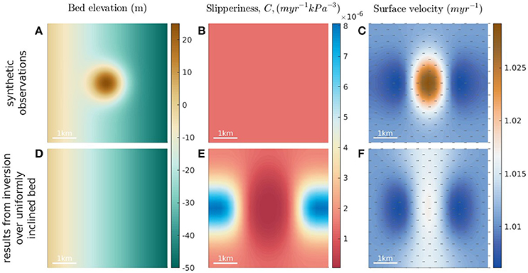
Figure 1. Solutions from a 3D Stokes model set up over a 5 × 5 × 1 km³ inclined slab with periodic boundary conditions. The (A–C) of plots shows the bed perturbation, a constant slipperiness field and then the resultant surface velocity from solving 3D Stokes over this setup. The (D–F) of plots then shows the retrieved slipperiness field and resultant surface velocity when using an inverse method to try and match the surface observations but over a flat bed.

We notice that the model cannot match the surface observations well (i.e., Figures 1C,F show noticeable differences). This is due to the observations being produced from a setup with a perturbation in bed elevation that is not resolved in the domain in which the inversion is conducted. A varying slipperiness field is derived in an attempt to improve the fit to observations. While the slipperiness adjusts in an attempt to compensate for incorrect representation of the bed, the clear structure of the velocity difference does suggests that something is more fundamentally wrong i.e., in this case the basal elevation is incorrect. Ideally the solution should be rejected and the problem identified. However, in reality there are so many irregularities that such solutions would usually be accepted for large-scale ice-sheet inverse models.

This example provides a clear illustration of the need to consider the resolution of bed topography data under PIG, and its influence on results from surface-to-bed inversions. Do synthetic features arise in the derived slipperiness fields if the topography is under-resolved?

4. Modeling Over Pig Tributaries

4.1. The Data

The data used for the inverse modeling consists of bed elevation, surface elevation and surface velocity measurements of PIG. Together with BEDMAP2 bed elevation data (Fretwell et al., 2013), we use newly-acquired high-resolution bed and surface measurements from iSTAR fieldwork (Bingham et al., 2017). This data covers six 10 × 15 km² patches on PIG tributaries; scientists used DELORES (Deep-Looking Radio Echo Sounder) radar (King et al., 2016) over these sites, acquiring twenty-two 15 km radar profiles orthogonal to ice flow, with a 0.5 km spacing between profiles to resolve the bed more fully than it ever had been before.

Figure 2 shows the velocity map of PIG with the areas where the DELORES radar was used marked on. The velocity fields, high-resolution bed data and high-resolution surface data are shown for each site. Many of the features seen in the topography fields are not evident in BEDMAP2 data at all. In this study we choose to focus on iSTARt1 and iSTARt7. This is because of their interesting topographical features; on iSTARt1 there is a defined bump (drumlin-like), the effect of which is reflected in the surface data. Over iSTARt7 the sharp transition in bed elevation is not seen in BEDMAP2; it is completely smoothed out. We want to investigate how much these stark differences in bed affect recovered fields in a surface-to-bed inversion (Figures 3, 4). This will allow us to discuss the importance of the separation of form drag and skin drag. We also have full sets of results from all other sites, which can be found in Appendix 1 (Supplementary Material); we will comment briefly on these as well.

FIGURE 2

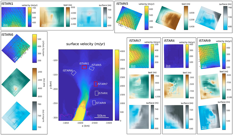
Figure 2. Location of high-resolution data patches on Pine Island Glacier that are used in this study. Results for the two outlined in red are presented in the main part of this paper; results for the other four are in the Appendix (Supplementary Material). For each of the locations we show the velocity (Fahnestock et al., 2016), together with the bed and surface elevation fields (plotted relative to sea level). The thin black dashed box outlines the 10 × 15 km² area over which the DELORES elevation data were collected; the data is merged with BEDMAP2 elevations outside of this box (Fretwell et al., 2013).

FIGURE 3

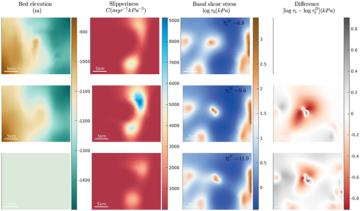
Figure 3. The basal stress field from inversion of surface data over iSTARt1. Three results are shown using three different resolutions of bed elevation data (left column). Mean basal shear stress for each is given.

FIGURE 4

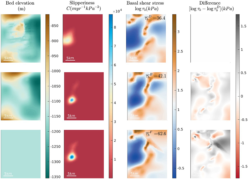
Figure 4. The basal stress field from inversion of surface data over iSTARt7. Three results are shown using three different resolutions of bed elevation data (left column). Mean basal shear stress for each is given.

4.2. Inverse Model Output With Different Bed Resolutions

With the surface velocity and elevation fields in Figure 2, we carry out a surface-to-bed 3D Stokes inversion as detailed in Section 2. This involves minimizing the misfit between the velocity observations and horizontal model output surface velocities to infer the slipperiness field that allows the best fit of observations to data. We carry this out over three different versions of the domain at each site:

1. Bed elevation defined by DELORES high-resolution data (Bingham et al., 2017),

2. Bed elevation defined by BEDMAP2 data (Fretwell et al., 2013),

3. Bed elevation defined as flat.

All use the same high-resolution surface elevation data, as this is easily acquired in comparison with the bed elevation data. This allows us to compare the basal stress fields that result from inverting the surface data over a domain defined with three different bed resolutions. The averaged basal shear stress over each site is also calculated.

Considering first iSTARt1 (Figure 3), it is clear that the maxima and minima in slipperiness/basal stress are present in the same locations whether or not the topography is resolved to a high resolution. The bed is slippy to the side of the grid with the lowest basal elevations. The highest basal shear stress values (i.e., low slipperiness) are at the center of the grid, coinciding with the highest elevation point of the bump. The location of the maximum in basal stress is independent of the resolution of bed topography defining the domain. However, the detail of it does change as the topography is varied. In particular the maximum becomes more locally concentrated when the bump is less fully resolved (evident when looking at the difference fields in the fourth column, which highlight the areas where the form drag is not well resolved without the topography included).

Over iSTARt7 (Figure 4) the results are once again consistent using all three different basal topography options. The maximum in basal shear stress overlies the sharp transition in bed elevation, whether or not the domain is defined with this resolved in the topography. The spatial structure of the derived slipperiness and resulting basal shear stress is consistent with all three topography maps, but the values of the slipperiness and the resulting basal shear stress are not consistent.

Finally, as one further test, we also carry out a surface-to-bed inversion over a larger 100 km² area of PIG. Results are shown in Figure 5 for the case where the domain is defined with bed elevation data from BEDMAP2 (first row) (Fretwell et al., 2013) and the case where the BEDMAP2 data is filtered to only include the long wavelength variation (second row). The high and low slipperiness/basal shear stress areas are found to be in consistent locations. The largest differences in values are found in regions where the most noticeable smoothing has occurred e.g., around the margins of the ice stream.

FIGURE 5

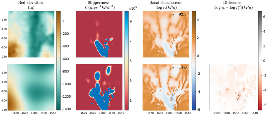
Figure 5. The basal stress field from inversion of surface data over 100 km² of PIG. The result in the top row shows the fields from inversion with BEDMAP2 topography, and in the second row the results are using a smoothed out topography. Mean basal shear stress for each is given.

Furthermore, comparing the mean values of basal shear stress calculated over each site, we see a distinct pattern. The averaged basal shear stress is higher when topography is less fully resolved i.e., ${\overline{\tau }}_b^D<{\overline{\tau }}_b^B<{\overline{\tau }}_b^F$ where the superscripts stand for DELORES, BEDMAP2, and FLAT respectively. This result is true across all six sites (see Figures 1–4 in Appendix 1 Supplementary Material) as well as over the larger domain shown in Figure 5. Mean basal shear stress is lower when the inversion is carried out over the more fully resolved version of the bed. Moreover, the relative change in values of the basal shear stress with the change in topographic detail is interesting as it reflects the relative importance of form drag and skin drag. When there is a significant relative change between cases (e.g., between ${\overline{{\tau }_b}}^B$ and ${\overline{{\tau }_b}}^F$ on iSTARt7 in Figure 4) this suggests that the obstacles unresolved in the smoother topography introduce particularly significant form drag into the problem.

5. Discussion

5.1. Slipperiness and Basal Stress Fields

As described in the previous section, while the spatial patterning of the slipperiness and resultant basal shear stress fields is similar regardless of the resolution of bed topography used, the spatially averaged value of basal shear stress is persistently lower (i.e., higher slipperiness) when more detailed topographic detail is included in the bed elevation field that defines the domain. This is true across all six of the sites where we have the high-resolution topography from DELORES radar measurements.

We propose that this result is due to the form drag that the topography introduces into the problem. Without any topography, all resistance to the flow is through skin drag, which is due to inherent properties of the bed e.g., the presence of water and roughness of sediments. However, topographic variations at the basal boundary induce stresses into the ice, as the ice has to deform around the obstacles. These stresses contribute to the stress balance, providing some of the resistance to the driving stress. It therefore makes sense that the derived skin drag is consistently lower when more detailed bed variations are included in the domain; the form drag transmitted by the bed variations balances more of the driving stress.

5.2. Fit to Observations

Another question we address is how well the surface-to-bed inversion allows the observations to be fitted, and whether this is affected by the resolution of bed elevation data. To consider this question we look at a whole range of results from carrying out the 3D Stokes inversion at each site. The inverse method involves minimizing a cost function, which has a contribution both due to misfit (J_mis) and smoothness of the solution (J_reg) (see Equation 11). We can alter the relative contribution of each; γ² is the ratio of the misfit term to the regularization term in this cost function. The L-curve is a plot of the size of each term at the point that the inversion has converged for a whole range of values of γ. A relative larger regularization term (smaller γ) means enforcing smoothness of the solution is prioritized over decreasing misfit. Misfit values are consequently larger when the regularization term is proportionally larger in the cost function. More details are included in Kyrke-Smith et al. (2017).

Figure 6 shows the L-curves for inversions over both iSTARt1 and iSTARt7 with each different bed topography option. Across all domains the misfit reduces further when using a domain with the bed topography resolved more completely; including more details of the bed allows us to fit to the data better. This is true for results from the inverse model with a whole range of values of the ratio of misfit to regularization in the cost function (the choice of the corresponding parameter, γ, and the robustness of results to its variation is discussed in more detail in Kyrke-Smith et al., 2017). It is encouraging that we see this improved misfit at such local scale; given a model that contains the appropriate physical formulations we would expect a setup more similar to what is producing the observations to allow for a better fit to the surface data.

FIGURE 6

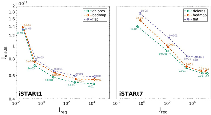
Figure 6. L-curve for results of the model over iSTARt1 and iSTARt7. The value of the regularization term, ${{J}}_{reg1}$, from Equation (11), is plotted against the value of the misfit term, ${{J}}_{mis}$. Values are plotted forresults of the model with a range of values of the coefficient, γ, which governs the relative contribution of regularization and misfit in the cost function. Every point is labeled with the value of γ and the color corresponds to what bed elevation dataset has been used. It is clear that misfit is reduced further by using more fully resolved bed elevation measurements i.e., DELORES measurements rather than BEDMAP2 or a completely smoothed bed.

This result opens up questions about the importance of reducing misfit further for forward predictive modeling. However, it is not something we are able to address conclusively in this paper. Sun et al. (2014) did consider the sensitivity of a dynamic response to bedrock uncertainties and found that the low-frequency noise was of more importance than high frequency noise of the same amplitude. They used a low-aspect ratio model rather than a full Stokes one. It is important that this question is addressed further, particularly in the context of partitioning form and skin drag. While it seems that correctly separating these effects does improve the misfit, it is also important as skin drag is something that can potentially evolve over time, while form drag is static due to it being topographically controlled. Resolving the two correctly will allow us to know what fraction of basal resistance can potentially change over time.

5.3. Comparison With Patterns Observed in Previous Work

Finally we consider how our results compare with Sergienko and Hindmarsh (2013), who saw riblike patterns of very high basal shear stress when carrying out a 3D Stokes surface-to-bed inversion near the grounding line of PIG, keeping the topography fixed using BEDMAP2 bed data (Fretwell et al., 2013). Figure 7 shows results from our model over an area encompassing that shown in Figure 4 in Sergienko and Hindmarsh (2013). There are four plots in Figure 7, each of which is the result of a surface-to-bed inversion with varying proportions of regularization to misfit in the cost function Equation (11). We observe similar features to Sergienko and Hindmarsh (2013), particularly when there is less regularization (i.e., larger γ and more emphasis on reducing the misfit), though the high-shear-stress features are slightly wider (independently of resolution). They are at similar angles and locations, though not identical.

FIGURE 7

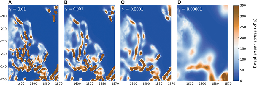
Figure 7. The basal stress field from inversion of surface data over a 40 × 60 km² area of the domain, corresponding to the area by the grounding line over which Sergienko and Hindmarsh (2013) observed riblike patterns of very high basal shear stress. (A–D) are results with four different amounts of regularization applied to the inversion (the value of γ in Equation 11 for each is given). The amount of regularisation increases from A–D.

Increasing the amount of regularization in the cost function suppresses the high-frequency features (see how the plots change as γ decreases in Figure 7). Such an increase in smoothness is expected to be concurrent with the surface observations being less well-matched. In this case the decrease in velocity misfit as a result of enforcing more smoothness on the solution is not particularly significant: misfit increases by 0.3% as γ decreases from 10⁻² to 10⁻³, 0.4% as γ decreases from 10⁻³ to 10⁻⁴ and 1.4% as γ decreases from 10⁻⁴ to 10⁻⁵. The latter is the most significant, and does occur at the point where the high frequency variations are almost completely suppressed. However, we suggest that the presence of the riblike features are not a absolute necessity for a good fit to velocity data, and that more work needs to be done to establish their robustness. We also suggest that areas where ribs are identified from inverse modeling should be prioritized as locations for high resolution bed elevation surveys; inverse methods can recover a mixture of unresolved form drag combined with skin friction effects (as seen in the “toy” problem illustrated in Figure 1E) and it would seem sensible to test whether any of the high shear stress patterns may arise due to unresolved form drag.

6. Conclusions

Previous work has considered the transfer of basal perturbations to the surface and attempted to quantify the wavelengths that are of importance (e.g., Gudmundsson, 1997, 2003; Gudmundsson et al., 1998; Schoof, 2002). In this paper we considered a related question: given high resolution surface observations, how robust are predictions of basal slipperiness to the resolution of the bed elevation data on PIG? We addressed this by looking at the effect of including small-scale bed features when carrying out 3D Stokes surface-to-bed inversions. While such variations are not necessarily on the lengthscales that transfer information to the surface, they may still introduce significant form drag into the problem.

Results of the inverse study showed that the structure of spatial variations in recovered slipperiness is not affected by how finely the topography is resolved (see Figures 3–5). This is not altogether surprising given that transfer studies suggest that both bed and slipperiness variations on small scales do not significantly affect surface velocities. There is therefore no reason for the spatial variability of slipperiness to change significantly when the bed is known to a higher resolution. However, we did find consistently lower mean values of basal shear stress over each site when incorporating the high-resolution bed elevation data into the domain. We suggested that this is because small bed obstacles are more efficient at causing form drag (e.g., Schoof, 2002); more of the driving stress is therefore resisted by the form drag resulting from ice deforming around the topography included in the model. The skin drag derived from the inversion is consequently noticeably lower when more detail is included in the bed. Furthermore, we obtained a better fit to surface velocities using the more accurate bed-topography data set (Section 5.2). This is expected if the model is correct for the system, and was found to be true across a range of regularization to misfit ratios. Finally, we also reproduced high-shear-stress, riblike features like those seen in Sergienko and Hindmarsh (2013). They were especially clear when only a small amount of regularization was applied in the inverse model (Figure 7), and could be suppressed by applying more regularization to the problem. Nevertheless, while the misfit was not affected too significantly, the L-curve approach did suggest that the correct amount of regularization is in the region where we recovered the high-basal-stress features.

In conclusion, we suggest that values of basal shear stress derived from a surface-to-bed inverse approach need to be interpreted with caution as they can include drag which is due to the unresolved topography rather than inherent bed and sediment conditions. While we have not explicitly investigated the consequences of this for forward modeling, we believe it could be an important consideration for predictive models. Separation of form and skin drag would be particularly important when including evolution of basal conditions in a model, as the time-independent effects of form drag should be resolved separately to the time-dependent skin drag. Without access to the highest-resolution bed elevation data everywhere, it would seem that inverting simultaneously for both bed topography and basal slipperiness (Raymond and Gudmundsson, 2009; Raymond Pralong and Gudmundsson, 2011) might be the most sensible approach to take to address the problem.

Author Contributions

The work was carried out by TK-S at BAS, with regular help from GG in the form of discussion and advice. PF helped set up the numerical model that is used in the paper.

Conflict of Interest Statement

The authors declare that the research was conducted in the absence of any commercial or financial relationships that could be construed as a potential conflict of interest.

Acknowledgments

We would like to thank Rob Arthern for useful conversations while preparing this manuscript, Rob Bingham for giving us access to the radar data in advance of publication, and the reviewers for helpful and constructive comments during the review process. Data will be available on the NERC/iSTAR GIS site, http://gis.istar.ac.uk. This work was supported by funding from the UK Natural Environment Research Council's iSTAR Programme and NERC Grant Number NE/J005754/1. Farrell is supported by EPSRC grant EP/K030930/1.

Supplementary Material

The Supplementary Material for this article can be found online at: https://www.frontiersin.org/articles/10.3389/feart.2018.00033/full#supplementary-material

References

Alnæs, M. S., Blechta, J., Hake, J., Johansson, A., Kehlet, B., Logg, A., et al. (2015). The FEniCS Project version 1.5. Arch. Num. Softw. 3. doi: 10.11588/ans.2015.100.20553

CrossRef Full Text | Google Scholar

Balise, M. J., and Raymond, C. F. (1985). Transfer of basal sliding variations to the surface of a linearly viscous glacier. J. Glaciol. 31, 308–318. doi: 10.1017/S002214300000664X

CrossRef Full Text | Google Scholar

Bingham, R. G., King, E. C., Davies, D., Cornford, S. L., Smith, A. M., Arthern, R. J., et al. (2017). Diverse landscapes beneath Pine Island Glacier influence ice flow. Nat. Communs. 8:1618. doi: 10.1038/s41467-017-01597-y

PubMed Abstract | CrossRef Full Text | Google Scholar

Budd, W. F. (1970). Ice flow over bedrock perturbations. J. Glaciol. 90, 29–48. doi: 10.3189/S0022143000026770

CrossRef Full Text | Google Scholar

Budd, W. F., Keage, P. L., and Blundy, N. A. (1979). Empirical studies of ice sliding. J. Glaciol. 23, 157–170. doi: 10.1017/S0022143000029804

CrossRef Full Text | Google Scholar

De Rydt, J., Gudmundsson, G. H., Corr, H. F., and Christoffersen, P. (2013). Surface undulations of Antarctic ice streams tightly controlled by bedrock topography. Cryosphere 7, 407–417. doi: 10.5194/tc-7-407-2013

CrossRef Full Text | Google Scholar

Durand, G., Gagliardini, O., Favier, L., Zwinger, T., and le Meur, E. (2011). Impact of bedrock description on modeling ice sheet dynamics. Geophys. Res. Lett. 38:L20501. doi: 10.1029/2011GL048892

CrossRef Full Text | Google Scholar

Fahnestock, M., Scambos, T., Moon, T., Gardner, A., Haran, T., and Klinger, M. (2016). Rapid large-area mapping of ice flow using Landsat 8. Remote Sens. Environ. 185, 84–94. doi: 10.1016/j.rse.2015.11.023

CrossRef Full Text | Google Scholar

Farinotti, D., Huss, M., Bauder, A., Funk, M., and Truffer, M. (2009). A method to estimate the ice volume and ice-thickness distribution of alpine glaciers. J. Glaciol. 55, 422–430. doi: 10.3189/002214309788816759

CrossRef Full Text | Google Scholar

Farrell, P. E., Ham, D. A., Funke, S. W., and Rognes, M. E. (2013). Automated derivation of the adjoint of high-level transient finite element programs. SIAM J. Sci. Comp. 35, C369–C393. doi: 10.1137/120873558

CrossRef Full Text | Google Scholar

Favier, L., Durand, G., Cornford, S. L., Gudmundsson, G. H., Gagliardini, O., Gillet-Chaulet, F., et al. (2014). Retreat of Pine Island Glacier controlled by marine ice-sheet instability. Nat. Clim. Change 4, 117–121. doi: 10.1038/nclimate2094

CrossRef Full Text | Google Scholar

Fretwell, P., Pritchard, H. D., Vaughan, D. G., Bamber, J. L., Barrand, N. E., Bell, R., et al. (2013). Bedmap2: improved ice bed, surface and thickness datasets for Antarctica. Cryosphere 7, 375–393. doi: 10.5194/tc-7-375-2013

CrossRef Full Text | Google Scholar

Fowler, A. C. (2010). Weertman, Lliboutry and the development of sliding theory. J. Glaciol. 56, 965–972. doi: 10.3189/002214311796406112

CrossRef Full Text | Google Scholar

Glen, J. W. (1955). The creep of polycrystalline ice. Proc. R. Soc. A. 228, 519–538. doi: 10.101098/rspa.1955.0066

CrossRef Full Text | Google Scholar

Goldberg, D. N., and Heimbach, P. (2013). Parameter and state estimation with a time-dependent adjoint marine ice sheet model. Cryosphere 7, 1659–1678. doi: 10.5194/tc-7-1659-2013

CrossRef Full Text | Google Scholar

Gudmundsson, G. H. (1997). Basal-flow characteristics of a non-linear flow sliding frictionless over strongly undulating bedrock. J. Glaciol. 43, 80–89. doi: 10.1017/S002214300000283

CrossRef Full Text | Google Scholar

Gudmundsson, G. H., Raymond, C. F., and Bindschadler, R. (1998). The origin and longevity of flow stripes on Antarctic ice streams. Ann. Glaciol. 27, 145–152. doi: 10.3189/1998AoG27-1-145-152

CrossRef Full Text | Google Scholar

Gudmundsson, G. H. (2003). Transmission of basal variability to a glacier surface. J. Geophys. Res. 108:B5. doi: 10.1029/2002JB002107

CrossRef Full Text | Google Scholar

Gudmundsson, G. H., and Raymond, M. (2008). On the limit to resolution and information on basal properties obtainable on surface data on ice streams. Cryosphere 2, 167–178. doi: 10.5194/tc-2-167-2008

CrossRef Full Text | Google Scholar

Iverson, N. R., and Zoet, L. K. (2015). Experiments on the dynamics and sedimentary products of glacier slip. Geomorphology 244, 121–134. doi: 10.1016/j/geomorph.2015.03.027

CrossRef Full Text | Google Scholar

King, E. C., Pritchard, H. D., and Smith, A. M. (2016), Subglacial landforms beneath Rutford Ice Stream, Antarctica: detailed bed topography from ice-penetrating radar. Earth Syst. Sci. Data 8, 151–158. doi: 10.5194/essd-8-151-2016

CrossRef Full Text | Google Scholar

Konrad, H., Gilbert, L., Cornford, S. L., Payne, A., Hogg, A., Muir, A., et al. (2017), Uneven onset pace of ice-dynamical imbalance in the Amundsen Sea Embayment, West Antarctica. J. Geophys. Res. 44, 910–918. doi: 10.1002/2016GL070733.

CrossRef Full Text | Google Scholar

Kyrke-Smith, T. M., Gudmundsson, G. H., and Farrell, P. E. (2017). Can seismic observations of bed conditions on ice streams help constrain parameters in ice flow models? J. Geophys. Res. 122, 2269–2282. doi: 10.1002/2017JF004373

CrossRef Full Text | Google Scholar

Langdon, G., and Raymond, C. F. (1978). Numerical calculation of adjustment of a glacier surface to perturbations of ice thickness. Mater. Glyatsiol. Issled. Khron. Obsuzhdeniya 32, 233–239.

Li, H., Ng, F., Li, Z., Qin, D., and Cheng, G. (2012). An extended perfect-plasticity method for estimating ice thickness along the flow line of mountain glaciers. J. Geophys. Res. 117:F01020. doi: 10.1029/2011JF002104

CrossRef Full Text | Google Scholar

Lliboutry, L. (1968). General theory of subglacial cavitation and sliding of temperate glaciers. J. Glaciol. 7, 21–58. doi: 10.3198/1968JoG7-49-21-58

CrossRef Full Text | Google Scholar

Leguy, G. R., Asay-Davis, X. S., and Lipscomb, W. H. (2014). Parameterization of basal friction near grounding lines in a one-dimensional ice sheet model. Cryosphere 8, 1239–1259. doi: 10.5194/tc-8-1239-2014

CrossRef Full Text | Google Scholar

Logg, A., Mardal, K. A., and Wells, G. N. (2012). Automated Solution of Differential Equations by the Finite Element Method. Berlin; Heidelberg: Springer.

Google Scholar

Macayeal, D. R. (1992). The basal stress distribution of Ice Stream E, Antarctica, inferred by control methods. J. Geophys. Res. 97, 595–603. doi: 10.1029/91JB02454

CrossRef Full Text | Google Scholar

Macayeal, D. R. (1993). A tutorial on the use of control methods in ice-sheet modeling. J. Glaciol. 39, 91–98. doi: 10.3198/1993JoG39-131-91-98

CrossRef Full Text | Google Scholar

Martin, N., and Monnier, J. (2014). Adjoint accuracy for the full Stokes ice flow model: limits to the transmission of basal friction variability to the surface. Cryosphere 8, 721–741. doi: 10.5194/tc-8-721-2014

CrossRef Full Text | Google Scholar

Morlighem, M., Rignot, E., Seroussi, H., Larour, E., Ben Dhia, H., and Aubry, D. (2010). Spatial patterns of basal drag inferred using control methods from a full-Stokes and simpler models for Pine Island Glacier, West Antarctica. Geophys. Res. Lett. 37:L14502. doi: 10.1029/2010GL043853

CrossRef Full Text | Google Scholar

Morlighem, M., Rignot, E., Seroussi, H., Larour, E., Ben Dhia, H., and Aubry, D. (2011). A mass conservation approach for mapping glacier ice thickness. Geophys. Res. Lett. 38:L19503. doi: 10.1029/2011GL048659

CrossRef Full Text | Google Scholar

Morlighem, M., Seroussi, H., Larour, E., and Rignot, E. (2013). Inversion of basal friction in Antarctica using exact and incomplete adjoints of a higher-order model. J. Geophys. Res. 118, 1746–1753. doi: 10.1002/jgrf.20125

CrossRef Full Text | Google Scholar

Mouginot, J., Rignot, E., and Scheuchl, B. (2014). Sustained increase in ice discharge from the Amundsen Sea Embayment, West Antarctica, from 1973 to 2013. Geophys. Res. Lett. 41, 1576–1584. doi: 10.1002/2013GL059069

CrossRef Full Text | Google Scholar

Nias, I. J., Cornford, S. L., and Payne, A. J. (2016). Contrasting the modelled sensitivity of the Amundsen Sea Embayment ice streams. J. Glaciol. 62, 552–562. doi: 10.1002/jog.2016.40

CrossRef Full Text | Google Scholar

Nye, J. F. (1959). The motion of ice sheets and glaciers. J. Glaciol. 3, 493–507.

Google Scholar

Petra, N., Zhu, H., Stadler, G., Hughes, T. J. R., and Ghattas, O. (2012). An inexact Gauss-Newton method for inversion of basal sliding and rheology parameters in a nonlinear Stokes ice sheet model. J. Glaciol. 58, 889–903. doi: 10.3189/2012JoG11J182

CrossRef Full Text | Google Scholar

Raymond, M. J., and Gudmundsson, G. H. (2005). On the relationship between surface and basal properties on glaciers, ice sheets and ice streams. J. Geophys. Res. 110:B08411. doi: 10.1029/2005JB003681

CrossRef Full Text | Google Scholar

Raymond, M. J., and Gudmundsson, G. H. (2009). Estimating basal properties of ice streams from surface measurements: a nonlinear Bayesian inverse approach applied to synthetic data. Cryosphere 3, 265–278. doi: 10.5194/tc-3-265-2009

CrossRef Full Text | Google Scholar

Raymond Pralong, M., and Gudmundsson, G. H. (2011). Bayesian estimation of basal conditions on Rutford Ice Stream, West Antarctica, from surface data. J. Glaciol. 57, 315–324. doi: 10.3189/002214311796406004

CrossRef Full Text | Google Scholar

Rignot, E., Mouginot, J., Morlighem, M., Seroussi, H., and Scheuchl, B. (2014). Widespread, rapid grounding line retreat of Pine Island, Thwaites, Smith and Kohler glaciers, West Antarctica, from 1992 to 2011. Geophys. Res. Lett. 41, 3502–3509. doi: 10.1002/2014GL060140

CrossRef Full Text | Google Scholar

Ritz, C., Edwards, T. L., Durand, G., Payne, A. J., Peyaud, V., and Hindmarsh, R. C. A. (2015). Potential sea-level rise from Antarctic ice-sheet instability constrained by observations. Nature 528, 115–118. doi: 10.1038/nature16147

PubMed Abstract | CrossRef Full Text | Google Scholar

Schoof, C. (2002). Basal perturbations under ice streams: form drag and surface expression. J. Glaciol. 48, 407–416. doi: 10.3189/172756502781831269

CrossRef Full Text | Google Scholar

Schoof, C. (2007). Ice sheet grounding line dynamics: Steady states, stability, and hysteresis. J. Geophys. Res. 112:F03S28. doi: 10.1029/2006JF000664

CrossRef Full Text | Google Scholar

Sergienko, O. V., Bindschadler, R. A., Vornberger, P. L., and Macayeal, D. R. (2008). Ice stream basal conditions from block-wise surface data inversion and simple regression models of ice stream flow: application to Bindschadler Ice Stream. J. Geophys. Res. 113:F04010. doi: 10.1029/2008JF001004

CrossRef Full Text | Google Scholar

Sergienko, O. V., and Hindmarsh, R. C. A. (2013). Regular patterns in frictional resistance of ice-stream beds seen by surface data inversion. Science 342, 1086–1089. doi: 10.1126/science.1243903

PubMed Abstract | CrossRef Full Text | Google Scholar

Seroussi, H., Morlighem, M., Rignot, E., Mouginot, J., Larour, E., Schodlok, M., et al. (2014). Sensitivity of the dynamics of Pine Island Glacier, West Antarctica, to climate forcing for the next 50 years. Cryosphere 8, 1699–1710. doi: 10.5194/tc-8-1699-2014

CrossRef Full Text | Google Scholar

Smith, J. A., Andersen, T. J., Shortt, M., Gaffney, A. M., Truffer, M., Stanton, T. P., et al. (2017). Sub-ice-shelf sediments record history of twentieth-century retreat of Pine Island Glacier. Nature 541, 77–80. doi: 10.1038/nature20136

PubMed Abstract | CrossRef Full Text | Google Scholar

Sun, S., Cornford, S. L., Lui, Y., and Moore, J. C. (2014). Dynamic response of Antarctic ice shelves to bedrock uncertainty. Cryosphere 8, 1561–1576. doi: 10.5194/tc-8-1561-2014

CrossRef Full Text | Google Scholar

Van Pelt, W. J. J., Oerlemans, J., Reijmer, C. H., Pettersson, R., Pohjola, V. A., Isaksson, E., et al. (2013). An iterative inverse method to estimate basal topography and initialize ice flow models. Cryosphere 7, 987–1006. doi: 10.5194/tc-7-987-2013

CrossRef Full Text | Google Scholar

Weertman, J. (1957). On the sliding of glaciers. J. Glaciol. 3, 33–38. doi: 10.1002/2016GL069937

CrossRef Full Text | Google Scholar

Williams, C. R., Hindmarsh, R. C. A., and Arthern, R. J. (2012). Frequency response of ice streams. Proc. R. Soc. A 468, 3285–3310. doi: 10.1098/rspa.2012.0180

PubMed Abstract | CrossRef Full Text | Google Scholar

Wingham, D. J., Wallis, D. W., and Shepherd, A. (2009). Spatial and temporal evolution of Pine Island Glacier thinning, 1995–2006. Geophys. Res. Lett. 36:L17501. doi: 10.1029/2009GL039126

CrossRef Full Text | Google Scholar