Advantages of Measuring the Q Stokes Parameter in Addition to the Total Radiance I in the Detection of Absorbing Aerosols

1. Introduction

The Moderate Resolution Imaging Spectroradiometer (MODIS) is a scientific instrument that was launched into Earth orbit by NASA in 1999 on board the Terra satellite, and in 2002 on board the Aqua satellite. The instruments measure total radiances at varying spatial resolutions (2 bands at 250 m, 5 bands at 500 m, and 29 bands at 1 km) in 36 spectral bands ranging in wavelength from 0.4 μm to 14.4 μm. Together the two instruments image the entire Earth every 1–2 days. They are designed to provide information about large-scale global dynamics including changes in Earth's cloud cover, radiation budget, and processes occurring in the oceans, on land, and in the lower atmosphere. The MEdium Resolution Imaging Spectrometer (MERIS) was deployed on board the European Space Agency's Envisat platform from 2002 until 2012. The MERIS instrument employs spectrometers that measure reflected sunlight in several spectral bands between 390 and 1,040 nm. Its main purpose was to study/monitor the health of open ocean and coastal water bodies. The success of the MODIS and MERIS spectroradiometers was followed up by VIIRS, OLCI (by ESA), and SGLI (by JAXA). But apart from SGLI, which has two bands that can measure polarization, these instruments only measure the total radiance, or the I Stokes parameter.

In this study we asked a simple question: what if MODIS (or MERIS) could measure polarization? To be more specific, what advantage would be obtained from measuring the Q = I_∥ − I_⊥ Stokes parameter in addition to the total radiance (or intensity) I = I_∥ + I_⊥? In remote sensing, the goal is to retrieve atmosphere/surface parameters from measurements by solving the so-called inverse problem.

Currently, in order to invert the total radiance measured by MODIS, traditional methods rely on two steps: (i) an “atmospheric correction” to obtain the surface reflectance (over land) or the remote sensing reflectance (over water), and (ii) an inversion of the signal so obtained to retrieve land (water) parameters (Gordon and Wang, 1994; Gordon, 1997). Advantages of the traditional method are that it is (i) operationally fast, (ii) relatively simple to implement, and (iii) works well in many scenarios. Two disadvantages of the traditional approach are that the simplified two-step approach can lead to retrieval inaccuracies and/or negative water-leaving radiances, and that error budget calculations become cumbersome. Alternatively, it has been shown that simultaneous retrieval of atmosphere/ocean properties using statistically-based optimal estimation techniques can improve retrieval accuracy and also allow for adequate error budget calculations (Stamnes et al., 2005; Spurr et al., 2007; Li et al., 2008). The disadvantages of statistically-based techniques are that they are operationally slow and relatively complex to implement.

However, even with optimal estimation, remote sensing measurements that rely only on the total radiance are fraught with uniqueness problems. In order to retrieve information about absorbing aerosols over coastal waters as well as over bright targets such as snow and ice, polarization measurements are very important, because it is difficult to infer the aerosol single-scattering albedo from spectrometers such as MERIS and MODIS that measure the total radiance only. Accurate retrieval of aerosol vertical location and single-scattering albedo is important for calculating warming/cooling rates, for ocean color remote sensing, and to retrieve surface properties of bright targets like snow and ice. Aerosol vertical location is also important for understanding atmospheric circulation, transport and evolution of aerosols, including changes in single-scattering albedo.

Some previous studies have looked into the use of polarization. For example, Hasekamp et al. (2011), while looking at multi-angular measurements, considered also the case of adding polarization to I-only retrievals and found improved agreement with ground-based (AERONET) data. Di Noia et al. (2017) found that use of a neural network to provide an initial guess for an iterative algorithm led to a decrease in processing time and an increase in the number of converged retrievals. And neural networks have been used to directly retrieve products, e.g., ozone column amounts from ground-based irradiance measurements (Fan et al., 2014) or satellite water-leaving radiances (Fan et al., 2017), and have also been used with optimal estimation, e.g., retrieval of snow products from ground-based total radiance measurements (Tanikawa et al., 2015).

Given this background, the goal of the study is to use a vector radiative transfer model for the coupled atmosphere-surface system in conjunction with optimal estimation to investigate how polarization measurements can be used to overcome uniqueness problems associated with total radiance-only retrieval of aerosol parameters. This approach can also be used to explore how future instruments, which would measure also the Stokes parameters Q and U in addition to the total radiance I, may enhance our ability to retrieve accurate aerosol parameters over turbid coastal waters and bright targets like snow and ice.

Although we focus solely on the Q component in this study, the U component is also important except in the principal plane. For example, POLDER-1 on ADEOS, which was in operation from October 1996 to June 1997, by NASDA (now JAXA), was the first satellite sensor to measure Stokes components I, Q, and U. The POLDER-2 sensor on ADEOS-II (Leroy and Lifermann, 2000), and POLDER-3 (Herman et al., 2005) on PARASOL have been operational in space. It is also noteworthy that the JAXA SGLI sensor on GCOM-C also measures I, Q, and U (Imaoka et al., 2010), and was successfully launched in late December of 2017 and will begin operation in Spring of 2018.

2. Study Design

The goal is to explore the feasibility of retrieving the optical depth at a reference wavelength (τ_λref), the (absorbing) fine mode optical depth fraction (f_τa), and the vertical location (z_i) of the aerosol by employing a bimodal mixture of lognormal aerosol size distributions. One population is assumed to consist of non-absorbing coarse mode (sea-salt type) particles and the other one of absorbing fine mode (soot type) particles.

The SeaDAS aerosol models (see Figure 1) are based on AERONET data (Ahmad et al., 2010), and they include a non-absorbing coarse mode (sea-salt) particle type as well a weakly absorbing fine mode particle component consisting of an external mixture of 0.5% soot particles and 99.5% dust particles (Shettle and Fenn, 1979). In order to create an aerosol model that includes significant absorption, we modified the fine mode of the SeaDAS aerosol model to use 100% soot particles.

FIGURE 1

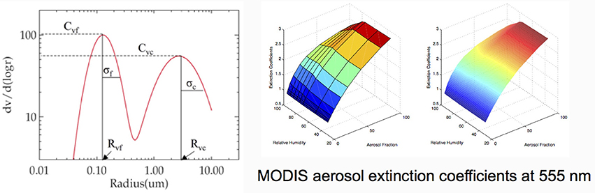
Figure 1. SeaDAS bimodal aerosol model (Ahmad et al., 2010). (Left) Size distributions of the fine and coarse aerosol modes which are assumed to be log-normally distributed in volume space with a fixed width of 0.437 for the fine mode and 0.672 for the coarse mode. (Middle) The ten different aerosol fine mode fractions in volume space: f_V = 0, 1, 2, 5, 10, 20, 30, 50, 80, 95%, and eight different relative humidities: 30, 50, 70, 75, 80, 85, 90, 95%. We used the SeaDAS median radius at a relative humidity of 70% for this study. Thus the fine mode mean radius was 90 nm, and the coarse mode median radius was 755 nm. And for this study the fine mode complex refractive index was set to that of 100% soot to represent an absorbing particle. (Right) “Continuum” of models obtained by interpolation between the discrete SeaDAS models. Note that the aerosol fine mode fraction in volume space was retrieved in this study, except it was expressed in terms of the fine mode optical depth fraction.

Thus, we have a bimodal aerosol mixture consisting of a total of N = N_a + N_c particles per unit volume in a layer of thickness Δz, where N_a and N_c are concentrations of absorbing fine mode and non-absorbing coarse mode particles. Computation of aerosol inherent optical properties (IOPs) involves definitions of σ_n,i = scattering cross section, α_n,i = absorption cross section, and k_n,i = σ_n,i + α_n,i = extinction cross section, where i = a stands for “absorbing fine mode,” and i = c stands for “non-absorbing coarse mode.”

Standard mixing formulas (weighted by number concentrations) are used to combine the absorption and scattering cross sections as well as the moments of the scattering phase matrix elements (Stamnes et al., 2017). Hence, the IOPs of the mixture are (subscript m stands for mixture):

$\begin{array}{l}\Delta {\tau }_m=k_m\Delta z=\left[N_a{k}_{n,a}+N_c{k}_{n,c}\right]\Delta z=\left[k_a+k_c\right]\Delta z\\ =\Delta {\tau }_a+\Delta {\tau }_c,& (1)\end{array}$

$\begin{array}{ll}{N}_a=f_{N}N,N_c=(1-f_N)N,N=N_a+N_c,& (2)\end{array}$

$\begin{array}{ll}{k}_a=k_{n,a}{N}_a,k_c=k_{n,c}{N}_c,k_m=k_a+k_c,& (3)\end{array}$

$\begin{array}{ll}{f}_{{\tau }_a}=\frac{\Delta {\tau }_a}{\Delta {\tau }_m},& (4)\end{array}$

$\begin{array}{l}{\varpi }_m=\frac{{\varpi }_a{k}_a+{\varpi }_c{k}_c}{k_m}=\frac{f_N{\varpi }_a{k}_{n,a}+(1-f_N){\varpi }_c{k}_{n,c}}{f_N{k}_{n,a}+(1-f_N)k_{n,c}}\\ ={\varpi }_a{f}_{{\tau }_a}+{\varpi }_c{f}_{{\tau }_a}\frac{\Delta {\tau }_c}{\Delta {\tau }_a},& (5)\end{array}$

$\begin{array}{ll}{\chi }_{m,\ell }=\frac{f_N{\varpi }_a{k}_{n,a}{\chi }_{a,\ell }+(1-f_N){\varpi }_c{k}_{n,c}{\chi }_{c,\ell }}{f_N{\sigma }_{n,a}+(1-f_N){\sigma }_{n,c}},& (6)\end{array}$

where Δτ_m = layer optical depth; k_m = extinction coefficient; ϖ_m = single-scattering albedo; χ_{m, ℓ} = phase function Legendre polynomial expansion coefficient; f_N = fraction of fine mode (absorbing) particles in number-density space, f_τa = optical depth fraction of fine mode absorbing aerosols (hereafter referred to as “fine mode fraction”). For each element of the scattering phase matrix, a mixing rule similar to Equation (6) is applied.

For simplicity, we assumed that the underlying ocean consisted of pure sea water, although in future work embedded impurities could be added.

To simplify the study we created a synthetic dataset by randomly varying the following input parameters to our vector radiative transfer code (C-VDISORT, Cohen et al., 2013): {θ₀, θ, Δϕ, τ_λref, f_τa, z_i(i = 0, 1)}, where θ₀ is the solar zenith angle (fixed at 30°), θ is the sensor polar viewing angle, and Δϕ is the sun-sensor difference in azimuth angle. The sensor viewing angle range is θ: [30°, 60°], Δϕ: [120°, 150°]. Our retrieval parameters (RPs) are represented by the set {τ_λref, f_τa, z_i(i = 0, 1)}, where τ_λref is the aerosol optical depth at λ_ref with range [0.001, 0.5]; f is the bimodal aerosol fraction with range [0, 1]; and z_i(i = 0, 1) is the vertical location of aerosols in either layer z₀ [0, 2 km] or layer z₁ [2, 4 km], represented by an integer value z₀ = 1 and z₁ = 3.

Our question may now be restated as: can aerosol optical depth, fine mode fraction, and vertical location, i.e., {τ_λref, f_τa, z_i(i = 0, 1)}, be inferred from synthetic “MODIS” data of I and Q?

3. Neural Network Fast Forward Model and Neural Network based First Guess by Direct Inversion

The fast radiative transfer forward model is based on radial basis functions generated by a neural network in order to speed-up the forward computations and thereby the inversion. The forward model (C-VDISORT) computations are normally, the most time-consuming step by far in the inversion process. However, we found it possible to increase the speed on the order of 1,000 times or more by using a synthetic dataset produced by C-VDISORT to train a Radial Basis Functions Neural Network (RBF-NN) (Broomhead and Lowe, 1988). This speed-up enables processing of imaging data from spectroradiometers like MODIS and MERIS that collect millions of pixels per image. The RBF-NN forward model replaces the C-VDISORT forward model (thousands of lines of code) with the following single equation (Stamnes and Stamnes, 2015):

$\begin{array}{ll}{p}_i={\displaystyle \sum _{j=1}^N}{a}_{ij}exp[-b^2{\displaystyle \sum _{k=1}^{N_{in}}}{(R_k-c_{jk})}^2]+d_i& (7)\end{array}$

where N is the total number of neurons and N_in is the number of input parameters. The Jacobians K, needed in the optimal estimation (see Equation 10 below), are obtained by calculating the partial derivatives with respect to the retrieval parameter R_k:

$\begin{array}{l}{K}_k=\frac{\partial p_i}{\partial R_k}=-2b^2(c_{jk}-R_k)\\ \times {\displaystyle \sum _{j=1}^N}{a}_{ij}exp[-b^2{\displaystyle \sum _{k=1}^{N_{in}}}{(c_{jk}-R_k)}^2].& (8)\end{array}$

The training of the RBF-NN determines the coefficients a_ij, b, c_jk, and d_i appearing in Equations (7) and (8). Here we should note that if the goal is to retrieve the state parameters directly, e.g., from measurements of TOA total radiances, then the input parameters R_k in Equation (7) would be the TOA Stokes parameters at the desired wavelengths as well as the solar/viewing geometry, and the output parameters p_i would be the desired retrieval (state) parameters (Stamnes and Stamnes, 2015). In this study we use this approach to obtain a neural network based first guess as the starting point for a nonlinear optimal estimation (see Equation 10 below). We will compare the neural network based first guess with a “naive” first guess which is fixed to be close to the midpoint of the range of retrieval parameters, and represents little a priori knowledge about the system.

On the other hand, if the goal is to use the RBF-NN as a fast interpolator to obtain the TOA Stokes parameters and associated Jacobians (see Equation 8), then the input parameters R_k are the state parameters and the solar/viewing geometry, and the output parameters p_i are the TOA Stokes parameters (Stamnes and Stamnes, 2015). Since our primary goal in this study was to use the RBF-NN as a fast forward model, the input parameters R_k in Equation (7) are the state parameters and the solar/viewing geometry, and the output parameters p_i are the desired TOA Stokes parameters, I and Q at the nine MODIS VIS channels centered at 412, 443, 488, 531, 547, 667, 678, 748, and 869 nm.

A training dataset of 20,000 randomly generated state vectors was used to train the RBF-NN forward model. We added random Gaussian measurement noise with a standard deviation of 3% to this training dataset, and trained the inverse neural network to go from the TOA I and Q radiances to the retrieval parameters. We then constructed a different “truth” dataset of 20,000 scenes, to which we also added 3% random Gaussian noise. Having two separate datasets for training and truth helps to test that the neural network training was sufficiently robust.

In Figure 2 we compare C-VDISORT and RBF-NN results for the Stokes parameter I. A similar comparison for the Stokes parameter Q is provided in Figure 3. The performance of the neural network is evaluated statistically by direct comparison to C-VDISORT for randomly-selected inputs within the training range. This comparison shows that the correlations exceed 0.999 for all nine channels for the I as well as the Q Stokes component.

FIGURE 2

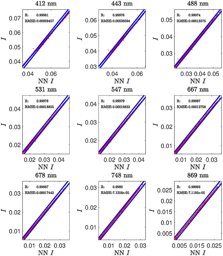
Figure 2. Comparison of RBF-NN forward model results for I with C-VDISORT results for the nine MODIS VIS channels used in this study.

FIGURE 3

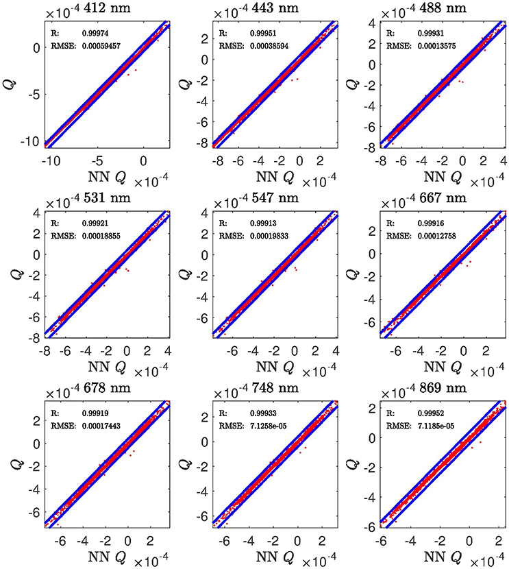
Figure 3. Comparison of RBF-NN forward model results for Q with C-VDISORT results for the nine MODIS VIS channels used in this study.

4. Optimal Estimation/Inverse Model

Our goal is to use C-VDISORT/RBF-NN and Optimal Estimation/Levenberg-Marquardt (OE/LM) inversion to explore the retrieval feasibility. We assume that the state vector consists of three aerosol parameters: the optical depth τ_λref at λ_ref, the (absorbing) fine mode fraction f_τa, and the vertical location z_i of the aerosols. Hence, the state vector becomes:

$\begin{array}{ll}\text{x}=\{{\tau }_{{\lambda }_{ref}},f_{{\tau }_a},z_i(i=0\mathrm{\text{ or }}1)\}.& (9)\end{array}$

We employed OE/LM inversion to find the “optimum” result from the simulated measurements of I and Q. Hence, in each iteration the next estimate of the state vector was given by Rodgers (2000) and Stamnes and Stamnes (2015)

$\begin{array}{l}{\text{x}}_{i+1}={\text{x}}_i+{[(1+{\gamma }_i){\text{S}}_a^{-1}+{\text{K}}_i^T{\text{S}}_m^{-1}{\text{K}}_i]}^{-1}\\ \times \{{\text{K}}_i^T{\text{S}}_m^{-1}({\text{y}}_m-{\text{y}}_i)-{\text{S}}_a^{-1}({\text{x}}_i-{\text{x}}_a)\}& (10)\end{array}$

where y_m and y_i are actual and simulated measurements, and x_a and S_a are the a priori state vector and the covariance matrix, respectively. x_i+1 and x_i are the state vectors at the current and the previous iterations. S_m is the measurement error covariance matrix, which was set equal to the squares of 3% of the Stokes parameters to be consistent with the measurement error used in this study. As the Levenberg-Marquardt (LM) parameter γ_i → 0, Equation (10) becomes a standard Gauss-Newton optimal estimation whereas for a large value of γ_i Equation (10) tends to the steepest descent method. Note that the fast C-VDISORT/RBF-NN forward model returns simulated Stokes parameters (y_i → p_i, Equation 7) and Jacobians K_i, (Equation 8) required to update the state vector estimate (x_i) using Equation (10).

It should be emphasized that the results reported in this paper are based on synthetic data generated for MODIS channels centered at 412, 443, 488, 531, 547, 667, 678, 748, and 869 nm. Although, optical depth retrievals are reported at only the reference wavelength λ_ref = 869 nm, results at other wavelengths follow from the aerosol model used, specified in Table 1, and the three retrieved aerosol parameters.

TABLE 1

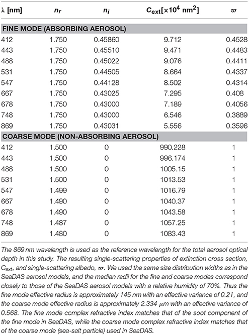
Table 1. The aerosol complex refractive index at the 9 MODIS VIS channels used in this study is based on the SeaDAS model (Ahmad et al., 2010 and see also Figure 1), so that the spectral dependence of the complex refractive index is assumed to be true for a given relative humidity, in other words taken as a priori information.

5. Results

A simple study was conducted to explore the advantage of making use of polarization information. To this end a synthetic dataset was created to simulate the top of the atmosphere (TOA) Stokes parameters I and Q for a range of aerosol optical depths (τ_λref), and optical depth fraction f_τa of absorbing fine mode aerosol particles embedded in a background molecular atmosphere. As mentioned above an efficient forward model was created using a RBF-NN and shown to have good accuracy. The neural network coefficients of the RBF-NN were found using Matlab's newrb function in the Neural Network toolbox. An optimal estimation scheme (see section 4) was employed to retrieve τ_λref, fine mode fraction f_τa, and vertical location of the absorbing aerosols. The resulting retrievals are shown in Figures 5–8.

The “Levenberg-Marquardt” (LM) Marquardt (1963) algorithm is somewhat ambiguous in certain respects. Hence, there may be detail-specific implementation differences between different LM algorithms. Overall, however, we expect that if the algorithm is properly implemented and there is enough information content to perform the retrieval, then these details should mainly affect its performance in terms of efficiency, e.g., the number of iterations needed, as opposed to the final answer, which, if the algorithm has converged, should be equal to the Gauss-Newton optimal estimation result. For example, the threshold for calculating when to increase or decrease the step size γ_i, and by how much, as well as the handling of retrieval parameter values that drift “out-of-bounds,” are implementation-dependent.

The first guess x₀ was calculated using Equation (7) in a direct neural network inversion mapping directly from polarized radiances to retrieval parameters as explained in section 3, called the neural network based first guess. Thus, as seen in Figure 4, with our neural network based first guess, we are able to retrieve optical depth, single-scattering albedo, and vertical location using the set of I and Q measurements at nine VIS channels in the optimal estimation. This result in Figure 4 is thus considered to be our best achievable result, and will be used as our benchmark in the remainder of this paper. It should be noted that the prior x_a is always set equal to the full range of the retrieval parameters. The first guess is either the “naive” assumption, taken to be the midpoint of the range of the aerosol retrieval parameters [x₀ = (0.25, 0.5, 2.0)], or else is set equal to the result from the neural network direct mapping, i.e., the neural network based first guess. The a priori covariance matrix S_a is assumed to be a (Rodgers, 2000) diagonal matrix that is a function of the a priori vector x_a:

$\begin{array}{ll}{S}_a={(10x_a)}^{2}I.& (11)\end{array}$

FIGURE 4

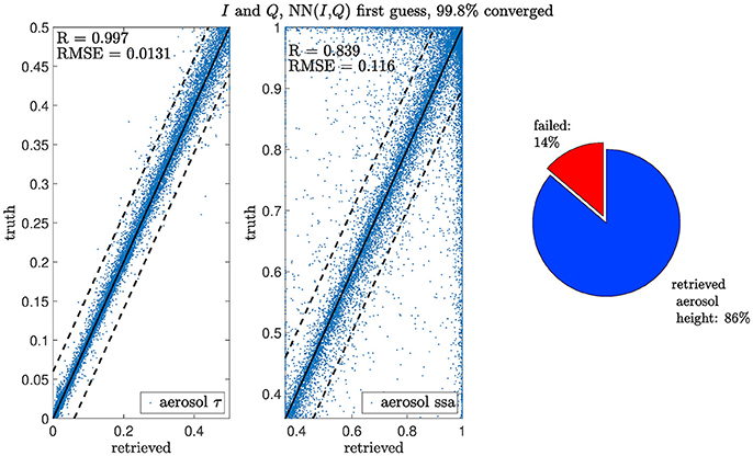
Figure 4. Benchmark retrieval: A synthetic optimal estimation based retrieval of aerosol optical depth at 869 nm and the fraction of absorbing aerosols for MODIS assuming the instrument could measure the Q Stokes parameter in addition to I in nine VIS channels. This retrieval uses the I and Q measurements, and a neural network based first guess using direct inversion. This retrieval is used as a best-case scenario and is considered the benchmark for the other scenarios.

Thus, the covariance matrix of a priori values, S_a, has an assumed variance of ${(10x_a)}^2$ with all non-diagonal elements set equal to 0. These large variance values imply that we are placing little emphasis on the a priori component, since we want to investigate the information contained in the measurements of the system itself.

Figure 5 is based on using both I and Q in the optimal estimation retrieval, as in Figure 4, but not using the neural network based first guess. Instead the first guess was our “naive” assumption, so that x₀ = (0.25, 0.5, 2.0). The retrieval result for this case is seen to be quite good compared to the benchmark. We were able to retrieve both the aerosol optical depth and the fraction, and, in most cases, also the vertical location. This result suggests that either the neural network based first guess is not providing any additional information, and/or there is enough information provided by the set of I and Q measurements to successfully retrieve the three aerosol parameters.

FIGURE 5

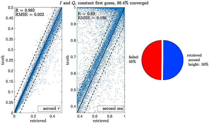
Figure 5. Same as Figure 4 except with a “naive” first guess. A retrieval that makes use of both I and Q, despite using a “naive” first guess, nonetheless appears to work reasonably well for retrieving optical depth and single-scattering albedo, but not aerosol vertical location.

Figure 6 shows how a total radiance-only inversion would perform in the absence of a neural network based first guess, by instead using our “naive” first guess. In contrast with Figure 5, which also was based on the use of a “naive” first guess, we note that the additional information provided by the Q Stokes parameter is very helpful when the first guess is inferior. A comparison of Figure 6 with Figure 7, which compares favorably with the benchmark, shows that an accurate first guess is of crucial importance if the retrieval is based solely on the total radiance.

FIGURE 6

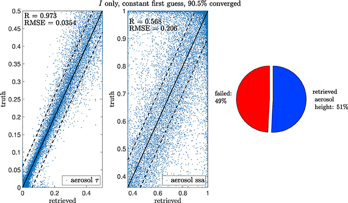
Figure 6. Total radiance-only retrieval except with an “naive” first guess. Identical to Figure 5 except only I was used in the retrieval, not Q. Identical to Figure 7 except a “naive” first guess was used. The total radiance-only retrieval is able to retrieve aerosol optical depth fairly reliably, but not aerosol single-scattering albedo or vertical location.

FIGURE 7

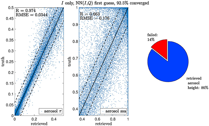
Figure 7. Total radiance-only retrieval. Identical to Figure 4 except only I was used in the retrieval, not Q. By using the neural network based first guess, we are able to retrieve aerosol optical depth and also vertical location when using total radiance-only in the OE/LM retrieval step, but the aerosol single-scattering albedo is more difficult to retrieve.

Figure 7 is also based on using only the total radiance I in the OE/LM optimization scheme. However, the neural network based first guess obtained by use of measurements of both I and Q was employed. The good results obtained from an optimal estimation based solely on I may be surprising, but it is quite reasonable that a starting point close to the solution will help a system converge. Hence, as long as the first guess provides a good estimate, or there is sufficient a priori information, the radiance-only retrieval is expected to work reasonably well for this system. This result also suggests that the direct inversion provided by our neural network based first guess is providing actual information about the system. A comparison of the two retrievals that both use the “naive” first guess, Figures 5, 7, demonstrates that the I, Q set contains enough information to significantly improve retrievals of aerosol single-scattering, without depending on a good first guess or a priori information (beyond the assumed aerosol model that is used), implying that the additional information in the measurements leads to fewer possible solutions. However, retrieval of aerosol vertical location is poor when using the “naive” first guess, suggesting that it may cause a bias, or that our optimal estimation scheme is not completely optimized. However, perfect optimization of the estimation algorithm is beyond the scope of this study, as it is mainly for demonstration purposes, and there are certainly improvements that could be made. The improvement based on the first guess provided by direct inversion using a neural network strongly suggests that the information about aerosol location is also captured by the measurements.

Finally, a summary of the results is provided in Figure 8 which shows that addition of the Q Stokes parameter is required to obtain reliable retrievals of aerosol optical depth, single-scattering albedo (calculated from the aerosol optical depth and fine mode fraction using Equation 5), and vertical location. Success was defined as being within ± 0.03 for the total aerosol optical depth at 869 nm, within ± 0.04 for single-scattering albedo (ssa) at 869 nm and either as correct or incorrect for the aerosol vertical location. The use of I and Q with a NN-based first guess based on I and Q enables retrieval of all three of these parameters 65% of the time, whereas the total radiance-only retrieval can only achieve this accuracy in about 37% of the cases with the same NN-based first guess. As seen in Figures 6, 7, the total optical depth is generally retrievable if only the total radiance is available (79% successful), although that performance is improved to 96% for I and Q with the NN-based first guess. However, the retrieval of the single-scattering albedo is significantly improved with polarization information: 74% of cases are retrieved within ± 0.04 with I and Q and the NN-based first guess, compared to 45% using total radiance-only and the same first guess. We can see that the optimal estimation scheme is likely either not completely optimized, or is being biased by the naive first guess, since there is a large discrepancy between the performance using I and Q measurements with and without the neural network first guess. However, the results show that the retrieval of absorbing aerosol parameters using I and Q measurements is significantly better than that using I measurements alone.

FIGURE 8

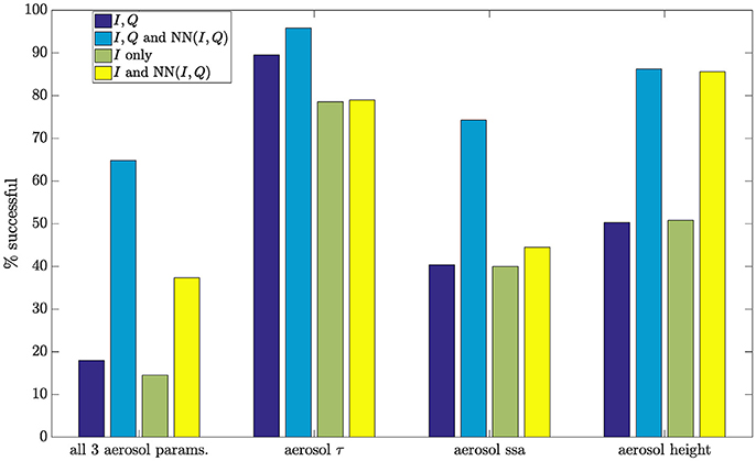
Figure 8. The percentage of success for each of the four retrieval schemes is summarized for each retrieval parameter. Success is defined as being within ± 0.03 for the total aerosol optical depth at 869 nm, within ± 0.04 for single-scattering albedo (ssa) at 869 nm and either as correct or incorrect for the aerosol vertical location. The retrieval using I and Q with a NN-based first guess using I and Q is able to retrieve all 3 of these parameters 65% of the time, whereas the total radiance-only retrieval can only achieve this accuracy in about 37% of cases. As seen in Figures 6, 7, the total optical depth is generally retrievable if only the total radiance is available (79% successful), although that is improved to 96% successful for I and Q with the NN-based first guess. However, the retrieval of the single-scattering albedo is significantly improved with polarization information: 74% of cases are retrieved within ± 0.03 with I and Q and the NN-based first guess, compared to 45% using total radiance-only and the same first guess.

6. Conclusions

In this study, we have explored the feasibility of retrieving accurate values of aerosol optical depth, the fine mode fraction and hence single-scattering albedo, and the vertical location of absorbing aerosol particles from measurements of the I and Q components of the Stokes vector. We have found that use of total radiance-only (the I component) is generally insufficient to retrieve accurate values of these three retrieval parameters. It appears, however, that use of an accurate first guess based on a neural network direct inversion using both I and Q, provides significant improvement. Based on this accurate first guess, retrievals based on total radiance-only yield good results. Hence, use of accurate forward model simulations of the polarized radiation could improve retrievals based on existing optimal estimation schemes, which employ total radiance-only measurements. In fact, little modification to the existing schemes would be required, since only the neural network derived first guess (using both I and Q measurements) would need to be added. However, use of Q and I in combination leads to significantly improved retrievals of aerosol fine mode fraction (and thus single-scattering albedo), and vertical location in the case of the neural network derived first guess, and can also retrieve all three aerosol parameters with the “naive” first guess, corresponding to little a priori knowledge of the system. The improvement resulting from the use of a neural network based first guess, and the OE/LM retrieval with both I and Q, implies that there is significant information contained in the set of I and Q measurement pairs, and that the remote sensing capability of spectroradiometers (like MODIS and MERIS) could be significantly enhanced by measuring Q in addition to I. This proof-of-concept algorithm demonstrates that it is possible to use neural networks not only for the first guess, but also for the forward model that generates TOA total and polarized radiances, which can enable operational processing of high-density imaging data from moderate and hyperspectral resolution imaging sensors measuring total and polarized radiances using optimal estimation.

7. Future Work

Future work would involve quantifying the amount of information content added by the Q Stokes parameter including for ocean-color retrieval parameters, and whether it is possible to discriminate between two fine mode mixtures of absorbing and non-absorbing aerosols. It would also be interesting to explore the use of more sophisticated and powerful multi-layer neural networks for the direct inference of the retrieval parameters (Fan et al., 2017). This proof-of-concept algorithm could also be applied to real data, although work would be needed to identify the proper set of aerosol models based on available a priori information, since some assumptions about the aerosol models may still be required (e.g., for total radiance measurements made from a single angle, parameterizing the median radius and spectral complex refractive index as a function of relative humidity, like in the SeaDAS aerosol models, although depending on the channels used perhaps the relative humidity parameter could also be retrieved). In addition to exploring the added aerosol information provided by the U Stokes parameter, we note that multi-angular and/or hyperspectral measurements would also provide additional information about each pixel, the processing of which would also greatly benefits from fast methods of computing the TOA total and polarized radiance. Lastly, although we used a fixed random Gaussian measurement noise profile with a standard deviation of 3% for both Stokes parameters, the accuracy of retrieved aerosol/ocean products could be analyzed as a function of instrument performance.

Author Contributions

All authors listed, have made substantial, direct and intellectual contribution to the work, and approved it for publication.

Funding

The work described in this paper was partially funded by the NASA Aerosols-Clouds-Ecosystems (ACE) mission and by the Japanese Aerospace Exploration Agency (JAXA) through a grant to Stevens Institute of Technology.

Conflict of Interest Statement

The authors declare that the research was conducted in the absence of any commercial or financial relationships that could be construed as a potential conflict of interest.

References

Ahmad, Z., Franz, B. A., McClain, C. R., Kwiatkowska, E. J., Werdell, J., Shettle, E. P., et al. (2010). New aerosol models for the retrieval of aerosol optical thickness and normalized water-leaving radiances from the SeaWiFS and MODIS sensors over coastal regions and open oceans. Appl. Opt. 49, 5545–5560. doi: 10.1364/AO.49.005545

PubMed Abstract | CrossRef Full Text | Google Scholar

Broomhead, D. S., and Lowe, D. (1988). Radial Basis Functions, Multi-variable Functional Interpolation and Adaptive Networks. Technical Report, DTIC Document.

Cohen, D., Stamnes, S., Tanikawa, T., Sommersten, E. R., Stamnes, J. J., Lotsberg, J. K., et al. (2013). Comparison of discrete ordinate and monte carlo simulations of polarized radiative transfer in two coupled slabs with different refractive indices. Opt. Exp. 21, 9592–9614. doi: 10.1364/OE.21.009592

PubMed Abstract | CrossRef Full Text | Google Scholar

Di Noia, A., Hasekamp, O. P., Wu, L., van Diedenhoven, B., Cairns, B., and Yorks, J. E. (2017). Combined neural network/Phillips–Tikhonov approach to aerosol retrievals over land from the nasa research scanning polarimeter. Atmosph. Meas. Tech. 10:4235. doi: 10.5194/amt-10-4235-2017

CrossRef Full Text | Google Scholar

Fan, L., Li, W., Dahlback, A., Stamnes, J. J., Stamnes, S., and Stamnes, K. (2014). New neural-network-based method to infer total ozone column amounts and cloud effects from multi-channel, moderate bandwidth filter instruments. Opt. Exp. 22, 19595–19609. doi: 10.1364/OE.22.019595

PubMed Abstract | CrossRef Full Text | Google Scholar

Fan, Y., Li, W., Gatebe, C. K., Jamet, C., Zibordi, G., Schroeder, T., et al. (2017). Atmospheric correction over coastal waters using multilayer neural networks. Remote Sens. Environ. 199, 218–240. doi: 10.1016/j.rse.2017.07.016

CrossRef Full Text | Google Scholar

Gordon, H. R. (1997). Atmospheric correction of ocean color imagery in the earth observation system era. J. Geophys. Res. 102, 17081–17106. doi: 10.1029/96JD02443

CrossRef Full Text | Google Scholar

Gordon, H. R., and Wang, M. (1994). Retrieval of water-leaving radiance and aerosol optical thickness over the oceans with sea-wifs: a preliminary algorithm. Appl. Opt. 33, 443–445. doi: 10.1364/AO.33.000443

CrossRef Full Text | Google Scholar

Hasekamp, O. P., Litvinov, P., and Butz, A. (2011). Aerosol properties over the ocean from parasol multiangle photopolarimetric measurements. J. Geophys. Res. Atmosph. 116:D14204. doi: 10.1029/2010JD015469

CrossRef Full Text | Google Scholar

Herman, M., Deuzé, J.-L., Marchand, A., Roger, B., and Lallart, P. (2005). Aerosol remote sensing from polder/adeos over the ocean: improved retrieval using a nonspherical particle model. J. Geophys. Res. Atmosph. 110:D10S02. doi: 10.1029/2004JD004798

CrossRef Full Text | Google Scholar

Imaoka, K., Kachi, M., Fujii, H., Murakami, H., Hori, M., Ono, A., et al. (2010). Global change observation mission (gcom) for monitoring carbon, water cycles, and climate change. Proc. IEEE 98, 717–734. doi: 10.1109/JPROC.2009.2036869

CrossRef Full Text | Google Scholar

Leroy, M., and Lifermann, A. (2000). The polder instrument onboard adeos: scientific expectations and first results. Adv. Space Res. 25, 947–952. doi: 10.1016/S0273-1177(99)00927-8

CrossRef Full Text | Google Scholar

Li, W., Stamnes, K., Spurr, R., and Stamnes, J. (2008). Simultaneous retrieval of aerosol and ocean properties by optimal estimation: seawifs case studies for the santa barbara channel. Int. J. Remote Sens. 29, 5689–5698. doi: 10.1080/01431160802007632

CrossRef Full Text | Google Scholar

Marquardt, D. W. (1963). An algorithm for least-squares estimation of nonlinear parameters. J. Soc. Indust. Appl. Math. 11, 431–441. doi: 10.1137/0111030

CrossRef Full Text | Google Scholar

Rodgers, C. (2000). Inverse Methods for Atmospheric Sounding. Singapore: World Scientific.

Google Scholar

Shettle, E. P., and Fenn, R. W. (1979). Models for the Aerosols of the Lower Atmosphere and the Effects of Humidity Variations on Their Optical Properties. Technical report, DTIC Document.

Spurr, R., Stamnes, K., Eide, H., Li, W., Zhang, K., and Stamnes, J. (2007). Simultaneous retrieval of aerosols and ocean properties: a classic inverse modeling approach. I. Analytic jacobians from the linearized cao-disort model. J. Quant. Spectr. Radiat. Transf. 104, 428–449. doi: 10.1016/j.jqsrt.2006.09.009

CrossRef Full Text | Google Scholar

Stamnes, K., Li, W., Eide, H., and Stamnes, J. J. (2005). Challenges in atmospheric correction of satellite imagery. Opt. Eng. 44:041003–1–041003–9. doi: 10.1117/1.1885469

CrossRef Full Text | Google Scholar

Stamnes, K., and Stamnes, J. J. (2015). Radiative Transfer in Coupled Environmental Systems. Weinheim: Wiley-VCH.

Google Scholar

Stamnes, K., Thomas, G. E., and Stamnes, J. J. (2017). Radiative Transfer in the Atmosphere and Ocean, 2nd Edn. Cambridge, UK: Cambridge University Press.

Tanikawa, T., Li, W., Kuchiki, K., Aoki, T., Hori, M., and Stamnes, K. (2015). Retrieval of snow physical parameters by neural networks and optimal estimation: case study for ground-based spectral radiometer system. Opt. Exp. 23, A1442–A1462. doi: 10.1364/OE.23.0A1442

PubMed Abstract | CrossRef Full Text | Google Scholar