Sensitivity of Convection-Permitting Regional Climate Simulations to Changes in Land Cover Input Data: Role of Land Surface Characteristics for Temperature and Climate Extremes

Introduction

Efficient emission reduction policies are needed to reduce the rate of climate change intensification with increasing greenhouse gas emissions. This reduction requires development of mitigation and adaptation strategies for the sustainable use of resources, where land-atmosphere interactions are considerably important (Betts 2007; de Noblet-Ducoudré and Pitman, 2021). According to the IPCC (2013), a key role is played by land transformations in adapting and mitigating climate change for future scenarios with the aim to stabilize temperature increases up to 1.5°C. Land use/cover change influences the regional and local climate due to its interaction with the atmosphere via biogeophysical and biogeochemical processes. In recent decades, many modeling groups have revealed the importance of the land surface in numerical models over various temporal and spatial scales (Sellers et al., 1996; Brovkin et al., 2004). These findings resulted in the inclusion of land use/cover forcings in the climate projections of the Coupled Model Intercomparison Project Phase 5 (CMIP5, Hurtt et al., 2011). The results revealed that the land surface forcing can be as high as the forcing due to the RCP2.6 scenario based on global circulation models (de Noblet- Ducoudré et al., 2012). A first-of-its-kind future land cover change study based on a single convection-permitting regional climate model concluded that increased cultivation of bioenergy crops by poplar trees can reduce future local maximum temperatures by up to 2°C in mid Europe (Tölle et al., 2014).

Land surface characteristics depending on the soil, vegetation, urban area, and topography play an important role in influencing climatic patterns or meteorological events. For example, synoptic systems can be blocked by topography (Barrett et al., 2015), or precipitation patterns can be influenced by soil moisture—precipitation feedbacks (Hohenegger et al., 2009; Seneviratne et al., 2010; Wei and Dirmeyer 2012). Through their albedo and evapotranspiration capabilities and aerodynamic roughness, vegetation and urban areas can affect temperature variations and the boundary layer height (Tölle et al., 2017; Tölle et al., 2018; Belušić et al., 2019; Davin et al., 2020; Hertwig et al., 2020). Accounting for biogeochemical fluxes between the land surface and the atmosphere is considered to be as important as biogeophysical fluxes in representing the biomass evolution of vegetation including carbon, water and nutrients. Each of the land surface characteristics influences soil moisture and the partitioning between the energy and water fluxes of different strengths with spatiotemporal heterogeneity (McCabe and Wolock 2013). The atmosphere responds through changes in temperature and humidity, precipitation and cloud cover. Circulation patterns can even be changed (Zhao et al., 2001) depending on the magnitude of land transformation. Soil moisture heterogeneities arise from these processes (McCabe and Wolock 2013). Thus, to realistically simulate land use/cover change effects on regional and local climate and draw conclusions for management strategies, numerical models would benefit from land surface characteristics, which are as accurate as possible and have high spatial resolution. Furthermore, the numerical models require a high spatial resolution in terms of their grid sizes to simulate such feedbacks.

Convection-permitting models (Prein et al., 2015) enable representation of the land surface below 4 km and improve regional forcing and processes (Garnaud et al., 2015). Changes in local conditions with the underlying surface including heat and water storage capacities have the largest impact on temperature due to the interplay between surface albedo and evapotranspiration efficiencies (Tölle et al., 2014). Thus, significant changes in the temperature response are expected locally, underpinning the importance of the convection-permitting scale when considering land use/cover changes.

The lower boundary of a climate model is a soil vegetation atmosphere transfer scheme (SVAT) for exchanging heat, moisture, and momentum with the atmosphere. These schemes require several parameters that describe the land surface, including orography, land-water masks, soil and vegetation characteristics or urbanized area locations as input data, which are derived from remote sensing observations or in situ measurements. Commonly used surface parameters for vegetation parameterization are the leaf area index and the minimal or maximal stomatal resistance, which are important for transpiration processes through the leaves, and the vegetation fraction, which determines the amount of evapotranspiration from the surface. The wind, humidity and temperature profiles between the surface and lower atmosphere are influenced by the roughness length, which plays a role in turbulent exchange processes with the atmosphere. The surface albedo and emissivity determine the energy availability at the surface. The root depth determines the water extracted from the soil layers by plants.

Presently, several land cover maps are available for regional climate and weather models such as the products based on MODIS (Friedl et al., 2010), GLC 2000 (Bartholomé and Belward 2005), GlobCover 2009 (Arino et al., 2008), and CCI (Poulter et al., 2015; Li et al., 2018). The land cover of these products is static in time for the regional climate simulations. The impact of time-varying land cover data in regional climate models is currently investigated in a joined community effort, which is the Land Use and Climate Across Scales Flagship Pilot Study (LUCAS FPS) supported by the World Climate Research Program-Coordinated Regional Climate Downscaling Experiment (WCRP-CORDEX) and was initiated by the European branch of CORDEX (EURO-CORDEX) (Davin et al., 2020). The land cover data have a global distribution and are retrieved from satellite observations. They define the boundaries between ecosystems, such as forests, wetlands, and cultivated systems.

The GlobCover2009 land cover map was developed by the European Space Agency (ESA) with the assistance of ENVISAT’s Medium Resolution Imaging Spectrometer (MERIS) instrument at 300 m resolution (Arino et al., 2008). This 2009 land cover map is available within a year of the last satellite acquisition. The legend of the map, including 22 different land cover classes, is related to the UN Land Cover Classification System (LCCS, Di Gregorio and Jansen 2000). Its predecessor GLC 2000 (Global Land Cover map for the year 2000, Bartholomé and Belward 2005) is the result of a coordinated project by the European Commission’s Joint Research Centre (JRC) and ESA. The data product provides a harmonized land cover database for the year 2000 on a 1 km spatial resolution. The 22 land cover types are based on an older (FAO 1988) LCCS with a slight different classification than that of GlobCover 2009. Daily data are retrieved from the VEGETATION sensor onboard SPOT 4 satellite. The ESA developed another data product, the Climate Change Initiative with Land Cover (CCI_LC), at 300 m resolution based on time-varying land cover data (Bontemps et al., 2012; Poulter et al., 2015). Data are retrieved from the MERIS and VEGETATION 1 and 2 instruments onboard ENVISAT and SPOT 4 and 5. The dataset can be obtained with 22 or 38 standard thematic classes or a user-defined setup with cross-walking tables. The classification is based on UN LCCS. The land cover data are available from 1992 to 2015. ECOCLIMAP (Masson et al., 2003; Champeaux et al., 2005) is a global database with 243 land cover classes at 1 km resolution based on NOAA/AVHRR satellite data (Champeaux et al., 2000) and developed in collaboration with the University of Maryland (Hansen et al., 2000; Loveland et al., 2000). The procedure for Europe differs to some extent. Here, the land cover classes are derived from the Coordination of Information on the Environment (CORINE) land cover database (CEC 1993; Heymann, 1993), which has a 250 m spatial resolution and then averaged to 1 km. Data gaps in the CORINE database are filled with Pan-European Land cover Monitoring (PELCOM) data (Mucher et al., 2001).

The land cover classes are combined with climate maps of the world (Kottek et al., 2006), such as the KÖPPEN-GEIGER climate classification map to retrieve a discrimination among ecosystems on each continent. Typical climates of Köppen climate zones are: Af (equatorial rainforest and full humid), Am (equatorial monsoon), Aw (equatorial savannah), BW (desert climate), BS (steppe climate), Cs (warm temperate climate with dry summer), Cw (warm temperate climate with dry winter), Cf (warm temperate climate and fully humid), Ds (snow climate with dry summer), Dw (snow climate with dry winter), Df (snow climate and fully humid), ET (tundra climate), and EF (frost climate). The vegetation parameters for the numerical models are ultimately derived from these ecosystems.

Spatial inconsistencies exist among global land cover datasets (Hua et al., 2018). This uncertainty accumulates in the whole processing chain of remote-sensing information by obtaining, processing, analyzing and expressing the results. Thus, the land cover maps differ in land cover classes and their numbers, class fraction and spatial distribution, spatial resolution, and year of retrieval. Using one land cover map over the other in a climate or weather model eventually leads to differences in vegetation parameters or urban area distribution affecting the regional and local climate. For example, Heret et al. (2006) report changes in the latent heat flux of 90% when the LAI is changed from 1 to 5. The importance of land cover uncertainties on climate compared to climate projection uncertainties is of current debate. This stresses the need to quantify the sensitivity of models results to changes in land cover input data.

Therefore, this study investigates the uncertainty in regional climate modeling by analysing the impact of different land cover maps in the official regional climate model Consortium of Small-scale Modeling (COSMO)-CLM (CCLM, Rockel et al., 2008) on regional and local climate. The research questions, which we address, are:

1. What is the impact on regional and local climate due to changes in retrieval year, number, fraction and spatial distribution of land cover classes?

2. What is the role of the surface parameters on the surface turbulent fluxes and temperature?

3. How do land cover class spatial distribution changes between the surface maps effect seasonal climate extremes?

Note that the official version of CCLM treats urban surfaces as a land cover class without anthropogenic heat flux or urban albedo (Trusilova et al., 2016). Non-hydrostatic convection-permitting climate simulations are performed at 3 km spatial resolution over Germany from 2002 to 2011. Simulations are directly downscaled (Coppola et al., 2018; Ban et al., 2021) with ERA5 reanalysis data (Hersbach et al., 2018). If the retrieval year varies in the same dataset, as in the CCI data, changes in land cover class fraction and spatial distribution can be regarded as a land cover change. However, differences in retrieval year among the land cover maps do not necessarily reflect land cover change. The resulting spatial discrepancies can also be due to differences in data processing. There is an increase in quality of information between older and new land cover products with respect to the representation of urbanized areas (Katzfey et al., 2020). The former land cover of the CCLM was based on GLC200. At present, the CCLM uses the land cover map GlobCover 2009, which is also the dataset for operational weather forecasts with COSMO or most recently ICON. If the CCI provides advantages over GlobCover2009 in the CCLM needs to be determined. In addition, an analysis is beneficial for providing suggestions for use in land use/cover change and management studies with regional climate models for climate adaptation strategies. This study is the first in the literature on the long-term impact of different land cover datasets on climate at convection-permitting scale.

The following section describes the methodology, including the study area, a description of CCLM, simulation experiments, datasets used and statistical methods. The results are presented in section Results. In section Discussion and Conclusion the results are discussed and conclusions are drawn.

Methodology

Regional Climate Model and Set-Up

The region of the simulation domain covers Germany with adjacent areas as shown in Figure 1. The CCLM (v5.0_clm16) used for simulations with different land cover maps is based on the COSMO, which is a limited-area model designed for applications at the meso-β to meso-γ scales (Baldauf et al., 2011). A one way nesting with Davies-type lateral boundary formulation is applied at the lateral boundaries. A Rayleigh damping layer is used at the top of the model domain. The selection of different dynamical and physical parameterization schemes allows for application of the model at a wide range of spatial and temporal scales from 1 to 50 km. The model integrates the fully compressible, non-hydrostatic thermodynamic equations in a moist atmosphere. The equations are solved numerically on an Arakawa-C staggered grid (Arakawa and Lamb 1977) in rotated coordinates, with a Runge-Kutta time-stepping scheme (Wicker and Skamarock 2002). The model uses a vertical terrain-following height coordinate (Doms and Baldauf, 2013). A one-moment microphysics scheme, including five categories of hydrometeors (clouds, rain, snow, ice, and graupel), is used for the parameterization of precipitation. The simulations use a modified Tiedtke parameterization of shallow convection. Deep convection is resolved, enabling determination of the resolution of convective processes. The radiative transfer scheme is based on Ritter and Geleyn (1992), and a turbulent kinetic energy-based surface transfer and planetary boundary layer parameterization (Raschendorfer 2001) is applied. Here, a stability and roughness length dependent surface flux formulation couples the atmosphere with the underlying surface based on drag-law formulations (Doms et al., 2013). The surface flux of sensible heat/water vapour depend beside the bulk-aerodynamical transfer coefficient on the gradient between the prognostic temperature/specific humidity at the lowest grid level above the ground and surface temperature/ground level specific humidity.

FIGURE 1

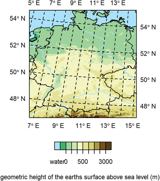
FIGURE 1. Geometric height in meters of the Earth’s surface above sea level for the simulation domain.

The soil-vegetation-atmosphere transfer (SVAT) module TERRA-ML (Schrodin and Heise 2002; Doms et al., 2013) provides the surface temperature and specific humidity at the ground for calculating the surface fluxes as lower boundary for the atmospheric part of the model. The ground temperature is calculated by the equation of heat conduction. There are 10 active layers with a depth of 15.34 m for energy calculations. The soil water content is predicted by the Richards equations. Eight active layers with depth of 3.82 m are assumed for water transport calculations. Evaporation from bare soil and transpiration by plants adopted from Dickinson (1984) are functions of the water content. Transpiration is additionally determined by radiation and ambient temperature.

The land surface parameters (soil type, plant characteristics, orography, etc.) are processed with the external parameter tool EXTPAR (Smiatek et al., 2008) to align with the model’s spatial resolution. The vegetation characteristics are hereby calculated from the dominant land cover by application of look-up tables (Doms et al., 2013). The external parameters contain orography and coastlines based on ASTER (Advanced Space borne Thermal Emission and Reflection Radiometer) data (NASA 2019), which is valid for the region between 60°S and 60°N. The soil type and depth data were adapted from the Harmonized World Soil Database (HWSD, Fischer et al., 2008). Nine soil types are considered and refer to the upper 30 cm of the dominant soil. The temperature climatology of the lowest soil layer is based on the Climate Research Unit (CRU) data at 0.5° spatial resolution from the University of East Anglia (New et al., 1999). The aerosol climatology comes from the National Aeronautics and Space Administration Goddard Institute for Space Studies (NASA GISS, Tegen et al., 1997). The surface albedo climatology is determined from TERRA MODIS (Schaaf and Wang 2015). This albedo is prescribed by external fields and defined in EXTPAR. Average values for every month are provided. The actual surface albedo is determined by a linear interpolation between two monthly values, depending on the day. The energy is then partitioned depending on the surface/vegetation parameters influencing the surface fluxes. The latent heat flux (LE) depends on the vegetation cover fraction and leaf area index. The sensible heat flux (SH) is also related to vegetation through its partition with the latent heat flux and the aerodynamic exchange specific to the surface/vegetation type.

Each land cover class has corresponding surface parameters, which are prescribed as look-up tables in the model (Doms et al., 2013). The surface parameters for each land cover class include vegetation cover fraction (PLCOV), leaf area index (LAI) and rooting depth (RD). A sinusoidal fit between the maximum and minimum LAI according to the Julian day, elevation and latitude results in seasonality (Doms et al., 2013) with a static annual cylce. The LAI seasonality can also be imposed by monthly values of the normalized difference vegetation index (NDVI) derived from the AVHRR visible and near-infrared spectral bands, assuming a proportionality between the NDVI and LAI. The vegetation cover fraction and roughness length (Z0) are analytically calculated from the LAI and land cover class. The roughness length depends on land cover and subgrid-scale orography. Urban areas in the official version of the RCM are treated as a land cover class with associated surface parameters. Thus, the urban impervious surfaces are presented as natural land surfaces with increased surface roughness (Z0 = 1.0) and reduced vegetation cover (maximum PLCOV = 0.2). No anthropogenic heat flux, urban canopy layer or urban surface energy balance are included in the simulations (see Trusilova et al., 2016).

Simulation Experiments and Data Analysis

The simulations were run with 50 atmospheric layers, a model top of 22 km, and a time step of 25 s each. The configuration was adapted from the COSMO-DE setup of the German Weather Service with modifications based on several sensitivity test runs. Simulations were conducted as direct downscaling experiments at convection-permitting scale driven by ERA5 reanalysis data (Hersbach et al., 2018) with a horizontal resolution of approximately 3 km over the whole of Germany. The horizontal extent of the simulation domain is smaller by 2 grid boxes at each side than the total model domain. This sponge zone allows to implement the boundary conditions and to apply the domain decomposition strategy. The whole model domain is initialized with the meteorological variables (specific humidity, air temperature, surface pressure, wind components, specific cloud liquid water and ice content, etc.) from the driving data as and the lateral boundary conditions are updated for each time step thereafter. The soil temperature and moisture profiles are initialized at the start of the simulation for the whole simulation domain and updated afterwards at the lateral boundaries.

The simulations were conducted with four different land cover maps, namely GlobCover 2009 (GC), GLC 2000 (GLC), ECOCLIMAP (ECO), and CCI. Table 1 lists all of the simulation experiments conducted with the land cover maps used, the retrieval year, the land cover classes and the reference source of the data. The CCI land cover map is retrieved for 2000 (CCI) and 2015 (CCI 2015) to examine the impact of land cover change over time. For 2015, two simulations based on the CCI had different numbers of land cover classes. One simulation contains 22 land cover classes, and the other simulation has 38 land cover types (named CCI38 in the following). ECO contains 243 land cover classes. This difference allows to study the changes due different number of land cover classes. GLC, CCI, and CCI2015 share the same land cover types (Zhang, Tölle et al., 2021). GC shares the same number of land cover classes, which are comparable to the ones of GCL. Difference thus arise from land cover class fraction and spatial distribution.

TABLE 1

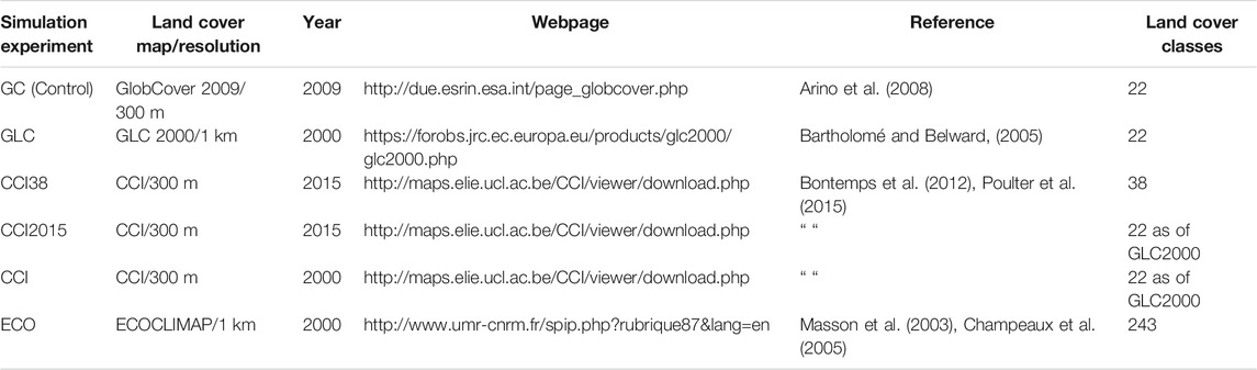
TABLE 1. Names of simulation experiments including the land cover map used and spatial resolution, the retrieval year of the land cover maps, their sources and references with the respective numbers of land cover classes. The simulation experiment GC, which uses the land cover map GlobCover 2009, is the reference or control simulation to which the other simulation experiments are compared.

The simulation with the GC land cover map is used as the reference simulation to which the other simulations are compared to. GC is the current operational land cover dataset of the German Meteorological Service. The simulation with GC is conducted from 2000 to 2011, where the first year 2000 is discarded from the analysis of a spin-up year. The other simulations started in 2001 with balanced soil moisture conditions. Finally, the analysis for all simulations is over a 10-years period from 2002 to 2011. All the simulations have the same lateral boundary conditions, and the experimental simulations started with balanced soil moisture conditions from the reference simulation. The simulated circulation is similar for the simulations due to the small domain and ERA5 forcing at the boundaries. Thus, changes can be attributed to the differences in land cover maps.

The land cover maps described in Table 1 have different land cover legends with different land cover classes. A detailed list of the land cover classes of the maps is provided in the supplementary material. For example, typical classes include evergreen needleleaf forest, evergreen broadleaf forest, deciduous needleleaf forest, deciduous broadleaf forest, mixed forest, woodland, grassland, closed and open shrubland, cropland, wetlands, bare soil, urban areas, water, permanent snow and ice. GC includes mixed versions of these classes with different fractions. Thus a harmonization for comparison analysis is required. For example, GC uses the UN LCCS classification scheme with 22 classes, whereas ECO is based on another classification system that is supported by the EU commission and has 243 classes. To compare the differences in fraction and spatial distribution among the land cover classes of the maps, the land cover fractions are aggregated and normalized to form a set of unified and generalized classes. The six new resampled consistent land cover groups correspond to natural vegetation, crops, pasture, bare soil, urban area, and water. Shrubs and trees are both merged into natural vegetation, and pasture includes grasses. These six land cover types are commonly used in vegetation models, such as CARbon Assimilation In the Biosphere (CARAIB; Warnant et al., 1994). The data and results were examined individually prior to aggregation, which led to the harmonization concept to summarize the results. Then, the differences in local and regional climate due to differences in the six land cover groups between simulations are analyzed.

To evaluate the climate impact due to the different land cover maps, we analyze the temperature, latent and sensible heat fluxes and vegetation parameters of the simulation experiments in a coherent way. Cities are presented as a land cover class. As such, urban areas are included by this examination. The analysis is based on the anomalies of the aforementioned variables of the simulation experiments with respect to the reference simulation climatology. The difference corresponds to the experimental simulation minus the control/reference simulation. Temperature and its minimum and maximum value are examined as it is the most affected variable due to changes in the vegetation parameters in the model. The physical processes of the surface energy balance affect this variable. Differences in vegetation parameters result from discrepancies in the land cover classes of the land cover maps. The main vegetation parameters in the model, that influence evapotranspiration, are the LAI, PLCOV and Z0. The LAI is one of the most important parameters since it determines plant transpiration. The LAI is defined as the surface area of leaves contained in a vertical column normalized by its cross-sectional area. Another parameter in this context is PLCOV, which is the fractional area of the grid cell covered by plants. PLCOV estimates the fraction of evapotranspiration by plants. Z0 determines the turbulent exchange of water and heat between the surface and the atmosphere. The latent heat flux depends on these parameters, which may influence the temperature due to its magnitude of evaporative cooling. Therefore, the whole process chain of the differences with respect to the control simulation is examined. We analyse the seasonal variations based on the annual cycle and regionalism based on the parameter distribution over the simulation domain and apply linear regression analysis. In particular, we look at changes in surface parameters [Δ(LAI, PLCOV, Z0)], which may results in differences in the latent heat flux ΔLE. Changes in latent heat flux may be seen in temperature via evaporative cooling [Δ(LAI, PLCOV, Z0) -> ΔLE -> Δ(T2M, Tmax, Tmin)]. Changes in sensible heat flux are additionally analysed.

“Whisker” box plots of monthly climatologies are used for land cover change signal analysis. The central mark in the box plots indicates the median, and the bottom and top edges of the box indicate the 25th and 75th percentiles. Here, differences in daily maximum temperature, daily latent and sensible heat fluxes indices due to land cover changes are examined. The climate indices considered cover growing season length (GSL), growing season start (GSS), ice days (ID), tropical nights (TR), frost days (FD), and number of summer days (SU) listed in Table 2. These indices are important for plant growth, and thus far have not been investigated with land cover change studies in regional climate models at convection-permitting scale. The difference area was calculated for grid cells where a major land cover type change occurred between the control simulation and one of the experimental runs. The land cover type change is dominant if the land cover class fraction changes in a grid box more than 40%. Considered are natural vegetation, pasture and crops changes into urban type in a grid box, or crops and natural vegetation changes into pasture, or pasture change into crops.

TABLE 2

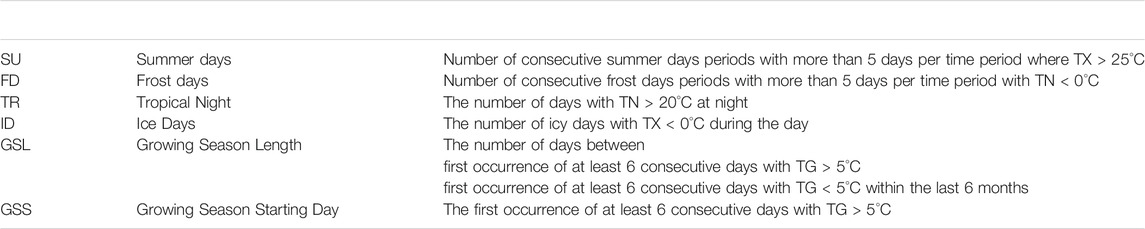
TABLE 2. Subset of the standard ETCCI indices, their abbreviations, and their descriptions. The climate indices are calculated for each experiment described in Table 1. TX is daily maximum temperature, TN is daily minimum temperature and TG is daily mean temperature.

Prior to this analysis the simulation experiments are compared with observations. The HYRAS high-resolution observational dataset from the German Weather Service (Razafimaharo et al., 2020) is used to evaluate the simulation results. These data are gridded daily at 5-km horizontal resolution based on station data, which are available over all of Germany for the period of 1951–2015. The 2-m temperature, including its minimum and maximum temperatures, are extracted from this dataset for the analysis period of 2002–2011.

Statistical performance indices are used to estimate the added value of the simulated temperature (T2M, Tmax and Tmin) with different land cover maps (CCI, CCI 2015, CCI38, GLC, and ECO) with respect to the reference map, which is GC, to the HYRAS observations. Daily values are evaluated for the mean bias error (difference of the model minus observations), the root-mean-square error (RMSE), and the Pearson correlation coefficient (ρ). The RMSE and ρ reflect the quality and spatial consistency between the simulations and observations. We applied additional indices, including the Kling-Gupta-Efficiency (KGE) index (Gupta et al., 2009) and the distribution added value (DAV) index (Soares et al., 2017). The KGE is traditionally used as a goodness-of-fit measure for runoff model performance. Both indices are used by Raffa et al. (2021) to determine the benefit of higher spatial resolution climate simulations compared with coarser spatial resolution climate simulations with respect to observations. We adopted these indices for our study to estimate the benefits of the different land cover maps. The aim of the KGE is to reveal the performance of a model time-series (subscript EXP) with respect to the observational time-series (subscript OBS). KGE equals one demonstrates that there is perfect mapping between the experiment and control data. KGE values lower than −0.41 correspond to underperformance with respect to the mean of the control (observational) data.

$\mathit{KGE}=1-\sqrt{{(\mathit{\rho }-1)}^2+{(\frac{{\mathit{\sigma }}_{\mathit{EXP}}}{{\mathit{\sigma }}_{\mathit{OBS}}}-1)}^2+{(\frac{{\mathit{\mu }}_{\mathit{EXP}}}{{\mathit{\mu }}_{\mathit{OBS}}}-1)}^2}$(1.1)

where ρ is the Pearson correlation coefficient, $\sigma$ is the standard deviation and $\mu$ is the mean value.

The DAV estimates the added value by comparing the probability density function (PDF) of the simulation based on one of the alternative land cover maps and the PDF of the simulation based on the reference land cover map compared with the observational PDF. Moreover, the DAV index allows us to estimate the Perkins skill scores (S) in the experiment based on one of the alternative land cover maps (subscript EXP) and the control simulation based on the reference land cover map (subscript CTR) and the observations (subscript OBS).

$\mathit{DAV}=\frac{{\mathit{S}}_{\mathit{EXP}}-{\mathit{S}}_{\mathit{CTR}}}{{\mathit{S}}_{\mathit{CTR}}}=\frac{{{\displaystyle \sum }}_1^{\mathit{n}} min\left({\mathit{Z}}_{\mathit{EXP}},\mathit{ }{\mathit{Z}}_{\mathit{OBS}}\right)-{{\displaystyle \sum }}_1^{\mathit{n}} min\left({\mathit{Z}}_{\mathit{CTR}}, \mathit{ }{\mathit{Z}}_{\mathit{OBS}}\right)}{{{\displaystyle \sum }}_1^{\mathit{n}} min\left({\mathit{Z}}_{\mathit{CTR}}, \mathit{ }{\mathit{Z}}_{\mathit{OBS}}\right)}$(1.2)

where Z is the frequency of values in each bin for the experiment, reference and observations. In the case, when the DAV equals to zero, there is no benefit due to the alternative land cover map in the climate variable. If the DAV is less than zero, there is a loss in performance due to the alternative land cover map. Positive values of the DAV index demonstrate that there is a beneficial impact due to the alternative land cover map compared with the reference map with respect to the observations.

Results

The six dominant land cover fractions of the simulations with the regional climate model CCLM and the fraction difference with respect to the reference simulation based on GC are presented in Figures 2A,B. The six major land cover types of each simulation are very similar to each other in their fractions. Cropland and natural vegetation were the most common land cover categories in all the simulation experiments. Approximately 35–40% of the grid cells are covered by crops, and ∼30% are covered by natural vegetation. The rest represents other categories: 10–18% is pasture, 2–8% are urban areas, below approximately 1% is bare soil, and the rest is water. The crop area of the simulation based on GLC is approximately 4.8% higher than that of GC, followed by ECO with 2.5%, and is reduced by more than 2% for the simulations based on CCI. The urban fraction of all simulation experiments is higher than the reference simulation, by 1% for GLC and by approximately 3% for the simulations based on the CCI and ECO. The natural vegetation area decreased by approximately 2% in all the experiments. Major decreases of natural vegetation by 7% are shown for ECO. The pasture fraction decreases for GLC (∼2.5%) and increases for the CCI (∼1.5%) and ECO (∼1.9%) compared with GC. Fraction differences among the simulations based on CCI are similar and of small magnitude. Therefore, arrows showing the magnitude difference between the CCI data are added for visibility. CCI38 has the highest urban (increase) and crop (decrease) fraction difference. The urban and pasture areas are slightly higher for CCI2015 than for CCI and slightly lower for natural vegetation and crops.

FIGURE 2

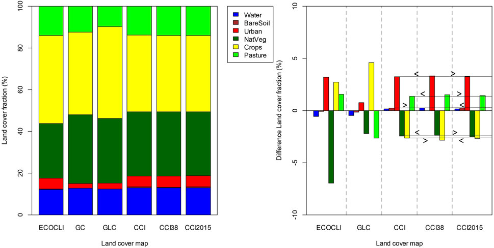
FIGURE 2. (A) Land cover fraction in percent of water (blue), bare soil (brown), urban (red), natural vegetation (green), crops (yellow), and pasture (light green) of each simulation experiment based on ECO, GC, GLC, CCI, CCI38 and CCI 2015. Please see Table 1 for explanations of the abbreviations. (B) Differences in land cover fraction in percent of ECO, GLC, CCI, CCI38, and CCI2015 compared with GC. GC is the control simulation based on GlobCover 2009. Arrows indicate the magnitude difference between the CCI data.

The annual cycle of the 2-m, maximum and minimum temperature bias of the simulation experiments compared with observations are shown in Figures 3A–C. The temperature bias of all simulations compared with observations is much higher than the differences between the simulations. A two-sided t-test is employed to compute whether the differences are statistically significant and the differences are not statistically significant (at the 95th percentile level using the t-test) between the simulations and the observations. The performance values based on KGE and DAV are best for the simulation based on the GC dataset, although all simulations perform well compared to observations (please see KGE and DAV values in the Supplementary Table S1 in supplementary material). The simulations are app. 0.2°C cooler than the observations between January and April and close to the observations in May and June. The highest differences from +0.4 to +0.6°C occur from July to September. Major discrepancies in 2-m temperature occur during the vegetation period (April through September) with the simulation based on GC being closest to the observations followed by GLC and then CCI, CCI2015 and CCI38. ECO is closest to GC in the winter months and far off during summer.

FIGURE 3

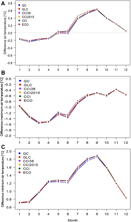
FIGURE 3. Annual cycle climatology (2002–2011) of the differences in 2-m temperature (A), maximum temperature (B) and minimum temperature (C) in the simulation experiments with land cover map GC (blue), GLC (red), CCI38 (purple), CCI 2015 (yellow), CCI (green), and ECO (brown) compared with the gridded observations. Please see Table 1 for abbreviations.

For maximum temperature, the simulations underestimate the highest temperature during the daytime down to −1.6°C in March. Minor discrepancies by −0.6°C occur during August through December. CCI38 is closest to the observations during April through July otherwise; ECO shows the least differences in maximum temperature.

Differences from observations are highest for minimum temperature. Here, the simulations overestimate the lowest temperature by +1.4°C to +1.85°C during nighttime, especially during July through October. The lowest discrepancies occur between December and February, and GC is closest to the observations, which is supported by the performance indices KGE and DAV (please see Supplementary Table S1 in supplementary material).

In summary, based on the results, strongest differences of the simulations results due to the land cover maps compared with observations are seen in maximum and minimum temperature during the vegetation period. Although the differences between model results and observations are small. It can be assumed that they are well within the uncertainty of the observations. Razafimaharo et al., 2020 calculated a mean temperature bias of HYRAS of ±0.03°C for meteorological sites and of ±0.8°C for gridded or monthly datasets.

Annual cycle differences in the 2-m, and maximum and minimum temperatures among the simulations are examined in Figures 4A–C. Here, the differences are calculated with respect to the control simulation based on GC (see Table 1). The 2-m temperature amplitude is highest for ECO/CCI38 with changes by approximately +0.04°C to +0.06°C for CCI38 with respect to GC in May through July and the lowest values are approximately −0.02°C to −0.03°C between January and March. ECO deviates by approximately +0.08°C to +0.04°C between June and August. The strongest differences are observed in maximum temperature at +0.1°C, which follows the pattern seen in the 2-m temperature (Figure 4B). The minimum temperature in the simulation experiments is higher than GC by up to +0.06°C over almost the entire year. Except in winter months, minimum temperatures are lower than GC by app. 0.02°C.

FIGURE 4

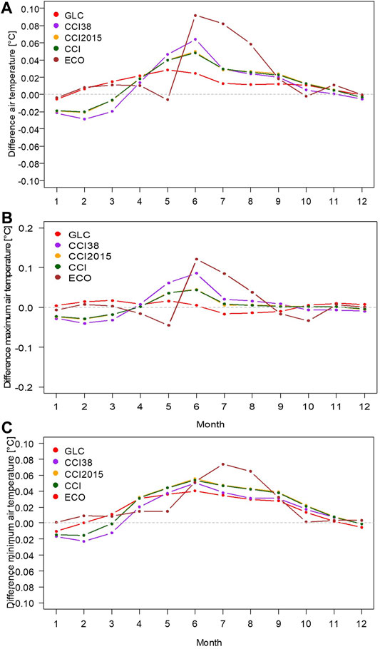
FIGURE 4. Annual cycle climatology (2002–2011) of the differences in 2-m temperature (A), maximum temperature (B) and minimum temperature (C) in the simulation experiments with land cover map GLC (red), CCI38 (purple), CCI 2015 (yellow), CCI (green), and ECO (brown) compared with the control simulation based on GC. Please see Table 1 for abbreviations.

The temperature differences among the simulations partly stem from changes seen in the vegetation parameters and finally latent heat fluxes, as demonstrated in Figures 5A–C. The smallest difference in LAI was −0.5 for CCI38 compared with GC during the vegetation period. Similarly, plant coverage was lower over the entire year compared with GC and further reduced down to −4 percent during the vegetation period. This reduction results in lower latent heat fluxes and finally higher temperatures. CCI and CCI2015 are very similar in their temperature discrepancies to GC following the amplitude of CCI38 but with a smaller magnitude. Both CCI and CCI2015 are very similar in their differences in LAI, plant coverage and latent heat fluxes (all are lower than GC) but of lesser magnitude than CCI38, which is seen in the smaller temperature difference. In contrast to CCI38, CCI and CCI2015 showed fewer plant cover differences (2%) during summer months than during winter months (3%). GLC is slightly warmer than GC by +0.02°C over most of the year. GLC has also the smallest LAI difference from GC. The picture is different for plant coverage, where GLC has a higher vegetation fraction than GC by up to +1 percent during June through August. Although GLC has lower LAI values than GC during summer months, the plant coverage is higher, which compensates for the lower LAI in transpiration during this period. A lower LAI together with a higher vegetation fraction results in nonsignificant differences from GC in the mean annual cycle of latent heat and reduced temperature differences. The picture for ECO is very different from the other land cover maps. The LAI of ECO deviates from GC with two cycles showing higher LAI values during spring and autumn, and lower values during summer months. Similarly, the PLCOV is higher in spring and autumn by up to 15% than GC. PLCOV is still higher with 6% during summer months. Accord to the annual LAI cycle, latent heat fluxes are increased in April and May and drop during summer. The different pattern seen in ECO is the result of the different land cover classification scheme.

FIGURE 5

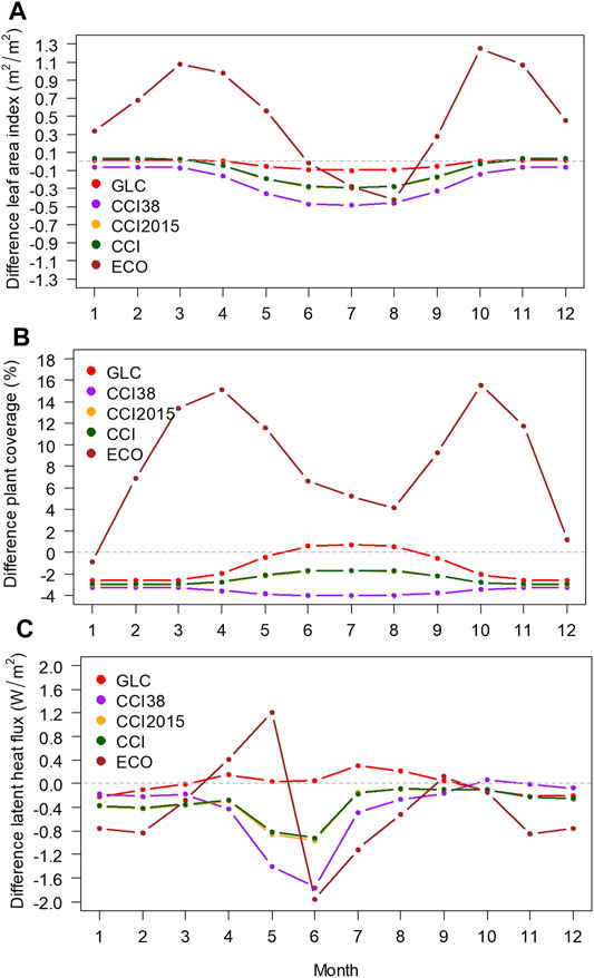
FIGURE 5. Annual cycle climatology (2002–2011) of the differences in leaf area index (A), plant coverage (B) and latent heat (C) in the simulation experiments with land cover map GLC (red), CCI38 (purple), CCI 2015 (yellow), CCI (green), and ECO (brown) compared with the control simulation based on GC. Please see Table 1 for abbreviations.

To summarize, differences in the annual cycle of temperature result from different land cover maps. The strongest changes between simulations occur in maximum temperature. The changes in temperature consistently relate to changes in LAI, plant coverage and latent heat fluxes. The results revealed that the largest differences occurred from spring to autumn, which was the main vegetation period in Germany due to climatic conditions. The comparison of the annual cycle over the entire simulation domain leads to compensation errors and hides regional differences due to spatial distribution changes in land cover classes.

The regionalization based on the 2-m temperature distribution of the simulation based on GC over the simulation domain is shown in Figure 6A as a climatological mean over the vegetation period (April to September) from 2002 to 2011. The influence of the topography is clearly visible. Temperature values range from 5°C in the south over the Alps to 21°C as discovered in the Rhine valley in the west. Hill ranges, such as the Black and Bavarian forests in the south, the forest of Thuringia in the east, the Rothaar Mountains in the central part of the domain, and the Harz in the north-east, are visible with temperatures ranging from 13°C to 15°C.

FIGURE 6

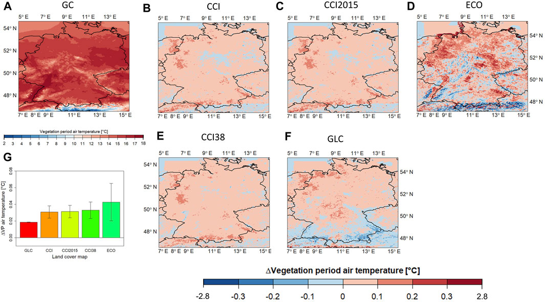
FIGURE 6. Distribution of daily vegetation period 2-m temperature climatology (2002–2011) for the control simulation based on GlobCover 2009 (A), the difference between the simulation based on CCI and the control simulation (B), the difference between the simulation based on CCI2015 and the control simulation (C), the difference between the simulation based on ECO and the control simulation (D), the difference between the simulation based on CCI38 and the control simulation (E), and the difference between the simulation based on GLC2000 and the control simulation (F). Domain averaged differences in vegetation period 2-m temperature for GLC, CCI, CCI 2015, CCI38, and ECO compared with the control simulation between 2002 and 2011 (G). Please see Table 1 for abbreviations. Grids with an overlaid black circle indicate statistically significant (at the 95th percentile level using the t-test) differences.

Temperature differences in the simulation experiment climatologies relative to GC are shown in Figures 6B–F, and their domain averaged temperature difference relative to GC in Figure 6G is summarized as a bar plot. ECO is the warmest compared with GC, followed by CCI38 and by both CCI and CCI 2015 (Figure 6G). Here, the differences in the spatial distribution are statistically significant (above the 95th percentile using the t-test). GLC has the smallest departure from GC, which is non-significant in the spatial distribution difference at the 95th percentile level using the t-test. ECO shows the highest variability in the temperature distribution and strongest differences. Marked warmer regions are seen in all the simulation experiments in the northwestern coastal area, in the Ruhr region (between 7°E and 9°E and 50°N to 53°N), compared with GC, and a colder region is depicted along the 52 and 53°N latitude. The alpine foreland in Southern Germany also shows warmer areas, up to +0.3°C, in the simulations based on the CCI. CCI38 shows most of the warmer areas. In contrast, colder regions are depicted for GLC (between −0.1 and −0.2°C) and ECO (up to 2.8°C cooler) in the alpine foreland in Southern Germany, Vorarlberg, Swiss and Austrian Alps. In the Swiss and Austrian Alps, valleys are generally warmer, and mountain tops cooler in ECO, which are statistically significant (above the 95th percentile using the t-test). Statistically significant differences, where ECO is cooler than GC, also occur in the Black Forest in the southeast of Germany, Liechtenstein and Vosges in the northeast of France. The large temperature difference seen between the ECO and the GC simulation (Figure 6D) in the northern coastal area over water is due to deviations in the land-sea mask. There is no land use in this region off the coast in GC. The soil type there is water and the temperature is determined by the SST analysis. These points are defined as land in the ECO simulation, which results in the differences seen. Land areas usually do not evaporate as much as open water areas at the same temperature leading to higher sensible heat fluxes (Supplementary Figure S2 in supplementary material).

Differences seen in the temperature distribution between the simulations stem from differences in the land cover class spatial distribution and fraction. Associated differences in the LAI, plant coverage, and latent heat fluxes result from these differences in land cover class spatial distribution and fraction (Figures 7A–O and Table 3). For example, the alpine foreland has more natural vegetation and pasture in GLC than GC (see Supplementary Figure S1 in supplementary material), which contributes to a climate that is cooler by app. 0.2°C in that area due to the higher LAI, plant cover and latent heat flux (Figure 7A,F,K). Here, the regression coefficients from linear regression analysis are negative between maximum temperature and natural vegetation fraction changes between GLC and GC (see Table 3). As natural vegetation fraction increases in GLC compared with GC, maximum temperature decreases and vice versa. GC has more crops in the alpine foreland with a lower LAI than natural vegetation. The cold bias in the south of the simulation domain of ECO results from higher LAI, plant cover and latent heat flux in that area compared to GC (Figures 7E,J,O), The simulations based on the CCI are generally warmer than GC with a distinct warmer area between 7°E and 9°E and 50°N to 53°N. This region is highly populated, known as the Ruhr area, with multiple cities and villages close to each other. The simulations based on CCI and ECO have more grid points with urban areas than GC in this region, contributing to the warming there (see also Figures 2A,B). The regression analysis (Table 4) reveals the greater the urban area fraction of the experiments compared to the reference simulation the higher the maximum temperature seen by the positive regression coefficient (positive change). The urban area fraction is increased in GLC, but also the pasture fraction. This is the reason why this region is not as warm as in the simulations based on the CCI. In central Germany along the 52 and 53°N latitude, there is more pasture than crops in all the experimental simulations, which results in a cooling effect. Linear regression results show a negative relationship between pasture fraction and maximum temperature (Table 4). More pasture than in GC results in a decrease in maximum temperature and vice versa. Another distinct warmer area is the northwestern coastal region. Here, the simulation experiments have less natural vegetation than in GC in association with lower LAI and latent heat fluxes (Figures 7A–E,K–O), which contributes to the warming in that area. The urban and crops fraction changes have the strongest impact on temperature changes during the vegetation period followed by pasture and then natural vegetation (see Table 4).

FIGURE 7

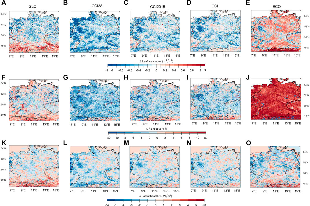
FIGURE 7. Distribution of latent heat flux (A–E), LAI (F–J), and plant cover (K–O) differences between the experimental simulation based on the GLC land cover map (first column), the CCI38 land cover map (second column), the CCI2015 land cover map (third column), the CCI land cover map (fourth column), the ECO land cover map (fifth column) and the control simulation based on the GC land cover map over the vegetation period (May to September) from 2002 to 2011. Please see Table 1 for abbreviations.

TABLE 3

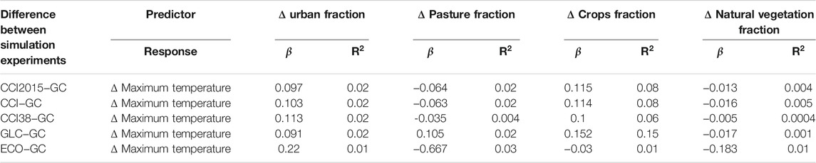
TABLE 3. Linear regression fit statistics for coefficient β and goodness-of-fit $R^2$ values between differences (experiment—control) in urban, pasture, crops and natural vegetation fraction as predictors and differences in maximum temperature as responses. All regression coefficients are statistically significant at p < 0.05. These statistics are calculated for each simulation experiment. Please see Table 1 for abbreviations of simulation experiments. Analysis is over the vegetation period (April to September).

TABLE 4

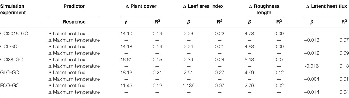
TABLE 4. Linear regression fit statistics for coefficient β and goodness-of-fit $R^2$ values between differences (experiment—control) in plant cover, leaf area index, roughness length as predictors and differences in latent heat as responses, and between differences in latent heat as predictor and differences in maximum temperature as responses. All regression coefficients are statistically significant at p < 0.05. These statistics are calculated for each simulation experiment. Please see Table 1 for abbreviations of simulation experiments. Analysis is over the vegetation period (April to September).

The influence of the surface parameters are see in the regionalization of daily maximum temperature differences over the simulation domain for the vegetation period as presented in Figures 8A–G. Generally, maximum temperature differences are larger than the average temperature changes. Maximum temperatures are increased in much of the Ruhr area and in the northwestern coastal region in the simulation experiments based on the CCI and ECO compared with the control simulation. Here, the land cover classes differ from the control simulation. The associated vegetation parameters determine the partitioning of energy between the sensible and latent heat fluxes in the model. Thus, the components of the daytime surface energy balance change as a result of land cover changes. This leads to differences in moisture availability in the grid cell. A lower LAI with a decreased vegetation fraction due to increased urban area fraction (see Figure 7 and linear regression analysis in Table 3 and Table 4) lead to a summer warming in the maximum temperature in the Ruhr region as evapotranspiration is reduced all summer (Figures 7K-O). Here, CCI38 is the warmest based on the domain average, whereas GLC temperature is close to that of GC. One of the reasons for the latter is that the spatial distribution and fraction of the urban area of GLC is close to that of GC (please see Figure 2 in this manuscript and Supplementary Figure S1 in the supplementary material). In contrast, the CCI data contain more grid cells with urban land cover. More urban grid points lead to larger sensible heat fluxes (Supplementary Figure S2 in the supplementary material) as latent heat fluxes are close to zero, which contributes to heating. The LAI is reduced in the northwestern coastal region, but the vegetation fraction is increased in some of the simulation experiments (GLC, CCI 2015, and CCI) at the same time (Figures 7A,C,D,F,H,I). Thus, the net impact on temperature is the result of the strength of these vegetation parameters influencing the evapotranspiration efficiency (Figures 7K,M,N). Note, that the daytime radiation flux via the surface albedo is not analyzed due to the constraints in the model (see Tölle et al., 2018 and Methodology section in this manuscript), where the albedo is described and does not depend on the different vegetation types or urban area.

FIGURE 8

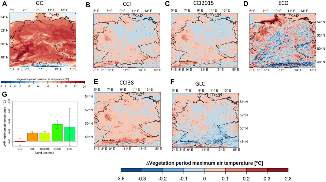
FIGURE 8. Distribution of daily vegetation period maximum temperature climatology (2002–2011) for the control simulation based on GlobCover 2009 (A), the difference between the simulation based on CCI and the control simulation (B), the difference between the simulation based on CCI2015 and the control simulation (C), the difference between the simulation based on ECO and the control simulation (D), the difference between the simulation based on CCI38 and the control simulation (E), and the difference between the simulation based on GLC2000 and the control simulation (F). Domain averaged differences in vegetation period maximum temperature for GLC, CCI, CCI 2015, CCI38, and ECO compared with the control simulation between 2002 and 2011 (G). Please see Table 1 for abbreviations. Grids with an overlaid black circle indicate statistically significant (at the 95th percentile level using the t-test) differences.

The relationship of the vegetation parameters (plant cover, leaf area index, roughness length) to the magnitude of latent heat flux and finally the latent heat flux impact on maximum temperature can be determined by linear regression analysis (Table 4). The positive influence of plant coverage is much stronger than the influence of the LAI based on the regression coefficients. The coefficient values (β) represent the mean change in the response of latent heat flux given a one unit change in one of the predictors (plant cover, LAI, or roughness length). For example, the coefficient for differences in the LAI is approximately +2, meaning that the mean response value (difference in latent heat) increases by approximately 2 for every one unit change in LAI difference (predictor). The linear regression with plant cover differences indicated the strongest response (coefficient values between 14 and 18), followed by Z0 with coefficient values approximately 5 and then LAI. However, the variability around the mean is best represented by the linear regression based on the LAI, as shown by the goodness-of-fit parameter ($R^2$) followed by plant coverage and then roughness length. Finally, the difference in latent heat fluxes results in differences in maximum temperature (negative relationship), but to a lesser extent than the influence of the vegetation parameters on latent heat flux changes. Here, the coefficients are negative. Thus, any grid cell showing a decrease in latent heat fluxes as shown in Figures 7A–F corresponds to an increase in maximum temperature and vice versa.

The strongest warming in the Ruhr region in the simulation experiments compared with GC is also dominant in the daily minimum temperature; see Figures 9A–F. All simulations show a comparable warming relative to GC and the most varbility is seen in ECO (Figure 9G). Minimum temperature is associated with the nocturnal surface energy balance. Higher temperatures during the daytime may result in enhanced storage of heat through thermal and radiative properties and higher roughness of cities, which leads to a warmer temperature at night in urban areas contributing to the urban heat island effect (Hamdi et al., 2020). Less vegetation and soil, and thus less evapotranspiration in urban areas decreases latent heat fluxes. This results in reduced loss of heat from the ground and impact daily minimum temperature. The radiative exchange may play a minor role in the nocturnal surface energy balance (Oke and Fuggle 1972), which is not examined here. The warming in the northwestern coastal region can be explained by changes in the vegetation class fractions. The other simulations experiments have less natural vegetation fractions in this area than GC. A decrease in LAI and evapotranspiration causes the warming here. The strongest cooling in minimum temperature in the alpine foreland, Vorarlberg, Liechtenstein, Swiss and Austrian Alps seen in GLC and ECO compared with GC is related to more natural vegetation and pasture in the area, leading to increases in LAI and vegetation fraction and thus latent heat fluxes. Here, less storage of heat during the daytime via evaporative cooling leads to a cooler temperature at night. Enhanced emissivity could also explain the cooling there. Overall, the warmest nights based on the domain average are seen in both the CCI and CCI 2015.

FIGURE 9

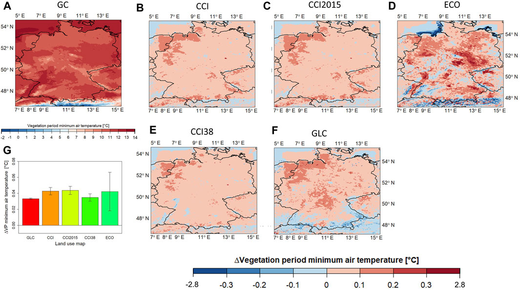
FIGURE 9. Distribution of daily vegetation period minimum temperature climatology (2002–2011) for the control simulation based on GlobCover 2009 (A), the difference between the simulation based on CCI and the control simulation (B), the difference between the simulation based on CCI2015 and the control simulation (C), the difference between the simulation based on ECO and the control simulation (D), the difference between the simulation based on CCI38 and the control simulation (E), and the difference between the simulation based on GLC2000 and the control simulation (F). Domain averaged differences in vegetation period minimum temperature for GLC, CCI, CCI 2015, CCI38, and ECO compared with the control simulation between 2002 and 2011 (G). Please see Table 1 for abbreviations. Grids with an overlaid black circle indicate statistically significant (at the 95th percentile level using the t-test) differences.

To summarize, the fraction and spatial distribution changes in land cover classes over the domain are relevant in determining the regional and local water fluxes and temperature climate in a region. The land cover classes in the northwest coastal and Ruhr regions, along the 52 and 53° N latitude and in the alpine foreland differ considerable between the land cover maps. GC has more natural vegetation in the northwest coastal region than the other land cover maps. The region between Germany and Switzerland, and between Germany and Austria have more pasture in the CCI data than in GC. GLC and ECO have more forest and pasture. In contrast, GC shows more crops in these areas. All of the land cover maps have increased urban fraction especially in the Ruhr region than GC. More pasture is depicted along the 52 and 53° N latitude in all of the land cover maps than in GC. These differences are seen in the climate variables, although of small magnitude. The associated changes in LAI and plant coverage explain a major part of the surface latent heat and temperature differences. The differences in the LAI, plant coverage and roughness length ultimately change the amount of latent heat flux to the atmosphere. Maximum and minimum temperatures enable a direct evaluation of the physical processes of the surface energy balance. Maximum temperature is most affected by the differences in land cover classes, whose changes are of the highest magnitude. Therefore, further analysis is based on maximum temperature. Higher latent heat fluxes result in evaporative cooling and lower latent heat fluxes have reduced cooling efficiency, which is seen in the temperature changes.

The daily maximum temperature difference climatology for grid cells, where a dominant (more than 40%) land cover type change occurs, is presented in Figures 10A–E and summarized as boxplots for each month of the year from 2002 to 2011. Differences in land cover types are calculated between CCI 2015, CCI, CCI38, ECO and GLC (experiments) and GC (control). In May and June, the highest increase in maximum temperature (∼0.2°C in the median) is due to the land cover change results for the grid cells, where natural vegetation is converted to urban areas. This means that grid cells, which were dominated by natural vegetation or pasture in the GC simulation, were urban areas in the experimental simulations. Accordingly, the maximum temperature is lower over those grid cells in GC than in the experiments over urban areas resulting in a positive change. The lower evapotranspiration in urban areas by 8–12 W/m² in the median (see Figures 11A–E) causes larger sensible heat fluxes by 4–8 W/m² in the median (see Supplementary Figure S3 in supplementary material), which lead to an increased temperature. The most pronounced changes were observed for ECO and CCI38, followed by CCI 2015, CCI and GLC. Changes from natural vegetation to cropland or pasture also show a considerable positive maximum temperature change. Here, the evapotranspiration is lower for croplands and pasture than for natural vegetation in the model (Figures 11A–E), which results in warmer temperatures. Based on the t-value computed using the two-sided t-test, the warming signal is statistically significant at the 95th percentile level (i.e., t-value of more than 2) in June for grid cells converted from natural vegetation to urban areas, from natural vegetation to pasture or from natural vegetation to crops. The cropland change into pasture type causes slightly higher temperatures during the summer months, but with high variability. In this case, the decreased soil moisture (not shown) is an additional reason for the increased temperature, apart from evapotranspiration changes, as a result of the higher evapotranspiration. From October to March, negligible changes (mostly negative with a small magnitude) occur. Changes from cropland to urban areas have a minor impact on maximum temperature, which is a positive change.

FIGURE 10

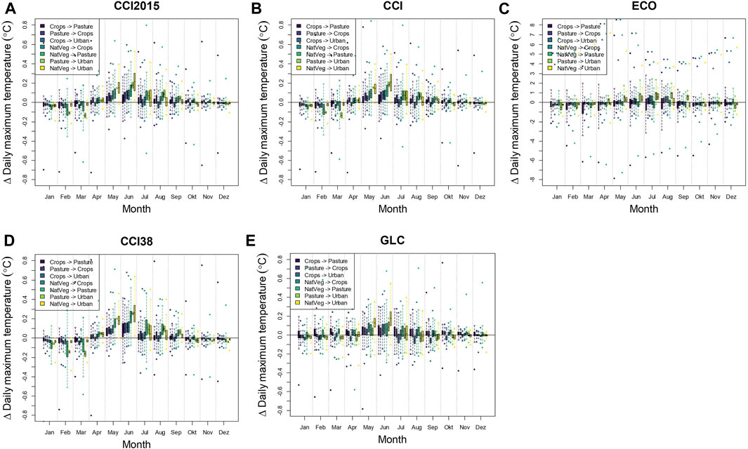
FIGURE 10. Monthly differences in daily maximum temperature due to dominant land cover changes (more than 40%) between CCI2015 and GC (A), CCI and GC (B), ECO and GC (C), CCI38 and GC (D), and GLC and GC (E) for the time period from 2002 to 2011. Cropland grid cells change into pasture type (purple), pasture grid cells change into crops (dark blue), crop grid cells change into urban type (blue), natural vegetation grid cells change into crop type (dark green), natural vegetation grid cells change into pasture type (green), pasture grid cells change into urban type (light green), and natural vegetation grid cells change into urban type (yellow). Differences are calculated for grid cells, where the listed land cover type change occurs. Please see Table 1 for abbreviations of simulation experiments.

FIGURE 11

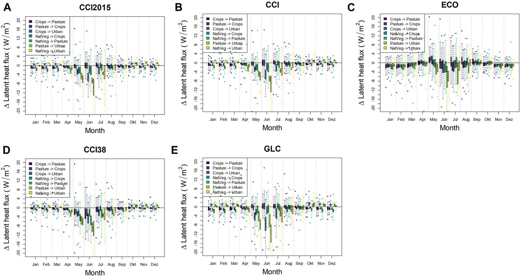
FIGURE 11. Monthly differences in daily latent heat flux due to dominant land cover changes (more than 40%) between CCI2015 and GC (A), CCI and GC (B), ECO and GC (C), CCI38 and GC (D), and GLC and GC (E) for the time period from 2002 to 2011. Cropland grid cells change into pasture type (purple), pasture grid cells change into crops (dark blue), crop grid cells change into urban type (blue), natural vegetation grid cells change into crop type (dark green), natural vegetation grid cells change into pasture type (green), pasture grid cells change into urban type (light green), and natural vegetation grid cells change into urban type (yellow). Differences are calculated for grid cells, where the listed land cover type change occurs. Please see Table 1 for abbreviations of simulation experiments.

The climatology of differences in climate indices due to land cover change is shown in Figures 12A–E summarized as a boxplot for each climate index from 2002 to 2011. The greatest differences are seen for any land cover type change to urban areas. For example, tropical nights are less in the GC simulation over natural vegetation or pasture compared with that over urban areas resulting in a positive change. Accordingly, summer days are increased in urban areas. Ice days (IDs) are increased by up to 10 days due to changes from natural vegetation to pasture. However, frost and ice days are either decreased or increased depending on the land cover map. One explanation could be that IDs are increased in urban areas, as concrete can hold heat less than wooded areas. The temperature is influenced by the thermal properties, which specifies the behavior in storing and releasing heat. The heat capacity of wood (1.76 J/g°C) is approximately double that of concrete or brick (0.88 J/g°C). Similarly, this effect also results in increased FDs due to land cover change to the urban type. The growing season length (GSL) is shortened by 0.6 days at the median for any change to urban areas. The growing season start (GSS) can be delayed by up to 1.6 days due to a change in urban areas, as in the case of CCI 2015. Both indices show high variability. Overall, the greatest differences are shown for ECO and CCI 2015, followed by CCI and CCI38. The least changes are found for GLC.

FIGURE 12

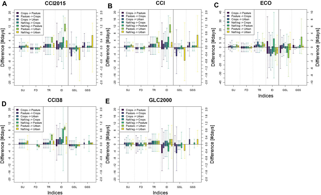
FIGURE 12. Differences of climate indices in days due to land cover change between CCI2015 and GC (A), CCI and GC (B), ECO and GC (C), CCI38 and GC (D), and GLC and GC (E) for the time period from 2002 to 2011. Cropland grid cells change into pasture type (purple), pasture grid cells change into cropland (dark blue), cropland grid cells change into urban type (blue), natural vegetation grid cells change into crop type (dark green), natural vegetation grid cells change into pasture type (green), pasture grid cells change into urban type (light green), and natural vegetation grid cells change into urban type (yellow). Differences are calculated for grid cells, where the listed land cover type change occurs. The climate indices are Summer Days (SU), Frost Days (FD), Tropical Nights (TR), Ice Days (ID), Growing Season Length (GSL), and Growing Season Start (GSS). Please see Table 1 for abbreviations of simulation experiments.

In summary, daily maximum temperature difference was calculated for grid cells where a land cover type change occurred. The results revealed higher daily maximum temperatures in May and June if natural vegetation or pasture grid cells changed to urban types followed by natural vegetation changes to pasture or crops. CCI data showed the strongest impact. Greatest differences in climate extremes were seen for any land cover types that changed to urban areas, resulting in more ID or FD days in urban areas due to the differences in thermal and radiative properties and thus heat capacity. SU and TR days increased with a land cover change from natural vegetation to urban.

Discussion and Conclusions

Many modelling studies have revealed the importance of land cover changes to climate in different regions worldwide, mostly based on idealized land cover change studies and coarse horizontal resolution (e.g., Tölle et al., 2017; Cherubini et al., 2018; Davin et al., 2020). Only a few studies have examined the effects of more realistic anthropogenic land cover changes on climate (Heck et al., 2001; Huang et al., 2020), and on convection-permitting scales (Tölle et al., 2014; Prein et al., 2015). Convection-permitting scales (<4 km) allow the analysis of local scale impacts. The land cover map is an input to the land surface model, which provides the lower boundary conditions (e.g., in terms of fluxes) to the atmospheric model. However, the impact of the various land cover map products on regional and local climate has thus far been less investigated. Only a few studies have investigated specific land cover databases (Masson et al., 2003; Bontemps et al., 2012). There is the need to update this information based on the newly available products, such as CCI data. All the land cover maps have different land cover classes and amounts and differ in terms of horizontal resolution and retrieval year. These discrepancies eventually lead to differences in land cover class spatial distribution and fraction over the study region.

Here we quantified the climate uncertainty due to different land cover maps in the regional climate model CCLM (Rockel et al., 2008). We performed convection-permitting simulations (Ban et al., 2021) at 3 km spatial resolution driven by ERA5 reanalysis data over Germany and adjacent areas. By analyzing the simulations from 2002 to 2011 we investigated in land cover changes due to the retrieval year of the land cover maps, number, fraction and spatial distribution of land cover classes. The comparison results to observations revealed a 2-m temperature bias between −0.2 (Feb) and +0.6°C (Sep) in the annual cycle. The maximum temperature is generally colder than the observations, ranging from −1.6°C (Feb-Mar) to −0.3°C (Sep–Nov). Schulz et al. (2020) have shown that the total latent heat flux is overestimated in the current model version leading to the systematic underestimation of maximum temperature. The authors found that the bias can be reduced by implementing a new scheme for bare soil evaporation based on a resistance formulation. The minimum temperature is generally warmer throughout the year, ranging from +0.7°C (Feb) to +1.9°C (Sep). The nocturnal warm bias can be systematically reduced by accounting for skin temperature as demonstrated by Schulz et al. (2020). However, the small differences between model results and observations are well within the uncertainty of the observations (see Razafimaharo et al., 2020).

Furthermore, differences in the annual cycle of temperature result from different land cover maps and mostly appear during the vegetation period (April to September), but the impact is less strong than the bias to the observations. The parameterization schemes in the model determine the bias to the observations during nighttime rather than the differences in land surface parameters and need improvements (Prein et al., 2015).

The small impact due to different land cover maps depends on the study region. Masson et al. (2003), using the climate model ARPEGE based on the new ECOLCIMAP and old surface parameters, showed that the impact over central Europe is low, but could reach values up to +5°C in other regions of the world (e.g., Greenland, western US, southern edge of South America, and the Himalayas). Their study showed that the spatial consistency of global datasets is characterized by spatial heterogeneity that is, there is no consistency of different regions. It would be interesting to repeat this study over hotspot areas of climate change (e.g., the Mediterranean or Arctic region). For example, a misrepresentation of the vegetation cover over Iberia can reach a temperature bias of up to 10°C (Nogueira et al., 2020).

According to the comparison and analyses in this study, the spatial consistency was high among the simulations with different land cover maps compared to observations. This finding is not surprising as the land cover class fractional differences were small among the land cover maps. However, some land cover types, such as croplands and urban areas, have greatly changed over the years. The land cover based on GLC is the oldest among the land cover datasets. Here, the crop area was still higher than that in GC. This difference is also seen in the temperature differences, although they are of small magnitude. The land cover classes in the northwestern coastal and Ruhr regions, along the 52 and 53°N latitude and in the alpine foreland, Vorarlberg, Liechtenstein, Swiss and Austrian Alps differed considerable between the land cover maps. These differences were seen in the climate variables. The same land cover map products based on the CCI of different years (2000 and 2015) revealed no accreditable difference in the climate variables. The land cover changes that occurred between these years are marginal and thus, the influence is small over Germany. However, maintaining temporal consistency would be useful for areas with major land cover changes. This consistency can still be critical for smaller regions, where urban areas increase, or for hotspots of land cover changes (e.g. deforestation). Increasing the land cover types, as in CCI38 or ECO, leads to higher temperature variability. Thus, using more land cover classes may show heterogeneities among regions, as land cover changes in local areas could be dramatic. If the land cover maps based on ECOCLIMAP is favorable due to more land cover classes in the alpine foreland, Vorarlberg, Liechtenstein, Swiss and Austrian Alps needs to be determined.

Even though the spatial discrepancies in temperature among the simulations due to the different land cover maps were small in magnitude, they were consistent and could be explained by the processes and differences in the surface characteristics. The small differences seen in our simulations relate to changes in the surface parameters due to differences in land cover types. The components of the surface energy balance change as a result of the different surface parameters. This effect leads to different moisture availabilities in grid cells. The results revealed that the largest differences occurred from spring to autumn, which was the main vegetation period in Germany due to climatic conditions. The strongest changes between the simulations occur in maximum temperature. The changes in temperature are related to changes in the LAI, plant coverage, roughness length and latent heat fluxes. The vegetation fraction was the main parameter affecting the seasonal evolution of the latent heat fluxes based on linear regression analysis, followed by the roughness length and the LAI. Other studies outline the stronger importance of the LAI (Tölle et al., 2014; Forero Urrego et al., 2021) or roughness length (Breil et al., 2021) on the latent heat fluxes or temperature. Our results clearly indicate the plant coverage is the most important factor for evapotranspiration. This result can be confirmed by evapotranspiration calculations in the regional climate model (Doms et al., 2013). The evaporation terms of the interception reservoir, bare soil, and transpiration all depend on plant coverage. However, there is a reciprocal dependency of these terms on roughness length, and the transpiration calculation is the only one that depends on the LAI. However, these model equations need to be revisited and updated. Accounting for specific plant species and land surface covers would be beneficial.

Distinct spatial distribution differences among the simulations with the different land cover maps leading to local and regional temperature changes could be determined from our analysis. The analysis based on the CCI and ECO data revealed the strongest warming impact. The CCI data have a higher urban fraction than GLC or GC. The presentation of the urban and built-up areas is also higher and more detailed in the ECO data, including impervious surfaces, such as streets. Therefore, the fraction of urban area is increased in both of these databases, leading to a stronger warming. The daily maximum temperature difference between the simulations was calculated for grid cells where a land cover type change occurred. The strongest effect was seen if natural vegetation or pasture grid cells changed to urban types followed by natural vegetation changes to pasture or crops, which resulted in higher daily maximum temperatures in May and June. The variability seen with these differences could partly stem from inconsistencies between the land cover and albedo input data. Both are prescribed by external fields in the model and might not perfectly match with each other. This is an important issue regarding local scale impact analysis. These results strengthen the need for the correct mapping of land cover classes, which is needed for impact studies and forecasts. Several recent studies among other regions in the world called for the same conclusion (see for example Cao et al., 2015; Bhati and Mohan, 2018; Li et al., 2020; López-Espinoza et al., 2020; Glotfelty et al., 2021; Golzio et al., 2021).

Dominant land cover changes between the land cover datasets result in differences in climate extremes. The greatest differences were seen for any land cover types that changed to urban areas, resulting in more ID or FD days in urban areas due to the differences in thermal and radiative properties and thus heat capacity. SU and TR days increased with a land cover change from natural vegetation to urban. The climate model version in this study represents urban areas as natural land surfaces only. Thus, the impact of cities might be underestimated as Katzfey et al., (2020) and Daniel et al. (2018) have shown for a global and regional study respectively. Including more sophisticated urban schemes in convection-permitting climate model simulations, as demonstrated by Raffa et al. (2021), de Wit et al. (2020) and Hertwig et al. (2020), should be the way forward.

This study showed that there are spatial inconsistencies in land cover datasets leading to differences in local and regional climate. The spatiotemporal heterogeneity in surface parameters in weather and climate models is considered to be a key component of the partitioning of the water and energy fluxes influencing regional and local climate. This factor has a significant impact on multiple research fields including regional climate change studies, hydrological forecasting for watersheds, meteorological forecasts, and drought monitoring and forecasting for agriculture and forestry industries. The spatial resolution will increase in the future. Thus, other land cover datasets with higher spatial resolution, such as GlobeLand30, which has a resolution of 30 m, would be beneficial to use in climate and land management studies by including more land cover classes. Additional land cover classes increase the variability in the climate as revealed from our analysis. This factor would also enable a more realistic representation of the climates between transition zones (e.g., city and countryside or transition zone between urban and rural areas). There are hotspots of land cover change driven by agricultural expansion or population growth, which might require additional land cover types and information for their changes. Although the development of land cover datasets greatly promotes scientific research, satisfying the needs of high-precision land-surface-process simulations remains difficult. More attention should be given to land cover classification in complex areas and regional representative classification sample selection for future development of land cover datasets. Accounting for single vegetation species might also be relevant for management purposes.

The observed uncertainties in regional temperature due to different land cover datasets were overall lower than the uncertainties associated with climate projections based on anthropogenic emissions of greenhouse gases represented by the Radiative Concentration Pathways (RCPs, Meinshausen et al., 2011). Although local effects on climate due to changes to urban areas could be stronger or comparable to the RCPs. As the study has shown, the impacts and their implications are different on different spatial and temporal scales.

Thus, representation of urban areas, including single plant species especially for agricultural areas and synchronized input data will improve climate simulations at local scales. Accounting for sophisticated urban and vegetation parameterization schemes would be beneficial in land cover change and management studies with convection-permitting regional climate models for climate adaptation strategies.

Data Availability Statement

The original contributions presented in the study are included in the article/Supplementary Material, further inquiries can be directed to the corresponding author. Part of the analysis code can be accessed via GitHub: https://github.com/EvgenyChur/Land-cover-maps.

Author Contributions

MT acquired the funding, designed and conducted the experiments. MT performed the analysis and obtained the statistical results. EC contributed to evaluation statistics. MT wrote the manuscript. EC contributed to writing about the performance indices. All authors helped in revising the manuscript. All authors agree to be accountable for the content of the work.

Funding

This research was funded by the German Research Foundation (DFG) through grant number 401857120 and MAPPY. The MAPPY project is part of AXIS, an ERA-NET initiated by JPI Climate, and funded by FFG (Austria), F.R.S.-FNRS and BELSPO (Belgium), DLR/BMBF (Germany), NWO (Netherlands) and AEI (Spain) with co-funding by the European Union (Grant No. 776608, Funding reference No. 01LS1903C). Computational resources were made available by the German Climate Computing Center (DKRZ) through support from the German Federal Ministry of Education and Research (BMBF). This research was conducted in collaboration with the CLM-community.

Conflict of Interest

The authors declare that the research was conducted in the absence of any commercial or financial relationships that could be construed as a potential conflict of interest.

Publisher’s Note

All claims expressed in this article are solely those of the authors and do not necessarily represent those of their affiliated organizations, or those of the publisher, the editors and the reviewers. Any product that may be evaluated in this article, or claim that may be made by its manufacturer, is not guaranteed or endorsed by the publisher.

Acknowledgments

We thank Jürgen Helmert for consultancy.

Supplementary Material

The Supplementary Material for this article can be found online at: https://www.frontiersin.org/articles/10.3389/feart.2021.722244/full#supplementary-material

References

Arakawa, A., and Lamb, V. R. (1977). “Computational Design of the Basic Dynamical Processes of the UCLA General Circulation Model,” in Methods in Computational Physics: General Circulation Models of the Atmosphere. Editor J. Chang (New York, NY, USA: Academic Press), 17, 173–265. doi:10.1016/B978-0-12-460817-7.50009-4

CrossRef Full Text | Google Scholar

Arino, O., Bicheron, P., Achard, F., Latham, J., Witt, R., and Weber, J. L. (2008). GLOBCOVER the Most Detailed Portrait of Earth. ESA Bull.-Eur. Space 136, 24–31.

Google Scholar

Baldauf, M., Seifert, A., Förstner, J., Majewski, D., Raschendorfer, M., and Reinhardt, T. (2011). Operational Convective-Scale Numerical Weather Prediction with the COSMO Model: Description and Sensitivities. Mon. Weather Rev. 139, 3887–3905. doi:10.1175/mwr-d-10-05013.1

CrossRef Full Text | Google Scholar

Ban, N., Caillaud, C., Coppola, E., Pichelli, E., Sobolowski, S., Adinolfi, M., et al. (2021). The First Multi-Model Ensemble of Regional Climate Simulations at Kilometer-Scale Resolution, Part I: Evaluation of Precipitation. Clim. Dyn. 57, 275–302. doi:10.1007/s00382-021-05708-w

CrossRef Full Text | Google Scholar

Barrett, A. I., Gray, S. L., Kirshbaum, D. J., Roberts, N. M., Schultz, D. M., and Fairman, J. G. (2015). Synoptic versus Orographic Control on Stationary Convective Banding. Q.J.R. Meteorol. Soc. 141, 1101–1113. doi:10.1002/qj.2409

CrossRef Full Text | Google Scholar

Bartholomé, E., and Belward, A. S. (2005). GLC2000: a New Approach to Global Land Cover Mapping from Earth Observation Data. Int. J. Remote Sensing 26, 1959–1977. doi:10.1080/01431160412331291297

CrossRef Full Text | Google Scholar

Belušić, D., Fuentes-Franco, R., Strandberg, G., and Jukimenko, A. (2019). Afforestation Reduces Cyclone Intensity and Precipitation Extremes over Europe. Environ. Res. Lett. 14, 074009. doi:10.1088/1748-9326/ab23b2

CrossRef Full Text | Google Scholar

Betts, R. (2007). Implications of Land Ecosystem-Atmosphere Interactions for Strategies for Climate Change Adaptation and Mitigation. Tellus B: Chem. Phys. Meteorology 59, 602–615. doi:10.1111/j.1600-0889.2007.00284.x

CrossRef Full Text | Google Scholar

Bhati, S., and Mohan, M. (2018). WRF-urban Canopy Model Evaluation for the Assessment of Heat Island and thermal comfort over an Urban Airshed in India under Varying Land Use/land Cover Conditions. Geosci. Lett. 5, 27. doi:10.1186/s40562-018-0126-7

CrossRef Full Text | Google Scholar

Bontemps, S., Herold, M., Kooistra, L., van Groenestijn, A., Hartley, A., Arino, O., et al. (2012). Revisiting Land Cover Observation to Address the Needs of the Climate Modeling Community. Biogeosciences 9, 2145–2157. doi:10.5194/bg-9-2145-2012

CrossRef Full Text | Google Scholar

Breil, M., Davin, E. L., and Rechid, D. (2021). What Determines the Sign of the Evapotranspiration Response to Afforestation in European Summer? Biogeosciences 18 (4), 1499–1510. doi:10.5194/bg-18-1499-2021

CrossRef Full Text | Google Scholar

Brovkin, V., Sitch, S., Von Bloh, W., Claussen, M., Bauer, E., and Cramer, W. (2004). Role of Land Cover Changes for Atmospheric CO2 Increase and Climate Change during the Last 150 Years. Glob. Change Biol. 10, 1253–1266. doi:10.1111/j.1365-2486.2004.00812.x

CrossRef Full Text | Google Scholar

Cao, Q., Yu, D., Georgescu, M., Han, Z., and Wu, J. (2015). Impacts of Land Use and Land Cover Change on Regional Climate: a Case Study in the Agro-Pastoral Transitional Zone of China. Environ. Res. Lett. 10, 124025. doi:10.1088/1748-9326/10/12/124025

CrossRef Full Text | Google Scholar

CEC (1993). CORINE Land Cover Technical Guide. Luxembourg: European Union, Directorate-Environment.

Google Scholar

Champeaux, J.-L., Arcos, D., Bazile, E., Giard, D., Goutorbe, J.-P., Habets, F., et al. (2000). AVHRR-derived Vegetation Mapping over Western Europe for Use in Numerical Weather Prediction Models. Int. J. Remote Sensing 21, 1183–1199. doi:10.1080/014311600210137

CrossRef Full Text | Google Scholar

Champeaux, J. L., Masson, V., and Chauvin, F. (2005). ECOCLIMAP: a Global Database of Land Surface Parameters at 1 Km Resolution. Meteorol. Appl. 12, 29–32. doi:10.1017/S1350482705001519

CrossRef Full Text | Google Scholar

Cherubini, F., Huang, B., Hu, X., Tölle, M. H., and Strømman, A. H. (2018). Quantifying the Climate Response to Extreme Land Cover Changes in Europe with a Regional Model. Environ. Res. Lett. 13, 074002. doi:10.1088/1748-9326/aac794

CrossRef Full Text | Google Scholar

Coppola, E., Sobolowski, S., Pichelli, E., Raffaele, F., Ahrens, B., Anders, I., et al. (2018). A First-Of-Its-Kind Multi-Model Convection Permitting Ensemble for Investigating Convective Phenomena over Europe and the Mediterranean. Clim. Dyn. 55, 3–34. doi:10.1007/s00382-018-4521-8

CrossRef Full Text | Google Scholar

Daniel, M., Lemonsu, A., Déqué, M., Somot, S., Alias, A., and Masson, V. (2018). Benefits of Explicit Urban Parameterization in Regional Climate Modeling to Study Climate and City Interactions. Clim. Dyn. 52, 2745–2764. doi:10.1007/s00382-018-4289-x

CrossRef Full Text | Google Scholar

Davin, E. L., Rechid, D., Breil, M., Cardoso, R. M., Coppola, E., Hoffmann, P., et al. (2020). Biogeophysical Impacts of Forestation in Europe: First Results from the LUCAS (Land Use and Climate across Scales) Regional Climate Model Intercomparison. Earth Syst. Dynam. 11, 183–200. doi:10.5194/esd-11-183-2020

CrossRef Full Text | Google Scholar

de Noblet-Ducoudré, N., Boisier, J.-P., Pitman, A., Bonan, G. B., Brovkin, V., Cruz, F., et al. (2012). Determining Robust Impacts of Land-Use-Induced Land Cover Changes on Surface Climate over North America and Eurasia: Results from the First Set of LUCID Experiments. J. Clim. 25, 3261–3281. doi:10.1175/JCLI-D-11-00338.1

CrossRef Full Text | Google Scholar

de Noblet-Ducoudré, N., and Pitman, A. J. (2021). Terrestrial Processes and Their Roles in Climate Change. Clim. Sci.. doi:10.1093/acrefore/9780190228620.013.825

CrossRef Full Text | Google Scholar

de Wit, R., Kainz, A., Goler, R., Žuvela-Aloise, M., Hahn, C., Zuccaro, G., et al. (2020). Supporting Climate Proof Planning with CLARITY's Climate Service and Modelling of Climate Adaptation Strategies - the Linz Use-Case. Urban Clim. 34, 100675. doi:10.1016/j.uclim.2020.100675

CrossRef Full Text | Google Scholar

Di Gregorio, A., and Jansen, L. (2000). Land Cover Classification System (LCCS): Classification Concepts and User Manual. Rome: Italy.

Google Scholar

Dickinson, R. E. (1984). Modeling Evapotranspiration for Three-Dimensional Global Climate Models. Maurice Ewing 5 5, 58–72. doi:10.1029/gm029p0058

CrossRef Full Text | Google Scholar

Doms, G., and Baldauf, M. (2013). A Description of the Non-hydrostatic Regional COSMO Model, Part I: Dynamics and Numerics; Offenbach: Germany. Available at: http://www.cosmo-model.org/content/model/general/dynamics.htm (accessed April 25, 2021).

Google Scholar

Doms, G., Förster, J., Heise, E., Herzog, H.-J., Mironov, D., Raschendorfer, M., et al. (2013). A Description Of the Non-hydrostatic Regional COSMO Model, Part II: Physical Parameterizations; Offenbach: Germany. Available at: https://www.dwd.de/EN/ourservices/cosmo_documentation/pdf_docu_v5_0/2_cosmo_physics_5_00.pdf?__blob=publicationFile&v=3 (accessed April, 202125).

Google Scholar

FAO (1988). FAO-UNESCO Soil Map of the World. Revised Legend. FAO/UNESCO/ISRIC World Soil Resources Reports No. 60.

Google Scholar

Fischer, G., Nachtergaele, F., Prieler, S., van Velthuizen, H. T., Verelst, L., and Wiberg, D. (2008). Global Agro-Ecological Zones Assessment For Agriculture (GAEZ 2008). Rome, Italy: IIASA, Laxenburg, Austria and FAO.

Google Scholar

Friedl, M. A., Sulla-Menashe, D., Tan, B., Schneider, A., Ramankutty, N., Sibley, A., et al. (2010). MODIS Collection 5 Global Land Cover: Algorithm Refinements and Characterization of New Datasets. Remote Sensing Environ. 114, 168–182. doi:10.1016/j.rse.2009.08.016

CrossRef Full Text | Google Scholar

Garnaud, C., Sushama, L., and Verseghy, D. (2015). Impact of Interactive Vegetation Phenology on the Canadian RCM Simulated Climate over North America. Clim. Dyn. 45, 1471–1492. doi:10.1007/s00382-014-2397-9

CrossRef Full Text | Google Scholar

Glotfelty, T., Ramírez-Mejía, D., Bowden, J., Ghilardi, A., and West, J. J. (2021). Limitations of WRF Land Surface Models for Simulating Land Use and Land Cover Change in Sub-saharan Africa and Development of an Improved Model (CLM-AF V. 1.0). Geosci. Model. Dev. 14, 3215–3249. doi:10.5194/gmd-14-3215-2021

CrossRef Full Text | Google Scholar

Golzio, A., Ferrarese, S., Cassardo, C., Diolaiuti, G. A., and Pelfini, M. (2021). Land-Use Improvements in the Weather Research and Forecasting Model over Complex Mountainous Terrain and Comparison of Different Grid Sizes. Boundary-layer Meteorol. 180, 319–351. doi:10.1007/s10546-021-00617-1

CrossRef Full Text | Google Scholar

Gupta, H. V., Kling, H., Yilmaz, K. K., and Martinez, G. F. (2009). Decomposition of the Mean Squared Error and NSE Performance Criteria: Implications for Improving Hydrological Modelling. J. Hydrol. 377, 80–91. doi:10.1016/j.jhydrol.2009.08.003

CrossRef Full Text | Google Scholar

Hamdi, R., Kusaka, H., Doan, Q.-V., Cai, P., He, H., Luo, G., et al. (2020). The State-Of-The-Art of Urban Climate Change Modeling and Observations. Earth Syst. Environ. 4, 631–646. doi:10.1007/s41748-020-00193-3

CrossRef Full Text | Google Scholar

Hansen, M. C., DeFries, R. S., Townshend, J. R. G., and Sohlberg, R. (2000). Global Land Cover Classification at 1 Km Spatial Resolution Using a Classification Tree Approach. Int. J. Remote Sensing 21, 1331–1364. doi:10.1080/014311600210209

CrossRef Full Text | Google Scholar

Heck, P., Lüthi, D., Wernli, H., and Schär, C. (2001). Climate Impacts of European-Scale Anthropogenic Vegetation Changes: A Sensitivity Study Using a Regional Climate Model. J. Geophys. Res. 106, 7817–7835. doi:10.1029/2000jd900673

CrossRef Full Text | Google Scholar

Heret, C., Tittebrand, A., and Berger, F. H. (2006). Latent Heat Fluxes Simulated with a Non-hydrostatic Weather Forecast Model Using Actual Surface Properties from Measurements and Remote Sensing. Boundary-layer Meteorol. 121, 175–194. doi:10.1007/s10546-006-9104-2

CrossRef Full Text | Google Scholar

Hersbach, H., de Rosnay, P., Bell, B., Schepers, D., Simmons, A., Soci, C., et al. (2018). Operational Global Reanalysis: Progress, Future Directions And Synergies With NWP; ERA Report Series 27. Reading, UK: ECMWF.

Google Scholar

Hertwig, D., Grimmond, S., Hendry, M. A., Saunders, B., Wang, Z., Jeoffrion, M., et al. (2020). Urban Signals in High-Resolution Weather and Climate Simulations: Role of Urban Land-Surface Characterisation. Theor. Appl. Climatol. 142, 701–728. doi:10.1007/s00704-020-03294-1

CrossRef Full Text | Google Scholar

Heymann, Y. (1993). CORINE Land Cover: Technical Guide. Environment, Nuclear Safety and Civil protection Series, Commission of the European Communities. Luxembourg: Office for Official Publication of the European Communities, 144.

Google Scholar

Hohenegger, C., Brockhaus, P., Bretherton, C. S., and Schär, C. (2009). The Soil Moisture-Precipitation Feedback in Simulations with Explicit and Parameterized Convection. J. Clim. 22 (19), 5003–5020. doi:10.1175/2009JCLI2604.1

CrossRef Full Text | Google Scholar

Hua, T., Zhao, W., Liu, Y., Wang, S., and Yang, S. (2018). Spatial Consistency Assessments for Global Land-Cover Datasets: A Comparison Among GLC2000, CCI LC, MCD12, GLOBCOVER and GLCNMO. Remote Sensing 10 (11), 1846. doi:10.3390/rs10111846

CrossRef Full Text | Google Scholar

Huang, B., Hu, X., Fuglstad, G.-A., Zhou, X., Zhao, W., and Cherubini, F. (2020). Predominant Regional Biophysical Cooling from Recent Land Cover Changes in Europe. Nat. Commun. 11, 1066. doi:10.1038/s41467-020-14890-0

PubMed Abstract | CrossRef Full Text | Google Scholar

Hurtt, G. C., Chini, L. P., Frolking, S., Betts, R. A., Feddema, J., Fischer, G., et al. (2011). Harmonization of Land-Use Scenarios for the Period 1500-2100: 600 Years of Global Gridded Annual Land-Use Transitions, wood Harvest, and Resulting Secondary Lands. Climatic Change 109, 117–161. doi:10.1007/s10584-011-0153-2

CrossRef Full Text | Google Scholar

IPCC (2013). Climate Change 2013: The Physical Science Basis. Contribution Of Working Group I to the Fifth Assessment Report Of the Intergovernmental Panel On Climate Change. Cambridge, UK; NewYork, NY: Cambridge University Press.

Google Scholar

Katzfey, J., Schlunzen, H., Hoffmann, P., and Thatcher, M. (2020). How an urban parameterization affects a high-resolution global climate simulation. Q. J. R. Meteorol. Soc. 146, 3808–3829. doi:10.1002/qj.3874

CrossRef Full Text | Google Scholar

Kottek, M., Grieser, J., Beck, C., Rudolf, B., and Rubel, F. (2006). World Map of the Köppen-Geiger Climate Classification Updated. metz 15, 259–263. doi:10.1127/0941-2948/2006/0130

CrossRef Full Text | Google Scholar

Li, H., Zhang, H., Mamtimin, A., Fan, S., and Ju, C. (2020). A New Land-Use Dataset for the Weather Research and Forecasting (WRF) Model. Atmosphere 11 (4), 350. doi:10.3390/atmos11040350

CrossRef Full Text | Google Scholar

Li, W., MacBean, N., Ciais, P., Defourny, P., Lamarche, C., Bontemps, S., et al. (2018). Gross and Net Land Cover Changes in the Main Plant Functional Types Derived from the Annual ESA CCI Land Cover Maps (1992-2015). Earth Syst. Sci. Data 10, 219–234. doi:10.5194/essd-10-219-2018

CrossRef Full Text | Google Scholar

López-Espinoza, E. D., Zavala-Hidalgo, J., Mahmood, R., and Gómez-Ramos, O. (2020). Assessing the Impact of Land Use and Land Cover Data Representation on Weather Forecast Quality: A Case Study in Central Mexico. Atmosphere 11, 1242. doi:10.3390/atmos11111242

CrossRef Full Text | Google Scholar

Loveland, T. R., Reed, B. C., Brown, J. F., Ohlen, D. O., Zhu, Z., Yang, L., et al. (2000). Development of a Global Land Cover Characteristics Database and IGBP DISCover from 1 Km AVHRR Data. Int. J. Remote Sensing 21, 1303–1330. doi:10.1080/014311600210191

CrossRef Full Text | Google Scholar

Masson, V., Champeaux, J.-L., Chauvin, F., Meriguet, C., and Lacaze, R. (2003). A Global Database of Land Surface Parameters at 1-km Resolution in Meteorological and Climate Models. J. Clim. 16 (9), 1261–1282. doi:10.1175/1520-0442-16.9.1261

CrossRef Full Text | Google Scholar

McCabe, G. J., and Wolock, D. M. (2013). Temporal and Spatial Variability of the Global Water Balance. Climatic Change 120, 375–387. doi:10.1007/s10584-013-0798-0

CrossRef Full Text | Google Scholar

Meinshausen, M., Smith, S. J., and Calvin, K. (2011). The RCP Greenhouse Gas Concentrations and Their Extensions from 1765 to 2300. Climatic Change 109, 213. doi:10.1007/s10584-011-0156-zMucher

CrossRef Full Text | Google Scholar

Mucher, C. A., Klaus, S., and Griguolo, S. (2001). Development of a Consistent Methodology to Derive Land Cover Information on a European Scale from Remote Sensing for Environmental Modeling. The PELCOM Report. Wageningen: Centre for Geo-Information (CGI), Rep. 6, Alterra, 160.

Google Scholar

Nasa, (2019). ASTER Global Digital Elevation Model V003 [Data set]. NASA EOSDIS Land Processes DAAC. Accessed 2021-10-06 doi:10.5067/ASTER/ASTGTM.003

CrossRef Full Text | Google Scholar

New, M., Hulme, M., and Jones, P. (1999). Representing Twentieth-century Space-Time Climate Variability. I. Development of a 1961–90 Mean Monthly Terrestrial Climatology. J. Clim. 12, 829–856. doi:10.1175/1520-0442(1999)012<0829:rtcstc>2.0.co;2

CrossRef Full Text | Google Scholar

Nogueira, M., Albergel, C., Boussetta, S., Johannsen, F., Trigo, I. F., Ermida, S. L., et al. (2020). Role of Vegetation in Representing Land Surface Temperature in the CHTESSEL (CY45R1) and SURFEX-ISBA (v8.1) and Surface Models: a Case Study over Iberia. Geosci. Model. Dev. 13, 3975–3993. doi:10.5194/gmd-13-3975-2020

CrossRef Full Text | Google Scholar

Oke, T. R., and Fuggle, R. F. (1972). Comparison of Urban/rural Counter and Net Radiation at Night. Boundary-layer Meteorol. 2, 290–308. doi:10.1007/BF02184771

CrossRef Full Text | Google Scholar

Poulter, B., MacBean, N., Hartley, A., Khlystova, I., Arino, O., Betts, R., et al. (2015). Plant Functional Type Classification for Earth System Models: Results from the European Space Agency’s Land Cover Climate Change Initiative. Geosci. Model. Dev. 8 (7), 2315–2328. doi:10.5194/gmd-8-2315-2015

CrossRef Full Text | Google Scholar

Prein, A. F., Langhans, W., Fosser, G., Ferrone, A., Ban, N., Georgen, K., et al. (2015). A Review on Regional Convection-Permitting Climate Modeling: Demonstrations, Prospects, and Challenges. Rev. Geophys.. doi:10.1002/2014RG000475

CrossRef Full Text | Google Scholar

Raffa, M., Reder, A., Adinolfi, M., and Mercogliano, P. (2021). A Comparison between One-step and Two-step Nesting Strategy in the Dynamical Downscaling of Regional Climate Model COSMO-CLM at 2.2 Km Driven by ERA5 Reanalysis. Atmos 12, 260. doi:10.3390/atmos12020260

CrossRef Full Text | Google Scholar

Raschendorfer, M. (2001). The New Turbulence Parametrization of LM, COSMO Newsletter No, 1. Germany: German Weather Service: Offenbach, 90–98.

Google Scholar

Razafimaharo, C., Krähenmann, S., Höpp, S., Rauthe, M., and Deutschländer, T. (2020). New High-Resolution Gridded Dataset of Daily Mean, Minimum, and Maximum Temperature and Relative Humidity for Central Europe (HYRAS). Theor. Appl. Climatol. 142, 1531–1553. doi:10.1007/s00704-020-03388-w

CrossRef Full Text | Google Scholar

Ritter, B., and Geleyn, J. F. (1992). A Comprehensive Radiation Scheme for Numerical Weather Prediction Models with Potential Applications in Climate Simulations. Mon. Weather Rev. 120, 303–325. doi:10.1175/1520-0493(1992)120<0303:acrsfn>2.0.co;2

CrossRef Full Text | Google Scholar

Rockel, B., Will, A., and Hense, A. (2008). The Regional Climate Model COSMO-CLM (CCLM). Meteorol. Z. 17, 347–348. doi:10.1127/0941-2948/2008/0309

CrossRef Full Text | Google Scholar

Schaaf, C., and Wang, Z. (2015). MCD43C3 MODIS/Terra+Aqua BRDF/Albedo Albedo Model Parameters Daily L3 Global 0.05 Deg CMG V006. NASA EOSDIS Land Processes DAAC. Available online: https://e4ftl01.cr.usgs.gov/MOTA/ (accessed on 06 October 2021)

Google Scholar

Schulz, J. P., and Vogel, G. (2020). Improving the Processes in the Land Surface Scheme TERRA: Bare Soil Evaporation and Skin Temperature. Atsmosphere 11, 513. doi:10.3390/atmos11050513

CrossRef Full Text | Google Scholar

Schrodin, E., and Heise, E. (2002). A New Multi-Layer Soil Model. COSMO Newsletter No. 2. Germany: German Weather Service: Offenbach, 149–151.

Google Scholar

Sellers, P., Randall, D. A., Collatz, G. J., Berry, J. A., Field, C. B., Dazlich, D., et al. (1996). A Revised Land Surface Parameterization (SiB2) for Atmospheric GCMs. Part I: Model Formulation. J. Clim. 9, 676–705. doi:10.1175/1520-0442(1996)009<0676:arlspf>2.0.co;2

CrossRef Full Text | Google Scholar

Seneviratne, S. I., Corti, T., Davin, E. L., Hirschi, M., Jaeger, E. B., Lehner, I., et al. (2010). Investigating Soil Moisture– Climate Interactions in a Changing Climate: A Review. Earth Sci. Rev. 99, 125–161. doi:10.1016/j.earscirev.2010.02.004

CrossRef Full Text | Google Scholar

Smiatek, G., Rockel, B., and Schättler, U. (2008). Time Invariant Data Preprocessor for the Climate Version of the COSMO Model (COSMO-CLM). Meteorol. Z. 17, 395–405. doi:10.1127/0941-2948/2008/0302

CrossRef Full Text | Google Scholar

Soares, P. M. M., and Cardoso, R. M. (2017). A Simple Method to Assess the Added Value Using High-Resolution Climate Distributions: Application to the EURO-CORDEX Daily Precipitation. Int. J. Climatol. 38, 1484–1498. doi:10.1002/joc.5261Tegen

CrossRef Full Text | Google Scholar

Tegen, I., Hollrig, P., Chin, M., Fung, I., Jacob, D., and Penner, J. (1997). Contribution of Different Aerosol Species to the Global Aerosol Extinction Optical Thickness: Estimates from Model Results. J. Geophys. Res. 102, 23895–23915. doi:10.1029/97JD01864

CrossRef Full Text | Google Scholar

Tölle, M. H., Breil, M., Radtke, K., and Panitz, H.-J. (2018). Sensitivity of European Temperature to Albedo Parameterization in the Regional Climate Model COSMO-CLM Linked to Extreme Land Use Changes. Fron. Envir. Sci.. doi:10.3389/fenvs.2018.00123

CrossRef Full Text | Google Scholar

Tölle, M. H., Engler, S., and Panitz, H.-J. (2017). Impact of Abrupt Land Cover Changes by Tropical Deforestation on South-East Asian Climate and Agriculture. J. Clim. 30, 2587–2600. doi:10.1175/JCLI-D-16-0131.1

CrossRef Full Text | Google Scholar

Tölle, M. H., Gutjahr, O., Thiele, J., and Busch, G. (2014). Increasing Bioenergy Production on Arable Land: Does the Regional and Local Climate Respond? Germany as a Case Study. J. Geophy. Res. Atmospheres 119 (6), 2711–2724. doi:10.1002/2013JD020877

CrossRef Full Text | Google Scholar

Trusilova, K., Schubert, S., Wouters, H., Früh, B., Grossman-Clarke, S., Demuzere, M., et al. (2016). The Urban Land Use in the COSMO-CLM Model: a Comparison of Three Parameterizations for Berlin. Meteorol. Z. 25, 231–244. doi:10.1127/metz/2015/0587

CrossRef Full Text | Google Scholar

Urrego, J. P. F., Huang, B., Næss, J. S., Hu, X., and Cherubini, F. (2021). Meta-analysis of Leaf Area index, Canopy Height and Root Depth of Three Bioenergy Crops and Their Effects on Land Surface Modeling. Agric. For. Meteorology 306, 108444. doi:10.1016/j.agrformet.2021.108444

CrossRef Full Text | Google Scholar

Warnant, P., François, L., Strivay, D., and Gérard, J. (1994). CARAIB: A Global Model of Terrestrial Biological Productivity. Glob. Biogeochem. Cyc. 8, 255–270. doi:10.1029/94gb00850

CrossRef Full Text | Google Scholar

Wicker, L. J., and Skamarock, W. C. (2002). Time-Splitting Methods for Elastic Models Using Forward Time Schemes. Mon. Weather Rev. 130 (8), 2088–2097. doi:10.1175/1520-0493(2002)130<2088:tsmfem>2.0.co;2

CrossRef Full Text | Google Scholar

Wie, J., and Dirmeyere, P. A. (2012). Dissecting Soil Moisture-Precipitation Coupling. Geophys. Res. Lett. 37, L19707. doi:10.1029/2012GL053038

CrossRef Full Text | Google Scholar

Zhang, M., Tolle, M. H., Hartmann, E., Xoplaki, E., and Luterbacher, J. (2021). Sensitivity study of COSMO-CLM to different land cover maps in convection-permitting climate simulations over Europe. Atmos. (In Review)

Google Scholar

Zhao, M., Pitman, A., and Chase, T. (2001). The Impact of Land Cover Change on the Atmospheric Circulation. Clim. Dyn. 17, 467–477. doi:10.1007/PL00013740

CrossRef Full Text | Google Scholar