Some Limits Using Random Slope Models to Measure Academic Growth

Multilevel (also called mixed, random coefficient, and hierarchical) modeling is popular in education research. Researchers can run complex multilevel models with most of the main statistical packages.¹ While these procedures are powerful, they are not appropriate for all problems and this paper will explore one situation, estimating the growth of students and schools, where they have limitations. As noted by one of the technique’s chief architects, “models for multilevel analysis cannot be a universal panacea [for all statistical problems]” (Goldstein (2003), p. 12). It is important to recognize the limits of these models, and this paper shows problems that can occur if using these models to measure growth.

There are several methods for analyzing longitudinal data [e.g., latent growth modeling, see Preacher et al. (2008) and Rosseel (2012)]. Multilevel models are often used for longitudinal analyses (e.g., Rabe-Hesketh and Skrondal, 1992; Singer and Willett, 2003; Steele, 2008; Wright and London, 2009). Any of the regression coefficients can be treated as a fixed or random coefficient (Laird and Ware, 1982). In a linear model the coefficient for a variable is the slope (conditional on other covariates), and therefore these models are sometimes called random slope multilevel (RSM) models. These are popular in education to measure individual student trajectories, for example, Muthén (1997) showed gain in mathematics scores among grades 7–10.

Consider an example from the help page of lmer in version 1.1-12 (Bates et al., 2015). The data come from a study of mean reaction times of 18 long-distance truck drivers after a number of days of sleep deprivation (Belenky et al., 2003). Reaction times tended to increase with the number of days of sleep deprivation. A model for these data is:

$Reactio{n}_{ij}=({\beta }_0+u_{0j})+({\beta }_1+u_{1j})Day{s}_{ij}+e_{ij},$ (1)

where u_0j is a random variable that allows variation around the intercept β₀ for each truck driver j, u_1j allows for variation around the slope β₁, and e_ij is the subject-level residual. Each of these is usually assumed to be independent and normally distributed. The model can be estimated with or without estimating the correlation between the random intercept and the random slope variables. As will be seen, this has implications for the accuracy of the estimates. The u_1j allows values to be calculated for the slope for each truck driver. These are called the conditional modes (which are also the conditional means for linear models) and are the best linear unbiased predictions (or BLUPs). Details are given in §2.2.1 of Goldstein (2003). For reasons discussed below, they are often called shrunken estimates and within education sometimes called school or teacher residuals.

Figure 1 shows estimates of the regression line for each truck driver using an ordinary least squares (OLS) regression (left panel) and a RSM model (right panel). The key difference between these two models is the 18 intercept and slope estimates from the RSM model have been shrunk slightly toward their means from the OLS estimates. The SDs for the OLS intercepts and slopes are, respectively, 28.95 and 6.56. They are 21.60 and 5.46 for the RSM model. RSM uses information of other drivers’ data to help produce an estimate for each individual driver’s slope. Using Tukey’s phrase, this involves “borrowing strength” from the data of other drivers. Shrunken estimates tend to be more accurate (Efron and Morris, 1977). This is the common effect of using these random effect models when there are ample data and it is likely that many people using these models expect this to be the only effect.

FIGURE 1

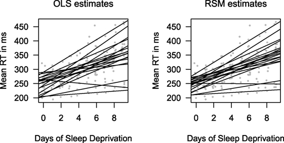
Figure 1. Estimates of individuals’ regression lines. The response times (RT) are in milliseconds (ms). The left panel shows the results using OLS to calculate separate coefficients for each student. The right panel uses a RSM model where information of other students is used to shrink the coefficient estimates. The values for Days (light gray dots) have had a small random jitter added to them to make them easier to see.

Much education research relies on measuring growth and there are several excellent textbooks for this (e.g., Plewis, 1985; Singer and Willett, 2003; Grimm et al., 2016). There is interest both in how student scores increase and decrease over the years and also how school statistics (e.g., attendance rates, graduation rates) fluctuate. Often teachers and policy makers want to know if the students’ and schools’ trajectories are in the right direction and if they are likely to reach certain thresholds (e.g., proficiency for students or government dictated targets for schools). With the increase in the use of accountability statistics in education for grading teachers and schools, and also outside of education (e.g., in health care (Foley and Goldstein, 2012)), the accuracy of these estimates are critical. While researchers in most laboratory research have much control over the number of repeated measurements, those conducting field research in education and the social sciences often do not have much control. The objective of the current research is to examine how many points are necessary per student/school to yield accurate slope estimates using the RSM model.

1. An Example: Graduation Rate Growth

In the US, states evaluate schools based on whether they have achieved or are making progress toward reaching several goals. One of these goals concerns the school’s graduation rate. For example, for the 2014–2015 school-grading cycle, New Mexico recorded each high school’s graduation rate for the previous 3 years² and awarded points for graduation rate growth. This was estimated (that year) using the slope estimates from a RSM.³ These values were used as part of the overall grade that was awarded to the school.

The conditional means for the intercepts and slopes are created using lme4 (Bates et al., 2015) with:

coef(lmer(rate ~ year + (year|school)))

and the OLS estimates with:

coef(lm(rate ~ 0 + as.factor(school)+ as.factor(school)*year))

Figure 2A shows that the estimates from the RSM and the OLS models are very different (r = 0.11). Note also that the spread of the slope estimates is very small for the RSM estimates, SD = 0.62, compared with the OLS estimates, SD = 10.16. Figure 2B shows that the slope estimates from the RSM method are closely associated with the intercept estimates (r = 0.99), though with a much smaller spread. The small SD and the correlation patterns are clear indicators that these estimates are problematic. Analysis of some of the individual school results also raised alarms. Consider two schools:

FIGURE 2

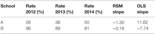
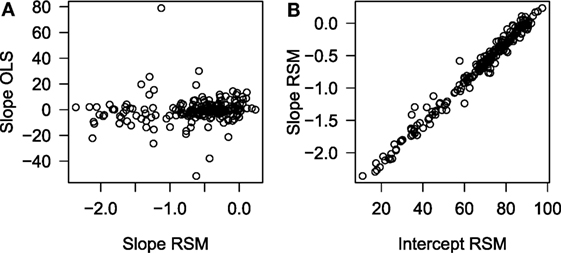
Figure 2. A scatter plot of the relationship between the conditional means for the intercept and for the slope. (A) Slope RSM and (B) intercept RSM.

While School A has a low graduation rate it is clearly increasing and the opposite is true for School B. However, the RSM method estimates that School A’s rate is decreasing and School B’s rate is near zero.

To determine how often data sets like these would produce problematic estimates 10,000 bootstrap samples of these data were taken and the correlation between slope estimates from the two methods recorded. Figure 3 shows the histogram of these correlations. There are two clear modes: one near zero and one near 0.85. Fifty-four percent are below r = 0.25 and only 27% are above r = 0.75 (which might be deemed high enough for some purposes). When problems like these were presented to Secretary of Education in New Mexico, the Public Education Department stopped using the RSM model to estimate the growth in graduation rates.

FIGURE 3

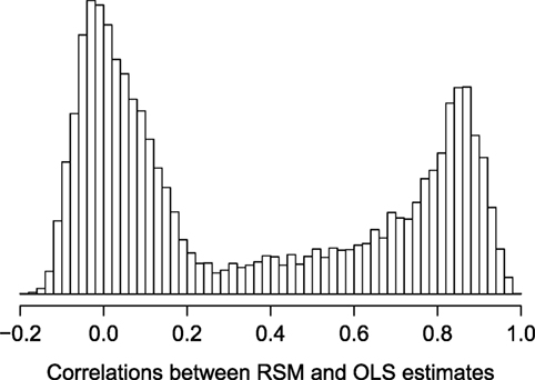
Figure 3. Histogram of the correlations from 10,000 bootstrap samples from the 2012 to 2014 graduation rates in New Mexico between the random slope multilevel and fixed slope (OLS) models.

2. Problem Description and Method

The example above shows that using RSM models can be problematic for data with similar characteristics to New Mexico graduation rate data. It is important to show when this procedure produces reliable and unreliable results. Two simulations will explore the limits of the random slope model for estimating growth. The key variable being manipulated is the number of years of data. The prediction is that the accuracy of the RSM (and OLS) estimates will increase with number of time points.

The language used to describe the simulations will assume that the analyst is attempting to measure student growth from a series of test scores. Suppose the goal is to measure student growth per year and that each student has a 0–100 percentile score on a standardized annual test for several consecutive years. Denote the ith student’s score in the jth year as score_ij and denote the number of years since the first year of data with year_ij = 0…10. An intuitive estimate of growth for any student would be the slope estimated from an OLS regression using only this student’s data. The model would be: score_i = β₀ + β₁year_i + e_i for each student. A single regression for the whole sample could be solved by estimating a separate ($\widehat{{\beta }_{0i}}$, $\widehat{{\beta }_{1i}}$) pair for each student by having n dummy variables and including their interactions with year_i. There would be two estimates for each student, one for the main effect and one for the interaction with year_ij. If there are n = 100 students, this would mean that there are 200 coefficients estimated.

Stein (1956) showed that if there are more than two individuals estimating statistics for individuals can be improved by using information from the other individuals. Efron and Morris (1977) describe this for a non-statistical audience. See Efron and Hastie (2016) (Chapter 7) for its place within modern statistics. Since Stein’s paper, several alternatives for shrunken estimates have been used. One alternative is to estimate the slopes based on the RSM model:

$score{s}_{ij}=({\beta }_0+u_{0j})+({\beta }_1+u_{1j})yea{r}_{ij}+e_{ij}$ (2)

This involves estimating just one ($\widehat{{\beta }_0}$, $\widehat{{\beta }_1}$) pair, the variances for the random variables u_0j and u_1j (it is usually assumed they are normally distributed with means of zero), and optionally their covariance. These values are used to estimate a slope for each student by calculating the conditional modes, which with the linear models considered here are also the conditional means. This can be done with many multilevel packages and are often called EM (empirical Bayesian) estimates or BLUPs (best linear unbiased predictions) in the literature for many statistics packages (e.g., Stata, see Rabe-Hesketh and Skrondal (1992)).

In this simulation the R package lme4 (Bates et al., 2015, version 1.1-12) is used. R is free and can be downloaded from https://cran.r-project.org/. The code to estimate the slopes using a RSM model, with the correlation between the random variables estimated, is:

estimates <- coef(lmer(scores ~ year + (year|students)))$students$year

The code where the correlation between the random slope and the random intercept is fixed at zero is:

estimates <- coef(lmer(scores ~ 1 + year + (1|students) + (0 + year|students))) $students$year

In this paper, the first of these is referred to as RSM 1 and the second RSM 2. Calculating individual coefficients (the following produces estimates for both β₀s and β₁s) separately for each student using OLS is done in R with:

estimates <- coef(lm(score ~ 0 + as.factor(student)*year + as.factor (student)))

3. Simulation 1: Linear Relations and Normal Distributions

Let there be 100 students with annual test scores for between 3 and 10 years of data. The sample size of one hundred students was chosen as the approximate number of students in a single grade in an average public school in the US. On average, there are more students in high schools and fewer in elementary schools.⁴ Each student has a true underlying value for their individual intercept and slope. These are drawn from Normal distributions, μ = 0, σ = 1 for the intercept; and μ = 0, σ = 0.2 for the slope, with the constraint that they are uncorrelated. The data will fan-out. This occurs with much educational data and is often called the Matthew effect (Walberg and Ling Tsai, 1983; Stanovich, 1986). The year variable is not being centered in the analyses. The residual terms are drawn from a Normal distribution with μ = 0 and σ = 1. If σ is smaller the estimates are more accurate and if σ is larger the estimates are less accurate. The distribution of data in real-world applications will depend on the standardized tests that are used and some are designed approximate these assumptions. The main R code to create the test score is:

score <- int + sl*year + rnorm(n*cormat[i,2],0,1)

where int and sl are variables for the true intercept and slope for each student, year is which year of data the score is for, and the part of the cormat matrix that is used above is the number of time points for the replication.

The complete code used for the simulations are in the Appendix. R (R Core Team, 2016, R version 3.3.2 (2016-10-31)) was used for the simulations. One thousand replication data sets for each of the 8 possible number of years of data (3–10) were created. RSM 1, RSM 2, and OLS were used to estimate the growth. The key part of the code is below, where CMs1 are the estimates from RSM1 (correlation between the variance terms estimated), CMs2 are from RSM2 (correlation set to zero), and OLS for ordinary least squares.

CMs1 <- as.matrix(coef(lmer(score~year + (year|student)))$student)

CMs2 <- as.matrix(coef(lmer(score~year +

 (1|student) + (0 + year|student))) $student)

OLS <- matrix(coef(lm(score ~ 0 + as.factor(student)*year +

 as.factor(student))),ncol = 2)

The as.matrix and matrix functions are so that the data are stored in a convenient manner for comparison.

Two statistics were used to evaluate these procedures. First, as the data were created in the same way for 1,000 runs, the SDs of the estimated slopes should be near the value used to create them. Second, these values were correlated with the true underlying growth (the sl variable from above, which is known because this is a simulation) used to create the data to produce a measure of the accuracy of the statistical procedure for each replication. Ideally $\widehat{{\beta }_1}s$ should be similar to β₁s, so a good procedure should have a high correlation. The entire code used to produce this paper, including simulations, tables, and figures, is available from the author as a knitr document (Xie, 2013).

4. Results

Figure 4 shows the histograms of the SDs of the slope estimates from each of the 1,000 replications for situations with 3 and 10 years of data, and for the three estimation methods. These data were created such that the SD of the underlying true slope was σ = 0.2. Starting with the top row (3 years of data), the two RSM methods have smaller SDs than the OLS method. This is expected because the individual students’ slope estimates are shrunk toward the center of that replication’s distribution. Examining the histogram for RSM 2, 26.6% of these are less than 0.0001 (i.e., very small and 17% are equal to zero within R’s level of precision). While the analyst should realize that there is an estimation problem if the estimates have a zero SD, there is a high proportion of non-zero, but small, SDs that might be more difficult to detect as aberrant. If these values are ranked or transformed into z-scores, then even minute differences near zero may appear large. As the number of years of data increase, there were fewer obviously problematic results. RSM 2 had: 7.6, 1.1, and 0.0% cases with SDs less than 0.0001 when there were 4, 5, and 6 years of data per student. The bottom row in Figure 4 shows the plots for when there are 10 years of data. The tendency is for the SDs of the RSM models to be slightly smaller than the true σ = 0.2 because of shrinkage and the OLS SDs to be slightly above σ = 0.2 because of sampling variability.

FIGURE 4

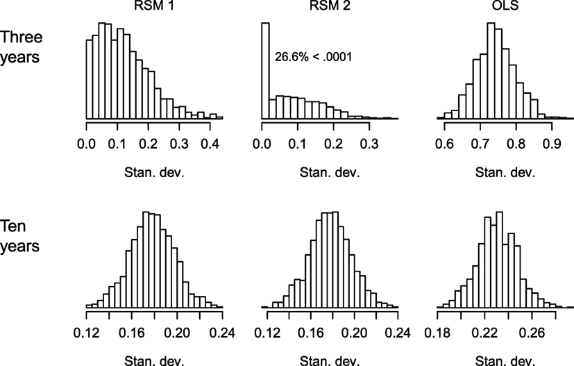
Figure 4. Histograms for the SD of the slope estimates for the different estimation methods when there are 3 and 10 years of data. Simulation 1 (normally distributed linear relationships). RSM 1 and RSM 2 refer to estimating the correlation between the random variables (1) and fixing it at zero (2).

The key question is whether the estimates accurately measure the true slope that was used to create the data for each student. Several measures can be used in simulation studies to identify whether a statistic tends to be accurate (Feinberg and Rubright, 2016). Here, there are two sets of continuous measures: the true growth values used to create the data and the estimated values. A simple measure of this is the Pearson correlation between the estimated and the true underlying slope. Figure 5 shows histograms for these correlations for the three methods when there are 3 and 10 years of data. When there are only 3 years of data (the top row), all the methods produced some correlations that were either negative or near zero. The zeroes in the top-middle panel correspond to cases where the SD was zero (to the level of R’s precision). The OLS method had fewer non-positive correlations. The bottom row shows that when many of the assumptions of these models are meet (linear relationships, normally distributed data) and there are ten measurements per student, all these methods performed relatively well.

FIGURE 5

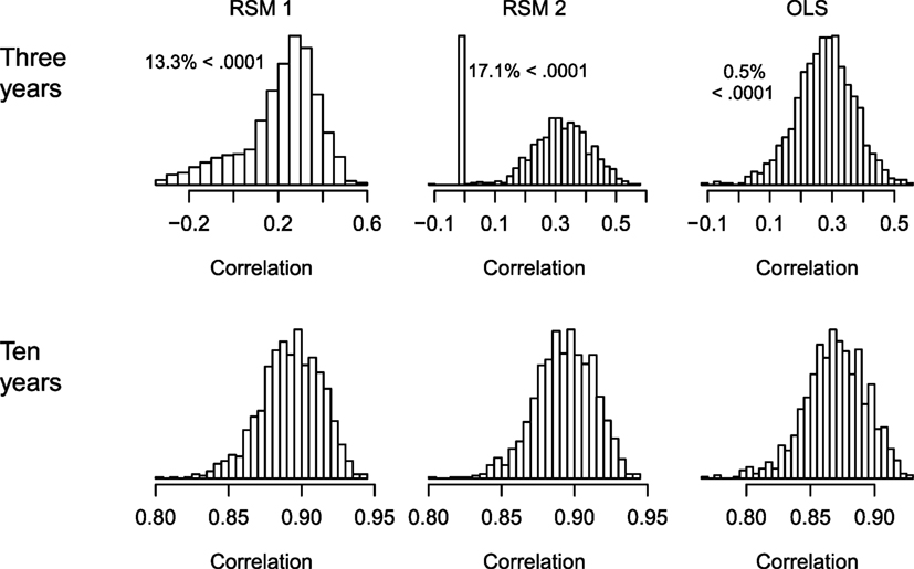
Figure 5. Histograms of the correlations between the estimated and true underlying slopes for the different estimation methods when there are 3 and 10 years of data. Simulation 1 (normally distributed linear relationships). RSM 1 and RSM 2 refer to estimating the correlation between the random variables (1) and fixing it at zero (2).

The central tendency and spread of these correlations when there are three time points are worth noting. The mean and median for each of the three methods are: mean = 0.21 and median = 0.25 for RSM 1; mean = 0.27 and median = 0.30 for RSM 2; and mean = 0.28 and median = 0.28 for OLS. The SD and inter-quartile range (IQR) for each of the three methods are: SD = 0.17 and IQR = 0.19 for RSM 1; SD = 0.15 and IQR = 0.17 for RSM 2; and SD = 0.09 and IQR = 0.12 for OLS.

Table 1 shows that the mean correlations increased for all three methods with the number of years of data per student. RSM 2 tended to have slightly higher correlations than RSM 1 (but if the correlation between u_0j and u_1j is increased close to 1, RSM 2 has slightly higher correlations). Table 2 shows the frequency of cases out of 1,000 replications that had correlations that were less than 0.0001 including negative correlations. These occurred mostly when there were only three or four time points and more frequently for the RSM methods.

TABLE 1

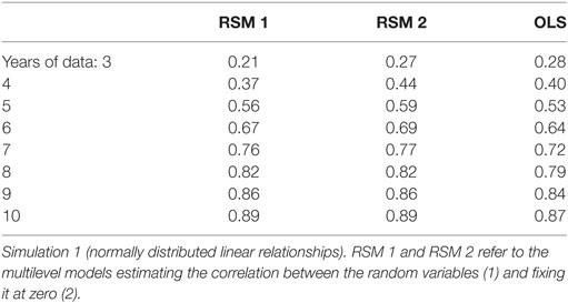
Table 1. The mean correlations between the estimated slope and the true underlying slope.

TABLE 2

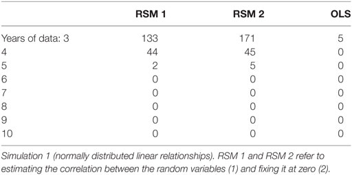
Table 2. The number of correlations, out of 1,000, that were less than 0.0001 (including negative values) for between the estimated slope and the true underlying slope.

5. Discussion

There two main conclusions. First, basing the estimation of the two values that determine a line on just three points should be done cautiously if the points are measured with error. This was shown with the OLS estimates having high SDs. The hope by many using multilevel methods is that by “borrowing strength” from the data of other students, the estimates become more accurate. While the basic descriptive statistics of the correlations support this when there are several time points, examining the distributions in Figure 5 highlight the second statistical conclusion: “multilevel models are tools to be used with care and understanding” (Goldstein, 2003, p. 12). These are complex models and unreliable results can emerge when they are pushed beyond their limits. The distributions in the top row show that these methods’ limits have been passed. When there are only three time points, the estimates can be unreliable.

Analysts should not restrict themselves to only one method. If, for example, an analyst used a RSM model with just a few time points per students, a student’s slope based just on these scores (OLS) may be positive, but the RSM estimates may be negative. If students have access to their scores they can calculate their own OLS scores. This will lead to some dispute and undermine the credibility of the analysis. However, the analyst could use a RSM method and an OLS method to identify situations where the estimates diverge. When cases with odd patterns emerge, like those shown in the example, the analyst could use the OLS estimates because, although they may be more variable, they are less likely to produce highly irregular estimates (Table 2).

The main recommendation from this section is to have as many time points as is feasible. When there were only three or four points, the accuracy was low. In some situations, it is not possible to have more points. For example, if trying to estimate growth of third graders, there may not be four previous scores from reliable standardized tests. There is already concern among many parents about the amount of time allocated to these tests. If an adequate number of tests are not available estimating growth may be unwise. Often no estimate is better than an unreliable one. It is worth stressing that using more reliable measures (e.g., longer tests, using paradata like response latencies to improve estimates, Wright (2016)) can also improve the growth estimates. However, this is not always possible. For example, consider the example of school graduation rates. These are annual statistics. While some improvements can be made in making reports of these more accurate and comparable across institutions, random variability will remain.

The situations examined in this section involved creating data with normal distributions and linear relationships. These aspects of the data are often assumed by analysts in statistical models, but they are rare in nature (Micceri, 1989). In the next section, data that are not normally distributed are examined.

6. Simulation 2: Negatively Skewed Distribution

While test score data can be constructed to be normally distributed, much of the data both in education and elsewhere are not normally distributed (Micceri, 1989). Several steps were followed to create negatively skewed data for the simulation presented in this section. First, values were drawn from a normal distribution with a mean based on the linear function used in the previous section, (x_ij = β₀ + u_0j) + β₁ + u_1j)year_ij. β₀ and β₁ were drawn from normal distributions as above. The x_ij values were then squared. The negative of this value was used in the logistic distribution function in R (plogis). This was multiplied by 80 and subtracted from 80. A number, randomly drawn from a uniform distribution from 0 to 20, was added to it. This creates scores from 0 to 100 that are negatively skewed, approximately −0.5. This distribution was used to approximate scores from school tests that often use a 0–100 scale where above 90 is an A, above 80 is a B, etc., and with most student scores in the D–A range. The R code is:

score <- 80 - (80*plogis(rnorm (n,-1*(B0 + year*B1)))ˆ2) + runif(n,0,20)

The scores were kept as continuous values. Additional simulations were conducted varying other aspects of the data, including using discrete values (accuracy decreased slightly) and allowing u_0j and u_1j to be correlated (negative correlations decreased accuracy, positive correlations increased accuracy), but are not reported here to focus on the distribution alteration, which had a larger effect than these. Other than how the data were created, this simulation was identical to the first.

7. Results and Discussion

As with Simulation 1, the SD of the estimates and their correlations with the true values are used to evaluate the procedures. However, because of the way in which the data were created the expected value of estimated slope from the linear models is not, even under ideal circumstances, expected to be the β₁ used to create the data. Therefore, the size of the SDs of the estimates will be different than in Simulation 1. Furthermore, the relationship between the estimated and actual growth is not expected to be linear. The results using Spearman’s ρ correlation were analyzed and very similar to those reported below using Pearson’s correlation.

Figure 6 shows the histograms of the SDs of the estimated slopes from each replication for situations with 3 and 10 years of data, and for the three estimation methods. The results have a similar pattern to those reported for Simulation 1. Starting with the top row (3 years of data), the two RSM methods have smaller SDs than the OLS method. For RSM 2, where the correlation between the random variables is fixed at zero, 35.6% of these are less than 0.0001. This is about 50% more than reported for Simulation 1 with normally distributed data. There were: 14.6, 2.4, and 0.1% (1 of 1,000 replications), cases with SDs less than 0.0001 when there were 4, 5, and 6 years of data per student, respectively. The bottom row in Figure 6 shows the plots for when there are 10 years of data. The tendency is for the SDs of the RSM models to be smaller than the OLS SDs.

FIGURE 6

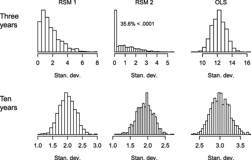
Figure 6. Histograms of the SDs of the slope estimates for the different estimation methods when there are 3 and 10 years of data. Simulation 2 (negatively skewed). RSM 1 and RSM 2 refer to estimating the correlation between the random variables (1) and fixing it at zero (2).

Figure 7 shows histograms for these correlations for the three methods when there are 3 and 10 years of data. When there are only 3 years of data (the top row), all the methods produce some correlations that are either negative or zero, though there are very few of these for the OLS method. As with Simulation 1, the spike in the top-middle panel at r = 0 corresponds with cases where the SD was effectively zero. The mean and median for each of the three methods when there are only three time points were: mean = 0.15 and median = 0.20 for RSM 1; mean = 0.23 and median = 0.26 for RSM 2; and mean = 0.23 and median = 0.24 for OLS. The SD and inter-quartile range (IQR) for each of the three methods were: SD = 0.18 and IQR = 0.23 for RSM 1; SD = 0.14 and IQR = 0.18 for RSM 2; and SD = 0.09 and IQR = 0.12 for OLS. The bottom row shows that these models preformed much better when there were ten measurements per student.

FIGURE 7

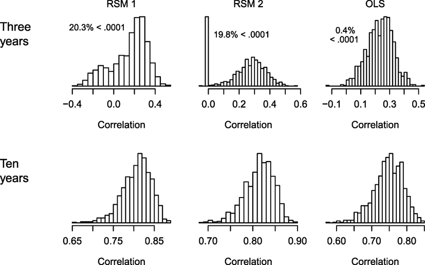
Figure 7. Histograms of the correlations between the estimated and true underlying slopes for the different estimation methods when there are 3 and 10 years of data. Simulation 2 (negatively skewed). RSM 1 and RSM 2 refer to estimating the correlation between the random variables (1) and fixing it at zero (2).

Table 3 shows that the means of the correlations increased for all three methods as the number of years of data per student increased. When there were at least five time points, the RSM methods had higher mean correlations than the OLS method. Table 4 shows the frequency of cases out of 1,000 replications that had correlations that were less than 0.0001 including negative correlations. These occurred mostly when there are only three or four time points and more frequently for the RSM methods. There were more of these aberrant cases here than there were reported for Simulation 1.

TABLE 3

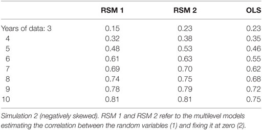
Table 3. The mean correlations between the estimated slope and the true underlying slope.

TABLE 4

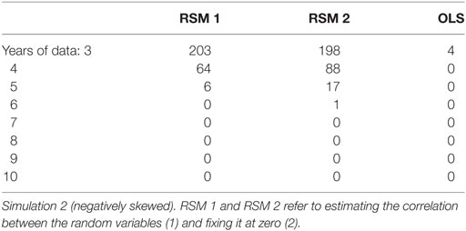
Table 4. The number of correlations, out of 1,000, that were less than 0.0001 (including negative values) for between the estimated slope and the true underlying slope.

The main conclusion for the skewed data evaluated in this study is that the results are likely to be even less accurate than with normally distributed data. Education data can be very messy. There are often missing values, outliers, and non-independence (i.e., clustering). What is striking in the results reported here and even without a lot of these factors the RSM procedures still performed poorly when there were less than six time points.

8. General Discussion

Estimating growth from only a few points will often produce poor estimates. It is intuitive that if the individual scores are measured with error that the slope of three or four points may not be reliable. This is one reason why random slope models seem attractive: information from other individuals’ scores can be “borrowed” to improve reliability. Information of other students’ performance is used to inform individual slope estimates. However, when there are not many time points these complex models can produce results that are aberrant. These include cases where the estimated growth is negatively correlated with the true underlying growth. Results from individual cases, like Schools A and B in the example, can undermine the credibility of the accounting system. Thus, the main conclusion is:

---

The RSM can be unreliable with less than six time points and are particularly like to be poor with three or four time points.

---

These results reinforce the recommendation to have as many points as possible. In many laboratory studies, the researcher can add additional time points. For example, Belenky et al. (2003) could have taken multiple measurements each day. This is not always possible in education. There is significant backlash against the number of standardized tests that students are already taking. It might not be practical and would likely be politically unpopular to include more tests within each year. For older students, there might be several years of annual test score data, but the interest may be just in recent growth. The same issues apply to schools.

Policy makers can pressure analysts to produce estimates even when the analyst is aware that the estimates may be unreliable. This is one of the reasons why it is important to report the error associated with any statistics that are reported (Wilkinson and the Task Force on Statistical Inference, 1999; Wright, 2003). Bootstrap methods can be used to examine whether slight variations in the data produce very different results. As shown with the example, these estimates can be quite variable. For the particular problem of measuring growth, the RSM methods did do better than the OLS method, providing that there were enough time points. However, in both reported simulations, the RSM methods produced results that were often negatively correlated with the true slope. When this happens, individuals could have increasing scores but a negative growth estimate, as shown with the graduation rate growth example. Reporting that a student or school has a negative growth estimate from a complex model when the student or principal can see that their scores have increased (as would be found using OLS of just that student’s scores) will create disputes. Estimating these growth scores with different methods may help to identify these cases and allow them to be adjusted. The OLS estimates could be used when the two methods produce very different results. Although the OLS estimates have a larger variation than the RSM estimates, they do not produce as many estimates that are negatively correlated with the true slope and do not produce estimates that will be clearly at odds with an individual student’s or school’s data as with the example for Schools A and B above. The poor estimates for Schools A and B harm the public’s confidence in the accountability system.

The focus of this paper was on the relationship between the number of time points and the slope estimates. Other aspects, like missing values and the variability of the individual scores, should be considered in future research. Researchers are welcome to adapt the code that appears in the Appendix. The RSM procedure was shown, in both example and simulations, to be problematic. There is no recommended ideal procedure that will always work. Even if using seemingly magic phrases like “analytics,” “deep learning,” and “value-added modeling” (Braun, 2013), often the data do not provide sufficient information to yield accurate estimates. If you only have a small number of time points, each measured with error, then the estimates of the slope with any procedure can be poor. However, the RSM procedures will occasionally produces very bad estimates.

9. Recommendations

The following are of importance.

1. Use as many time points as is feasible. The reliability of the slope estimates will increase with the reliability of the data themselves, but from these simulations having at least six time points seems appropriate for most education data sets.

2. If the RSM methods produce small SDs or produce estimates that are very different from the OLS estimates, the RSM method is likely to be unreliable. The OLS slope estimates are preferred in this case and should be used. This will more likely occur when there are less than six time points than when there are more and can occur often when there are only three time points (e.g., the New Mexico graduation rate data).

3. With any complex statistical model, it can be worth estimating the model multiple times for bootstrap samples to observe if the estimates are reliable.

4. The OLS procedure is simpler to explain. If transparency is important for the accountability system, this would be another argument for not using RSM. The OLS estimates can also be calculated with the individual student’s or school’s own data.

Author Contributions

All aspects of the research were conducted by DW.

Conflict of Interest Statement

The author declares that the research was conducted in the absence of any commercial or financial relationships that could be construed as a potential conflict of interest.

Footnotes

1. ^http://www.bristol.ac.uk/cmm/learning/mmsoftware/.
2. ^School data for several years are at http://aae.ped.state.nm.us/ accessed September 20, 2017.
3. ^There were a few new schools that had only a single graduation rate. If a school has only 1 year of data the RSM will still estimate its growth by borrowing information from other schools. The OLS method will not.
4. ^https://nces.ed.gov/programs/digest/d15/tables/dt15_216.20.asp, accessed May 31, 2017.

References

Bates, D., Mächler, M., Bolker, B., and Walker, S. (2015). Fitting linear mixed-effects models using lme4. J. Stat. Softw. 67, 1–48. doi: 10.18637/jss.v067.i01

CrossRef Full Text | Google Scholar

Belenky, G., Wesensten, N. J., Thorne, D. R., Thomas, M. L., Sing, H. C., Redmond, D. P., et al. (2003). Patterns of performance degradation and restoration during sleep restriction and subsequent recovery: a sleep dose-response study. J. Sleep Res. 12, 1–12. doi:10.1046/j.1365-2869.2003.00337.x

PubMed Abstract | CrossRef Full Text | Google Scholar

Braun, H. I. (2013). Value-added modeling and the power of magical thinking. Eval. Pub. Pol. Educ. 21, 115–130. doi:10.1590/S0104-40362013000100007

CrossRef Full Text | Google Scholar

Efron, B., and Hastie, T. (2016). Computer Age Statistical Inference: Algorithms, Evidence, and Data Science. New York: Cambridge University Press.

Google Scholar

Efron, B., and Morris, C. (1977). Stein’s paradox in statistics. Sci. Am. 236, 119–127. doi:10.1038/scientificamerican0577-119

CrossRef Full Text | Google Scholar

Feinberg, R. A., and Rubright, J. D. (2016). Conducting simulation studies in psychometrics. Educ. Measure. 35, 36–49. doi:10.1111/emip.12111

CrossRef Full Text | Google Scholar

Foley, B., and Goldstein, H. (2012). Measuring Success: League Tables in the Public Sector. London: British Academy.

Google Scholar

Goldstein, H. (2003). Multilevel Statistical Models, 3 Edn. London, UK: Arnold.

Google Scholar

Grimm, K. J., Ram, N., and Estabrook, R. (2016). Growth Modeling: Structural Equation and Multilevel Modeling Approaches. New York: Guilford Press.

Google Scholar

Laird, N. M., and Ware, J. H. (1982). Random-effects models for longitudinal data. Biometrics 38, 963–974. doi:10.2307/2529876

PubMed Abstract | CrossRef Full Text | Google Scholar

Micceri, T. (1989). The unicorn, the normal curve, and other improbable creatures. Psychol. Bull. 105, 156–166. doi:10.1037/0033-2909.105.1.156

CrossRef Full Text | Google Scholar

Muthén, B. (1997). “Latent variable growth modeling with multilevel data,” in Latent Variable Modeling & Applications to Causality, ed. M. Barkane (Cambrdige, MA: Springer-Verlag), 149–161.

Google Scholar

Plewis, I. (1985). Analysing Change: Methods for the Measurement and Explanation of Change in the Social Sciences. West Sussex, UK: Wiley.

Google Scholar

Preacher, K. J., Wichman, A. L., MacCallum, R. C., and Briggs, N. E. (2008). Latent Growth Curve Modeling. Thousand Oaks, CA: SAGE.

Google Scholar

R Core Team. (2016). R: A Language and Environment for Statistical Computing. Vienna, Austria: R Foundation for Statistical Computing.

Google Scholar

Rabe-Hesketh, S., and Skrondal, A. (1992). Multilevel and Longitudinal Modeling Using Stata, 2nd Edn, Vol. 1–2. College Station, TX: Stata Press.

Google Scholar

Rosseel, Y. (2012). lavaan: an R package for structural equation modeling. J. Stat. Softw. 48, 1–36. doi:10.18637/jss.v048.i02

CrossRef Full Text | Google Scholar

Singer, J. D., and Willett, J. B. (2003). Applied Longitudinal Data Analysis: Modeling Change and Event Occurrence. New York: Oxford University Press.

Google Scholar

Stanovich, K. E. (1986). Matthew effects in reading: some consequences of individual differences in the acquisition of literacy. Read. Res. Q. 21, 360–407. doi:10.1598/RRQ.21.4.1

CrossRef Full Text | Google Scholar

Steele, F. (2008). Multilevel models for longitudinal data. J. R. Stat. Soc. A 171, 5–19. doi:10.1111/j.1467-985X.2007.00509.x

CrossRef Full Text | Google Scholar

Stein, C. (1956). “Inadmissibility of the usual estimator for the mean of a multivariate normal distribution,” in Proceedings of the Third Berkeley Symposium on Mathematical Statistics and Probability, 1954–1955 (Berkeley: University California Press), 197–206.

Google Scholar

Walberg, H. J., and Ling Tsai, S. (1983). Matthew effects in education. Am. Educ. Res. J. 20, 359–373. doi:10.2307/1162605

CrossRef Full Text | Google Scholar

Wilkinson, L., and The Task Force on Statistical Inference. (1999). Statistical methods in psychology journals: guidelines and explanations. Am. Psychol. 54, 594–604. doi:10.1037/0003-066X.54.8.594

CrossRef Full Text | Google Scholar

Wright, D. B. (2003). Making friends with your data: improving how statistics are conducted and reported. Br. J. Educ. Psychol. 73, 123–136. doi:10.1348/000709903762869950

PubMed Abstract | CrossRef Full Text | Google Scholar

Wright, D. B. (2016). Treating all rapid responses as errors (TARRE) improves estimates of ability (slightly). Psychol. Test Assess. Model. 58, 15–31.

Google Scholar

Wright, D. B., and London, K. (2009). Multilevel modelling: beyond the basic applications. Br. J. Math. Stat. Psychol. 62, 439–456. doi:10.1348/000711008X327632

PubMed Abstract | CrossRef Full Text | Google Scholar

Xie, Y. (2013). Dynamic Documents with R and Knitr. Boca Raton, FL: Chapman and Hall/CRC.

Google Scholar

Appendix

The R code for the first simulation, with normally distributed data. The function for creating correlated values (other simulations available from the author used non-zero values) is from http://stats.stackexchange.com/questions/38856/how-to-generate-correlated-random-numbers-given-means-variances-and-degree-of.

correlatedValue = function(x, r){

 r2 = r**2; ve = 1-r2; SD = sqrt(ve)

 e = rnorm(length(x), mean=0, sd = SD)

 y = r*x + e; return(y)}

set.seed(8374)

n <- 100

runs <- 8*1000

cormat <- matrix(nrow=runs,ncol = 38)

cormat [,1:2] <- c(1:runs, rep (3:10, runs/8))

options(warn=-1)

for (i in 1:runs){

 if (i %%100 == 0) message(i) #to track progress

 student <- rep (1:n, each = cormat[i,2])

 int <- rep(ival <- rnorm(n,0,1),each=cormat[i,2])

 sl <- rep(sval <- correlatedValue(ival,0.0)/5,each=cormat[i,2])

 year <- rep (0:(cormat[i, 2]-1),n)

 score <- int + sl*year + rnorm(n*cormat[i, 2], 0, 1)

 CMs1 <- as.matrix(coef(lmer(score~year + (year|student)))$student)

 CMs2 <- as.matrix(coef(lmer(score~year + (1|student) + (0 + year|student)))$student)

 OLS <- matrix(coef(lm(score ~

 0 + as.factor(student)*year + as.factor(student))),ncol = 2)

 vals <- cbind(CMs1,CMs2,OLS,ival,sval)

 cormat[i,3:30] <- cor(vals)[lower.tri(cor(vals))]

 cormat[i,31:38] <- apply(vals[,1:8],2,sd)}

 options(warn = 0)

cormat[is.na(cormat)] <- 0 #This noted in results

cormat <- as.data.frame (cormat)

names(cormat) <- c("runs","grades",

  "CI1S1","CI1I2","CI1S2","CI1OI","CI1OS","CI1i","CI1s",

            "CS1I2","CS1S2","CS1OI","CS1OS","CS1i","CS1s",

              "CI2S2","CI2OI","CI2OS","CI2i","CI2s",

                "CS2OI","CS2OS","CS2i","CS2s",

                         "COIOS","COIi","COIs",

                                  "COSi","COSs",

                                       "Cis",

"sdI1","sdS1","sdI2","sdS2","sdOI","sdOS","sdi","sds")

cormat1 <- cormat

The code for the second simulation is:

correlatedValue = function(x, r){

 r2 = r**2; ve = 1-r2; SD = sqrt(ve)

 e = rnorm(length(x), mean=0, sd=SD)

 y = r*x + e; return(y)}

set.seed(83214)

n <- 100

runs <- 8*1000

cormat2 <- matrix(nrow=runs,ncol=38)

cormat2[,1:2] <- c(1:runs,rep(3:10,runs/8))

options(warn=-1)

for (i in 1:runs){

 if(i %%100 == 0) message(i)

 student <- rep(1:n,each=cormat2[i,2])

 int <- rep(ival <- rnorm(n,0,1),each=cormat2[i,2])

 sl <- rep(sval <- correlatedValue(ival,0)/5,each=cormat2[i,2])

 year <- rep(0:(cormat2[i,2]-1),n)

 score <- 80-(80*plogis(rnorm(n*cormat2[i,2],-1*(int + year*sl)))ˆ2) + runif(n*cormat2[i,2],0,20)

 CMs1 <- as.matrix(coef(lmer(score~year + (year|student)))$student)

 CMs2 <- as.matrix(coef(lmer(score~year + (1|student) + (0 + year|student)))$student)

 OLS <- matrix(coef(lm(score~0 + as.factor(student)*year + as.factor(student))),ncol = 2)

 vals <- cbind(CMs1,CMs2,OLS,ival,sval)

 cormat2[i,3:30] < − cor(vals)[lower.tri(cor(vals))]

 cormat2[i,31:38] < − apply(vals[,1:8],2,sd)}

 options(warn = 0)

cormat2[is.na(cormat2)] < − 0 # Reported in results

cormat2 <- as.data.frame(cormat2)

names(cormat2) < − c("runs","grades",

  "CI1S1","CI1I2","CI1S2","CI1OI","CI1OS","CI1i","CI1s",

            "CS1I2","CS1S2","CS1OI","CS1OS","CS1i","CS1s",

              "CI2S2","CI2OI","CI2OS","CI2i","CI2s",

                "CS2OI","CS2OS","CS2i","CS2s",

                         "COIOS","COIi","COIs",

                                  "COSi","COSs",

                                       "Cis",

"sdI1","sdS1","sdI2","sdS2","sdOI","sdOS","sdi","sds")