Assessment of Thermal Maturity Trends in Devonian–Mississippian Source Rocks Using Raman Spectroscopy: Limitations of Peak-Fitting Method

Introduction

Several factors contribute to the generation of hydrocarbons in potential source rocks including the amount and type of organic material and temperature integrated over time (Hunt, 1979). This study focuses on one aspect: the assessment of thermal maturity which is defined as the extent to which temperature has affected organic matter during a rock’s geologic history (Dow, 1977; Taylor et al., 1998; Suárez-Ruiz et al., 2012). Temperature is an imperative attribute as it is the main kinetic control influencing the onset of hydrocarbon generation, and, depending on the type of organic material, progressively higher temperatures influence when oil and wet and dry gas are generated (Dow, 1977; Taylor et al., 1998; Suárez-Ruiz et al., 2012). Accurate assessment of source rock thermal maturity is therefore critical in petroleum systems analysis. This study focuses on the use of Raman spectroscopy as a tool to evaluating correlations generated between Raman spectral data and thermal maturity. The samples evaluated in this study (Table 1) originated from the Upper Devonian Ohio Shale and Lower Mississippian Sunbury Shale, both of which are potential source rocks to hydrocarbons produced in the study area (Cole et al., 1987).

TABLE 1

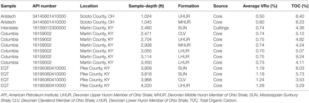
Table 1. Sample locations and lithology information.

Source rock thermal maturity is often evaluated using programmed pyrolysis and/or an optical technique termed vitrinite reflectance (VRo) (Mukhopadhyay, 1994; ASTM, 2015). During burial, the source rock experiences progressively higher temperature that results in the formation and coalescence of aromatic rings of carbon in vitrinite (Carr and Williamson, 1990). These rings form sheets which change the physical property of vitrinite reflectance, causing more light to be reflected. VRo requires that samples exhibit a high quality polish to insure vitrinite is scratch and relief free (Mukhopadhyay, 1994). This approach to quantifying the thermal maturity of shale has fundamental limitations as this technique is time-intensive and requires an experienced petrographer to interpret different types of kerogen such that only vitrinite is measured. This can be a difficult undertaking due to low concentrations of kerogen, presence of other types of organic matter (such as solid bitumen, which is not a kerogen) that have similar optical properties, vitrinite reflectance suppression, and the physical quality of the sample and its preparation (Lo, 1993; Mukhopadhyay, 1994; Lo and Cardott, 1995). Finally, interlaboratory studies to evaluate the reproducibility of VRo measurements suggested use of a common methodology improved measurement accuracy but that significant improvements were still required (Hackley et al., 2015).

As part of an evaluation of the petroleum resources of the Berea Formation, potential source rock samples were collected along a north to south transect with progressively greater burial depth provided an opportunity to collect and analyze samples with up-dip shallow to down-dip deeper position (Berea Consortium Release, 2017). Along this north to south transect, thermal maturity increases (Repetski et al., 2008; East et al., 2012). Because of disagreements between measured VRo values and hydrocarbon-type production, the measured sample-depth was also employed as a relative metric of thermal maturity, and, therefore, a property used in developing correlations with Raman spectroscopy. It should be noted that this rationale is not without its own limitations, as thermal maturity as a function of sample-depth is dependent on thermal gradient, which can vary through time, subsidence rate, uplift (or lack thereof), and faulting. Sample-depth was also used as a thermal maturity proxy by Schito et al. (2017).

Vibrational spectroscopy has been evaluated as a potential technique for predicting the thermal maturity of carbonaceous samples (Spotl et al., 1998; Ferrari and Robertson, 2000; Beyssac et al., 2002; Quirico et al., 2005; Rahl et al., 2005; Guedes et al., 2010, 2012; Hinrichs et al., 2014; Wilkins et al., 2014; Zhou et al., 2014; Chen et al., 2015; Bonoldi et al., 2016; Lünsdorf, 2016; Lünsdorf and Lünsdorf, 2016; Sauerer et al., 2017; Schito et al., 2017; Schmidt et al., 2017). Most of this research has focused on Raman spectroscopy, an analytical tool that provides fast, non-destructive analyses, requires little-to-no sample preparation, and can grant both qualitative and quantitative information about the analyte. Raman spectroscopy measures the amount of laser light scattered from a molecule when excited. Approximately one in one million photons is inelastically scattered with a shift in energy from the excitation wavelength (Smith and Dent, 2005). The magnitude of the shift is a function of the specific bonds in a molecule. Scattered light radiates in all directions and is collected using sophisticated optics, such that fingerprints of molecular vibrations are assessed. Selection rules for Raman spectroscopy require changes in a molecule’s polarizability as opposed to the change in dipole required by infrared (IR) spectroscopy (McCreery, 2000; Smith and Dent, 2005). Therefore, Raman spectroscopy is well suited for evaluating the C-C and C = C bonds contained in carbonaceous samples like shale. Raman spectra of shale reveal two characteristic peaks: the disordered, D- or D1-band, and the graphitic, or G-band (Wang et al., 1990). These features arise near ~1,310–1,370 and ~1,580–1,610 cm⁻¹, respectively; however, the exact frequency is dependent on the sample and the spectral acquisition parameters (Wang et al., 1990; Spotl et al., 1998; Matthews et al., 1999; Castiglioni et al., 2001; Beyssac et al., 2002; Quirico et al., 2005; Guedes et al., 2012; Lünsdorf et al., 2014; Li et al., 2015; Lünsdorf, 2016). Other D-vibrational modes have been characterized and are referred to as D2 (~1,620 cm⁻¹), D3 (~1,500 cm⁻¹), and D4 (~1,250 cm⁻¹). Again, these vibrational modes depend on the sample. While several studies have investigated the origin of the D-band (Wang et al., 1990; Matthews et al., 1999; Castiglioni et al., 2001), the G-band has been unambiguously assigned to aromatic ring breathing modes.

While studies comparing Raman spectral parameters to intrinsic properties like thermal maturity have uncovered some basic trends, they have employed a multitude of different experimental and spectral processing techniques to develop the correlations (Spotl et al., 1998; Quirico et al., 2003, 2005; Rahl et al., 2005; Guedes et al., 2010, 2012; Hinrichs et al., 2014; Lünsdorf et al., 2014; Wilkins et al., 2014; Zhou et al., 2014; Bonoldi et al., 2016; Lünsdorf, 2016; Lünsdorf and Lünsdorf, 2016; Schito et al., 2017). These methods differed in the number of samples evaluated, the acquisition parameters used to generate the data (excitation wavelength, spectral resolution, acquisition time, number of unique and random points measured per sample), data processing (i.e., baseline correction) and peak-fitting metrics (number of peaks, wavenumber, maximum peak width). Often, integral parameters such as the calculated spectral resolution of the Raman spectrometer were excluded from the experimental details, thereby challenging one’s ability to reproduce the proposed method.

A few studies in the literature have investigated some of the subjective variables that can have deleterious effects on correlations between Raman spectra and intrinsic sample properties. Quirico et al. (2005) evaluated 11 coal samples to identify limitations that exist for applying Raman spectroscopy to the thermal maturity of coal. Parameters such as laser wavelength and sample thermal stability with acquisition time were assessed. Also discussed were the challenges of selecting peak-fitting morphologies (Gaussian, Lorentzian, etc.) to adequately represent peaks obscured by other vibrational modes, such as those ancillary bands flanking the D-mode. This spectral region has been hypothesized by the authors to contain a “continuum” of vibrational modes, thereby limiting the use of the peak-fitting approach altogether. Although the reproducibility was limited, correlations were developed between VRo and D-FWHM (VRo = 3–7%), the intensity ratio of D/G (VRo = 3–7%), and G-FWHM (VRo = 1–3%). In general, the authors found that samples must have a VRo > 1% for accurate linear regressions. Several studies have evaluated samples with VRo < 1%, with some results showing reasonable correlations, and others exhibiting higher error with decreases in VRo% (Keleman and Fang, 2001; Hinrichs et al., 2014; Wilkins et al., 2014; Bonoldi et al., 2016; Lünsdorf, 2016; Schito et al., 2017). Correlations of Raman spectral parameters with VRo values ranging from 0.3 to 1.5% provided coefficients of determination (R²) of >0.90 when fit with power equations (Schito et al., 2017). Lünsdorf (2016) evaluated coal samples with VRo values as low as 0.50%. The development of linear correlations between Raman parameters and samples with VRo < 1.5% was challenged by sample fluorescence. Wilkins et al. (2014) also evaluated coal samples with measured VRo values ranging from 0.4 to 1.2%. The authors used multiple linear regression (MLR) to develop a model that showed good correlation and accuracy (R² = 0.89) when applied to samples dedicated for validating the MLR model. Bonoldi et al. (2016) evaluated both Raman and IR spectroscopy to compare the two techniques for developing thermal maturity relationships between Raman or IR parameters and samples having VRo values between 0.2 and 2.7%. While the sensitivity of the method decreased when the VRo < 1.0%, the study found that IR seemed better suited for analyzing low maturity samples. Interestingly, the G–D-band separation metric extended to the full 0.2–2.7% maturity range. Factors that could bias the correlations generated from peak-fitting the Raman spectra of carbonaceous samples were assessed and included baseline-correction technique, the curve fitting strategy (type of function, peak start position, position, and slope of baseline), intrinsic sample characteristics, the instrumental configuration, and operator interpretation (Lünsdorf et al., 2014). A linear baseline subtraction exhibited lower relative SDs for several samples, when contrasted to polynomial baseline-correction. The significance of the bias from operator interpretation led to the generation of a novel, automated peak-fitting algorithm (Lünsdorf, 2016).

This research not only explored the development of an accurate, robust Raman method to quantify thermal maturity trends in shale using both the measured VRo and sample-depth but also evaluated the suitability of the peak-fitting method altogether. The Raman spectra of 13 different shale samples were analyzed using different peak-fitting methodologies (number of peaks and maximum peak width) to gage how altering just one of these user-defined parameters would affect the correlation to thermal maturity. Given that Raman spectroscopy does not require tedious sample preparations, all Raman measurements were acquired on the bulk sample, irrespective of topography. This method was implemented with the motivation of potential field-portable applications, such that extensions of Raman spectroscopy to the well-site might be possible. Sauerer et al. (2017) employed a similar approach with the same field-portability possibilities in mind.

Materials and Methods

Samples and Sample Preparation

The 13 shale samples, extracted from four wells, were part of a larger sampling program (12 wells) used to assess thermal maturity in the Berea Consortium study (Berea Consortium Release, 2017). Along this north to south transect burial depth increases as does thermal maturity based on previous thermal maturity studies (East et al., 2012; Hackley et al., 2013; Araujo et al., 2014; Berea Consortium Release, 2017; Schmidt et al., 2017). Table 1 provides well and lithology information for the samples used in this study, which range from 1,024 to 4,220 ft in depth, and 0.5 to 1.29 VRo%. Table S1 in Supplementary Material provides the minimum and maximum VRo values for each sample.

Most of the samples came from core as they provided the greatest confidence in sample-depth and the fewest issues with contamination; however, one sample came from well cuttings in order to fill spatial gaps (Table 1). Gamma ray and density logs from individual wells were evaluated, and the former was used to select dark, organic-rich intervals (high gamma ray response) for analysis. Samples were received by RJ Lee Group, Inc. in powder-form and were applied by spatula to aluminum-coated borosilicate glass microscope slides. Loosely bound shale was removed using canned air such that (a) the remaining physisorbed particles were strongly adhered to the slide via electrostatic interactions, and (b) a monolayer was distributed to facilitate the analysis of different shale particles to better represent the bulk sample. The presence of a monolayer of shale particles was determined optically using bright-field microscope images. The typical sizes of the shale particles measured for this study ranged from a few micrometers to approximately 10–20 µm (<500 mesh, US). Measuring particles larger than this size was avoided due to the tendency to overlap with other particles.

Raman Instrumentation and Spectral Acquisition

This study was conducted using a Horiba LabRam HR800 Raman spectrometer (Horiba Scientific, Edison, NJ, USA), equipped with 473 nm excitation wavelength and a 600 grooves/mm grating. The spectral resolution of this configuration was 2.4 cm⁻¹. The spectrometer was calibrated using the 520.70 cm⁻¹ peak of a silicon wafer. A neutral density filter was employed such that 1% of the maximum laser power, or ~3.9 μW, interacted with the sample through a 100x long-working distance microscope objective (numerical aperture = 0.8), enabling the laser spot to be finely focused (~640 nm), such that individual shale particles could be measured. It should be noted that use of 633 and 784 nm excitation wavelengths were also evaluated, but did not reduce sample fluorescence. Therefore, due to the ν⁴ dependence of the Raman scatter equation, the 473 nm laser was used throughout this study. Additionally, the work of Lünsdorf has shown that sample excitation with shorter laser wavelengths resulted in decreased sample fluorescence when studying vitrinite (Lünsdorf, 2016).

Experimental parameters such as acquisition time and confocal aperture width were optimized to limit intrinsic sample fluorescence and maximize the spectral signal-to-noise (S/N) ratio, while preventing thermal degradation of the sample. The confocal aperture was set to 200 µm to allow more Raman scattering to reach the detector, after iterations evaluating the use of 50 and 100 µm pinhole sizes did not reduce sample fluorescence (data not shown). The Raman scatter was collected using a backscattering geometry through the microscope objective. The spectral range covered 800–1,800 cm⁻¹ after first acquiring spectra from 200 to 3,500 cm⁻¹. The extended range was not found to provide any additional spectral information, except weak vibrational modes in the second order Raman region (nearly 2,700 cm⁻¹). This spectral range was deemed suitable given that it contained the Raman peaks of interest, as well as at least 100 cm⁻¹ on each side of the D- and G-bands to perform the baseline correction and peak-fitting analysis. This spectral range has also been employed by several studies in the literature (Rahl et al., 2005; Li et al., 2006, 2015; Sonibare et al., 2010; Hinrichs et al., 2014). Raman spectra were acquired using a 5 s acquisition time, and two accumulations per acquisition. These acquisition parameters resulted from optimization iterations where either the acquisition time or number of accumulations was independently changed. This is a paramount step in acquiring Raman spectra on carbonaceous samples since parameters that induce thermal degradation of the sample will also translate into differences in the carbon spectra. As the work of Quirico and co-authors documented, a rigorous statistical representation of naturally heterogeneous samples is paramount to developing meaningful trends (Quirico et al., 2005). One hundred different particles were measured using a point-mapping method, including the generation of a bright-field image of the particles on the slide, denotation of individual particles using the software’s mapping tools, and finally, the acquisition of the Raman spectra. These spectral data points were collected on the bulk sample, without first targeting specific macerals.

Data Processing

All data processing was performed in the LabSpec 6 software package (Horiba Scientific). The 100 individual spectra acquired for each sample were divided randomly into five sets of 20 spectra. These 20 spectra were then averaged thereby producing five averaged spectra per sample. The averaged spectra were baseline-corrected, using a linear fit and normalized to the G-band. Figure S1 in Supplementary Material provides the raw spectra generated from the 100 different shale particles analyzed, as well as the concomitant averaged spectra for each sample. Figure S2 in Supplementary Material depicts the different baseline-correction methods evaluated. Identical baseline correction points were used to subtract the background from the Raman spectrum of each sample. The height, width, and area of the D and G vibrational modes (as well as other ancillary peaks) were calculated by fitting individual peaks to the experimental averaged spectra. A mixed Gaussian–Lorentzian peak morphology was used to reconstruct the experimental Raman spectra. Iterations employing two, five, six, and seven-peak fits were evaluated to gage which provided the lowest error, and which led to the strongest correlation when regressed against thermal maturity.

Results

Figure 1 illustrates the correlation (R² = 0.72) between vitrinite reflectance and sample-depth for the 13 samples evaluated in this study. The VRo for the sample from 1,045 ft depth in the Aristech well was converted from a bitumen reflectance value to a vitrinite reflectance equivalent (Jacob, 1989). Despite an overall trend encompassing the entire range of sample-depths, the intermediate depths are not linearly resolved, thereby showing limitations of the VRo method for discrimination of slight variations in thermal maturity. In addition, the VRo measurements do not tell the full story in the prediction of the hydrocarbon commodities produced in these areas. Therefore, both VRo and sample-depth were explored as thermal maturity metrics.

FIGURE 1

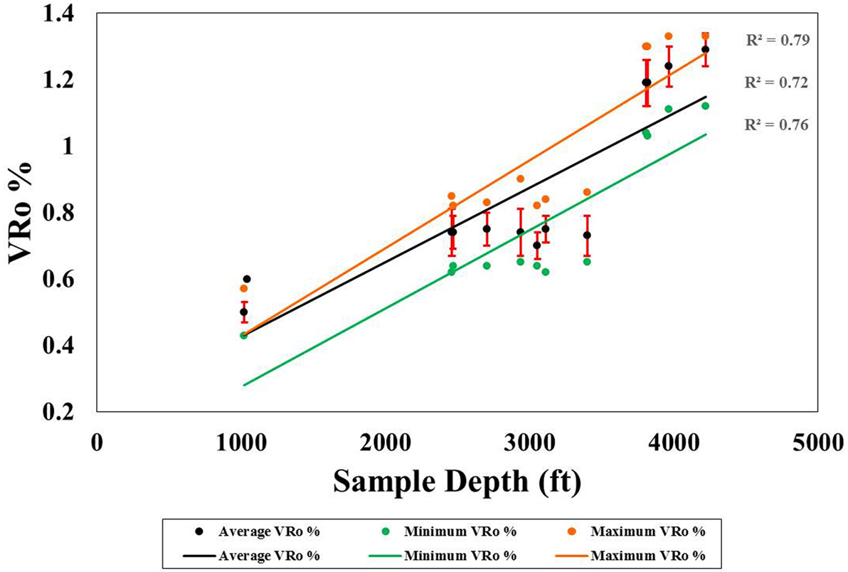
Figure 1. Linear correlations between the minimum (green), average (black), and maximum (orange) vitrinite reflectance values and the measured sample-depth (R² = 0.71). The points representing the Interstate 2460 and Columbia 2471, and the EQT 3809 and 3818 wells overlap due to the proximity of the sample-depths.

In order to develop quantitative correlations using Raman spectral data, a curve/peak-fitting process was evaluated. This method reconstructed the original, experimental Raman spectrum by first automatically finding unambiguous vibrational modes. If the software does not identify all of the peaks, the analyst can manually add subsidiary bands until the summed spectrum of the individual peaks best matches the experimental data. The quality of the fit is visually assessed by evaluating the residual spectrum remaining after the peaks have been fit to the experimental data, and numerically by the χ² metric. The literature illustrating this technique highlights the use of different numbers of peaks to effectively reproduce the original Raman data (Quirico et al., 2005; Bonoldi et al., 2016). In this study, two, five, six, and seven-peak fits were employed to evaluate how the selection of the D, G, and ancillary peaks would affect the linear regressions.

The five baseline-corrected and averaged Raman spectra for each of the 13 shale samples are shown in Figure 2. The visual assessment of the normalized spectra (Figure S3 in Supplementary Material) pointed to two trends: a shift in the D-band maximum to lower frequencies and a narrowing of the G-band full width at half maximum (FWHM). This latter metric can be more readily identified in Figure S3C in Supplementary Material, which provides an enlarged view of the G-band measured for the shallowest and deepest depths of a given well. Figure 3 demonstrates the fitting of (A) two, (B) five, (C) six including a ~1,610 cm⁻¹ peak, (D) six, including a ~1,660 cm⁻¹ peak, and (E) seven peaks to the Raman spectra of an example shale sample. Figure 3 also illustrates how the χ² value decreased with the addition of more peaks, providing a reconstructed spectrum that better resembled the original data. In this plot, the upper red trace represents the reconstructed Raman spectrum, which overlays the original data depicted in Figure 2 and Figure S3 in Supplementary Material. This is exemplified in Figure 3A, where the original blue spectrum can be seen in addition to the red, reconstructed spectrum due to a lower fitting accuracy. The colored peaks below the reconstructed spectrum reveal the individual bands selected for the respective peak-fitting strategy.

FIGURE 2

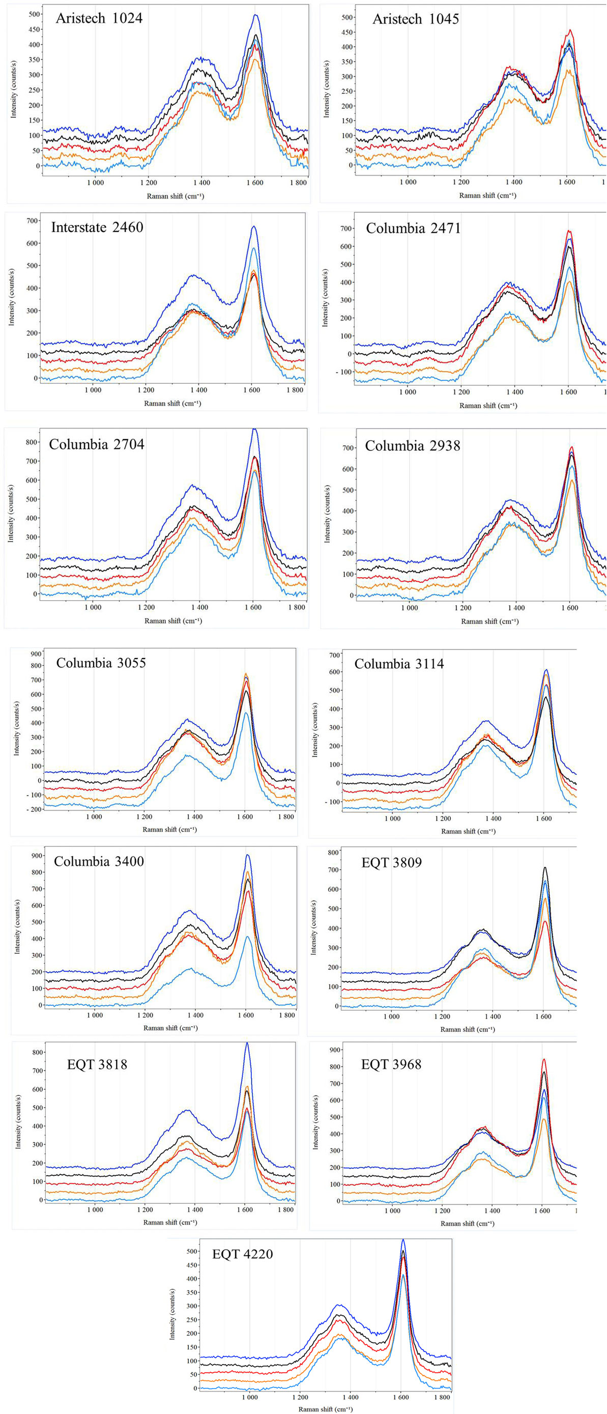
Figure 2. Averaged Raman spectra of 13 shale samples used for peak-fitting. The 100 data points were divided into sets of 20, producing five averaged spectra per sample. Each of the five averaged spectra was individually peak-fit, and the resultant Raman correlations have been provided with corresponding standard deviations.

FIGURE 3

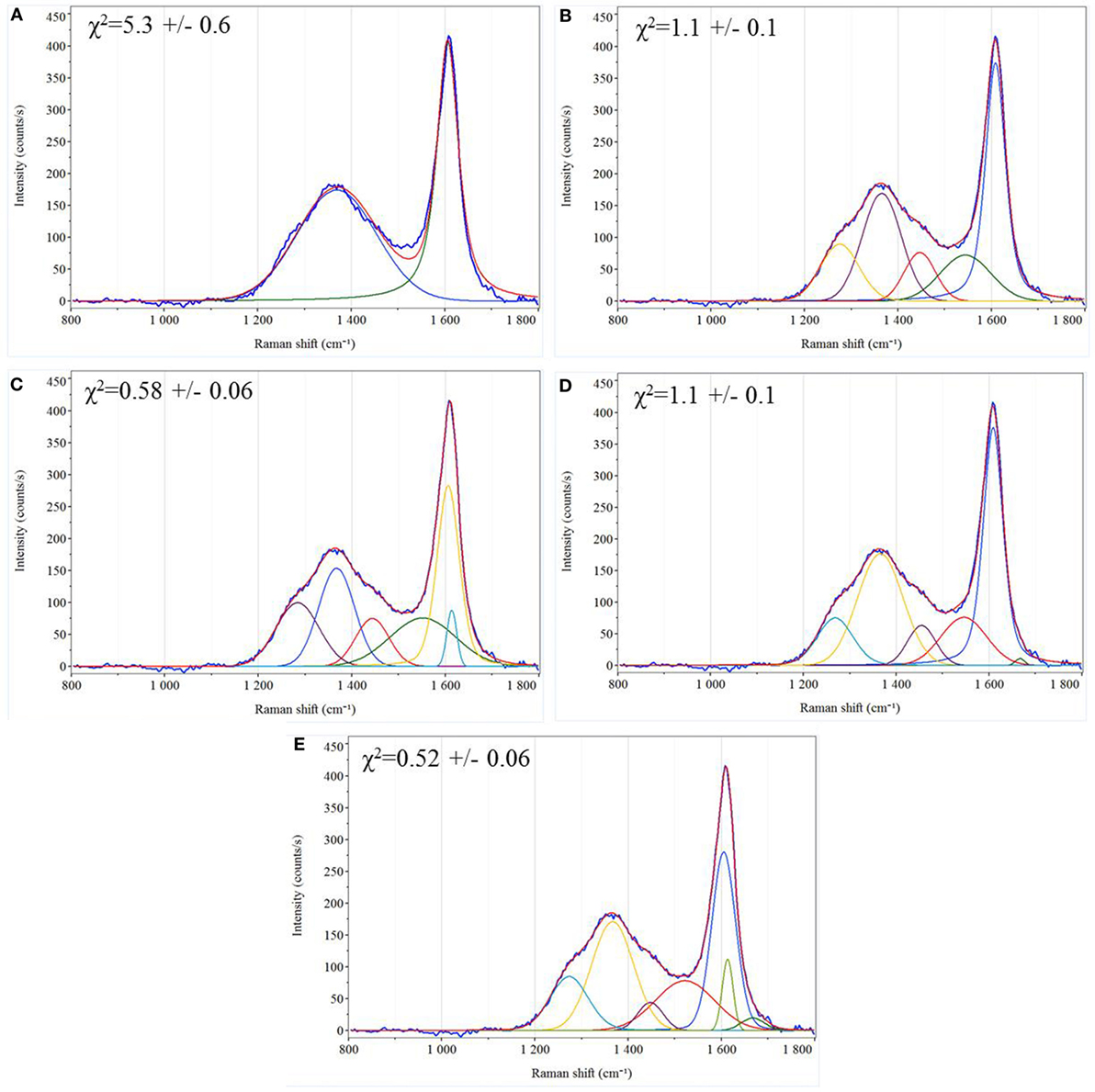
Figure 3. Comparison of peak-fitting iterations using (A) two peaks, (B) five peaks, (C) six peaks, with the sixth located ~1,610 cm⁻¹, (D) six peaks, with the sixth located ~1,660 cm⁻¹, and (E) seven peaks. In each window, the upper, continuous red trace represents the reconstructed Raman spectrum. This trace is overlaid on the original, blue Raman spectrum as shown in Figure 2. The colored traces below the reconstructed spectrum are the individual bands used in the peak-fit.

The metrics determined from each of the peak-fitting strategies employed on the averaged Raman spectra for the 13 shale samples are provided in Table 2. Maximum peak widths of 100 (data not shown) and 200 cm⁻¹ were evaluated to gage how altering this user-defined parameter would affect the resulting correlations. The evaluation of trends exhibiting linearity presented in this manuscript (Figures 4–9; Figures S4–S9 in Supplementary Material) employed a 200 cm⁻¹ maximum peak width, as the use of a 100 cm⁻¹ maximum width resulted in a measured D-band FWHM of 100 cm⁻¹ for nearly every shale sample, thereby unintentionally normalizing the data set to the D-band. Increasing the maximum peak width to 200 cm⁻¹ enabled a more accurate assessment of the actual D-band FWHM. Additionally, any trends developed using both the D- and G-peak metrics when the D-band was inadvertently normalized were expected to and experimentally observed to bias the result to the G-band (data not shown). The χ² values for the peak fits of the shale samples are listed in Table 3. The use of seven peaks clearly demonstrates higher success at reconstructing the original spectra. Relationships between the D- and G-band frequency, the difference in frequency between the D- and G-peaks (band separation), G-FWHM, D/G FWHM ratio, and D/G peak area ratio with thermal maturity were assessed. Tables 4 and 5 provide the coefficients of determination (R²) generated for each attempt at establishing a linear trend between a given metric, different peak-fitting strategies, and VRo or sample-depth, respectively.

TABLE 2

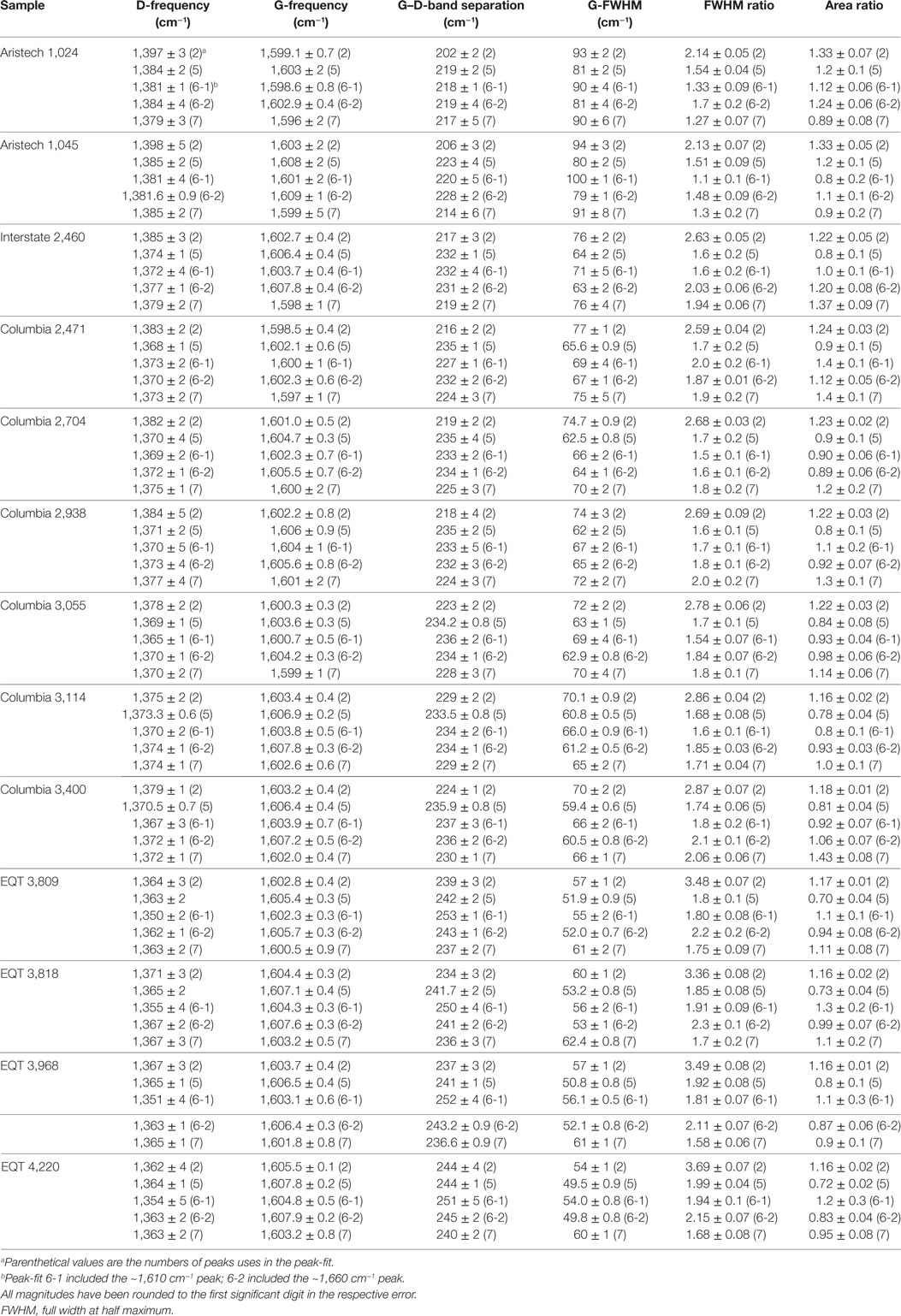
Table 2. Mean Raman spectral peak-fit parameters from five averaged spectra obtained using a 200 cm⁻¹ maximum peak width.

FIGURE 4

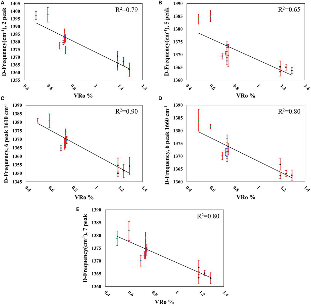
Figure 4. Correlations between D-band frequency and measured VRo% using (A) two peaks (R² = 0.79), (B) five peaks (R² = 0.65), (C) six peaks including the D2-band (R² = 0.90), (D) six peaks including a ~1,660 cm⁻¹ peak (R² = 0.80), and (E) seven peaks (R² = 0.80). Data point legend: green = Aristech wells, blue = Interstate/Columbia wells, black = EQT wells.

FIGURE 5

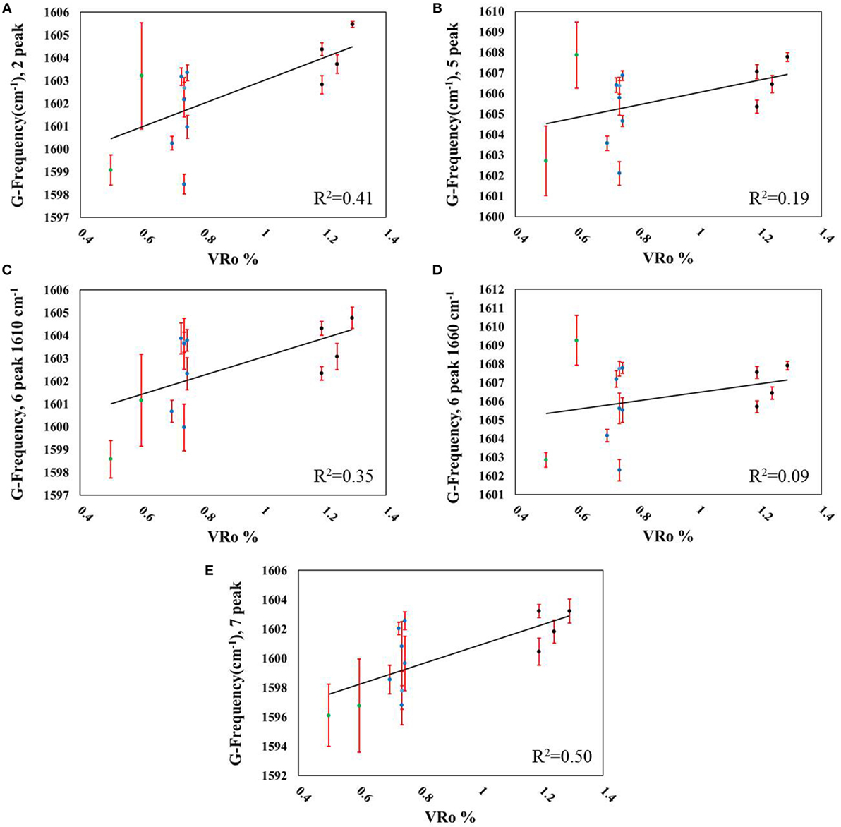
Figure 5. Correlations between G-band frequency and measured VRo% using (A) two peaks (R² = 0.41), (B) five peaks (R² = 0.19), (C) six peaks including the D2-band (R² = 0.35), (D) six peaks including a ~1,660 cm⁻¹ peak (R² = 0.09), and (E) seven peaks (R² = 0.50). Data point legend: green = Aristech wells, blue = Interstate/Columbia wells, black = EQT wells.

FIGURE 6

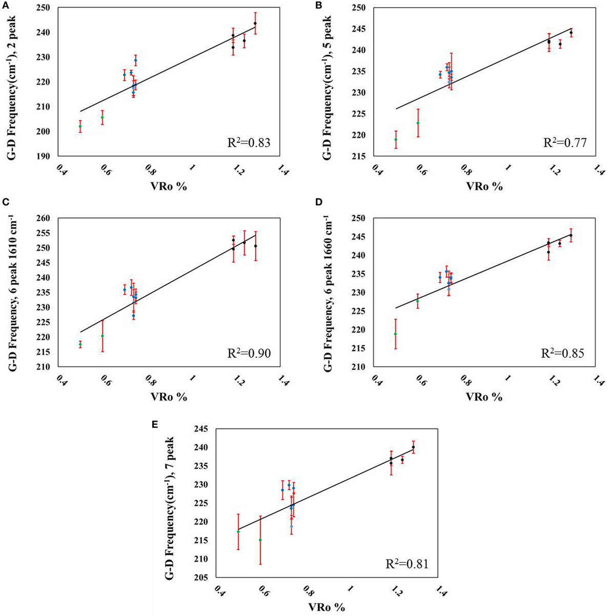
Figure 6. Correlations between G–D-frequency difference and measured VRo% using (A) two peaks (R² = 0.83), (B) five peaks (R² = 0.77), (C) six peaks including the D2-band (R² = 0.90), (D) six peaks including a ~1,660 cm⁻¹ peak (R² = 0.85), and (E) seven peaks (R² = 0.81). Data point legend: green = Aristech wells, blue = Interstate/Columbia wells, black = EQT wells.

FIGURE 7

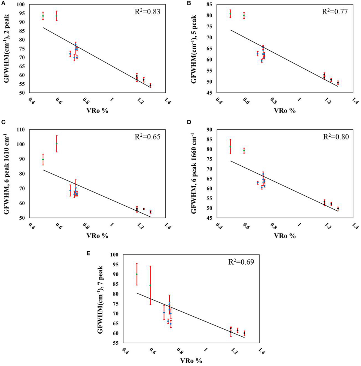
Figure 7. Correlations between G-FWHM and measured VRo% using (A) two peaks (R² = 0.83), (B) five peaks (R² = 0.77), (C) six peaks including the D2-band (R² = 0.65), (D) six peaks including a ~1,660 cm⁻¹ peak (R² = 0.80), and (E) seven peaks (R² = 0.69). Data point legend: green = Aristech wells, blue = Interstate/Columbia wells, black = EQT wells.

FIGURE 8

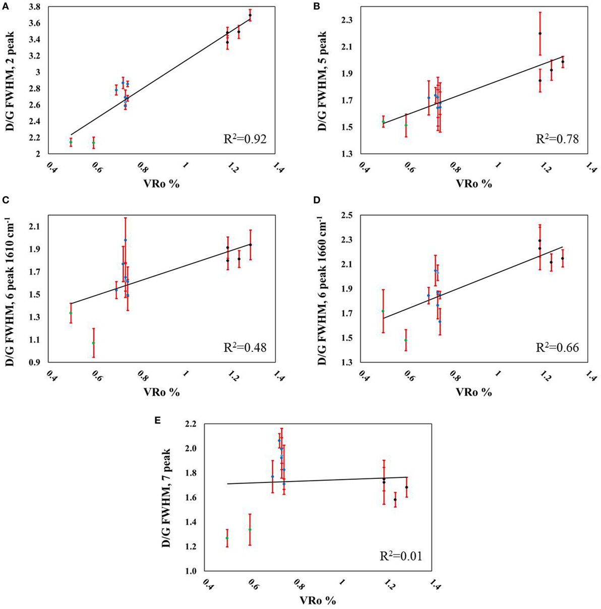
Figure 8. Correlations between D/G full width at half maximum (FWHM) and measured VRo% using (A) two peaks (R² = 0.92), (B) five peaks (R² = 0.78), (C) six peaks including the D2-band (R² = 0.48), (D) six peaks including a ~1,660 cm⁻¹ peak (R² = 0.66), and (E) seven peaks (R² = 0.01). Data point legend: green = Aristech wells, blue = Interstate/Columbia wells, black = EQT wells.

FIGURE 9

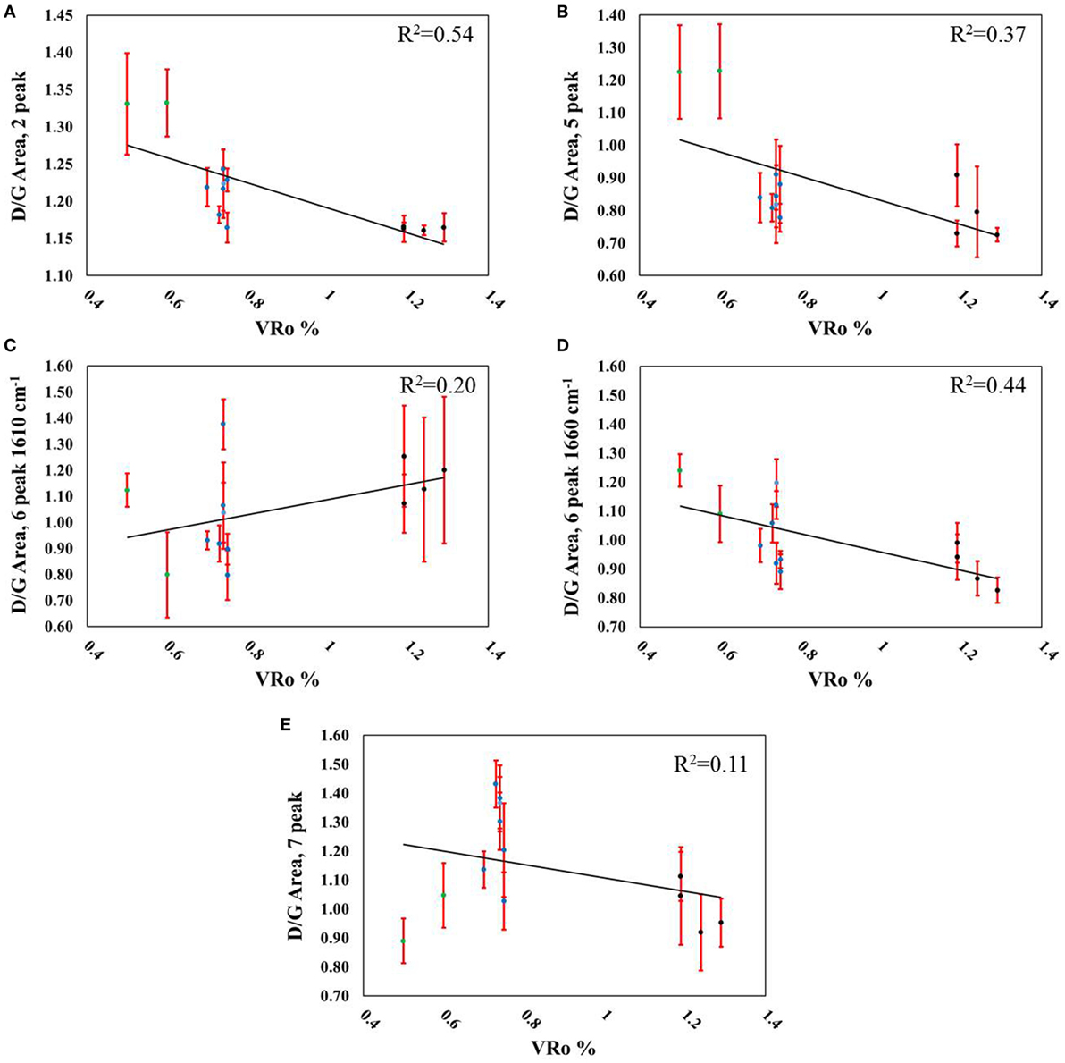
Figure 9. Correlations between D/G peak area and measured VRo% using (A) two peaks (R² = 0.54), (B) five peaks (R² = 0.37), (C) six peaks including the D2-band (R² = 0.20), (D) six peaks including a ~1,660 cm⁻¹ peak (R² = 0.44), and (E) seven peaks (R² = 0.11). Data point legend: green = Aristech wells, blue = Interstate/Columbia wells, black = EQT wells.

TABLE 3

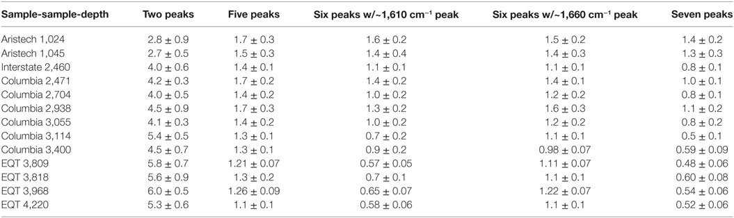
Table 3. Number of peaks selected and resultant χ² values.

TABLE 4

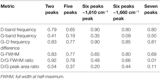
Table 4. Coefficients of determination (R²) generated from correlation of Raman spectral metrics with VRo% using different peak-fitting strategies.

TABLE 5

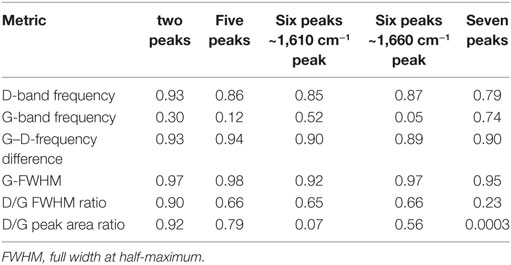
Table 5. Coefficients of determination (R²) generated from correlation of Raman spectral metrics with sample-depth using different peak-fitting strategies.

Initially, two peaks were fit to each spectrum to obtain the maxima of the two main vibrational modes in the Raman data: the D-band, centered between 1,350 and 1,397 cm⁻¹ and the G-band, occurring from 1,596 to 1,609 cm⁻¹, both locations being sample dependent. These G-band peak positions agree with frequencies tabulated in the literature (Table 6) (Wang et al., 1990; Spotl et al., 1998; Matthews et al., 1999; Castiglioni et al., 2001; Beyssac et al., 2002; Quirico et al., 2005; Guedes et al., 2012; Lünsdorf et al., 2014; Li et al., 2015; Lünsdorf, 2016); however, using only one peak to fit the D-band resulted in a shift in the peak maximum location, as shown in Table 2. Limiting the fit to two peaks permitted the bands to be evaluated as a whole, without over-complicating the analysis, and also without needing to add further peaks when the true number of vibrational modes that contribute to the spectral region between ~1,200 and 1,500 cm⁻¹ is unknown. The two-peak fit revealed the same trends visually observed in the spectra shown in Figures S2B,C in Supplementary Material: a shift in the D-band maximum to lower frequencies (Figure 4A), and a narrowing of the G-band FWHM (Figure 7A) with increasing sample-depth. These trends are also provided numerically in Table 2.

TABLE 6

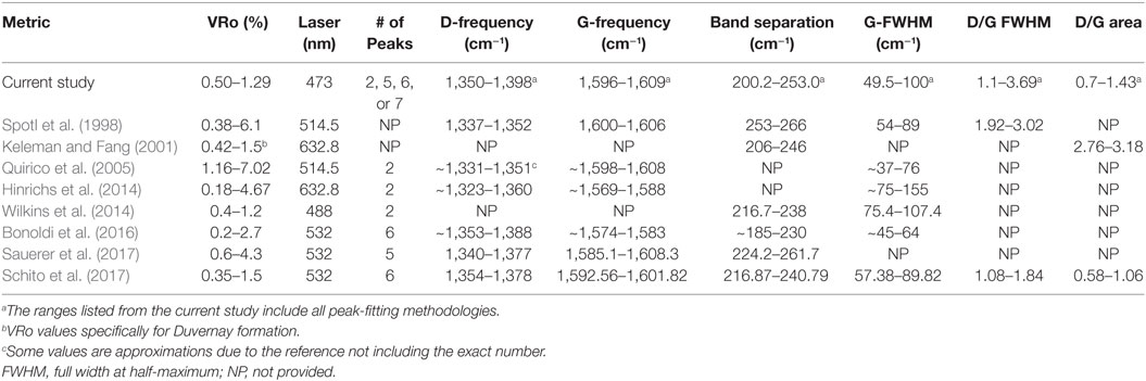
Table 6. Comparison of Raman spectral metrics calculated in the current study with metrics from the literature.

While a two-peak fit elucidated some basic correlations with VRo, it was apparent that additional peaks comprised the spectra, both from the experimental data and the literature (Wang et al., 1990; Matthews et al., 1999; Castiglioni et al., 2001; Beyssac et al., 2002; Jehlička et al., 2003; Quirico et al., 2005; Guedes et al., 2010, 2012; Lünsdorf et al., 2014; Li et al., 2015; Lünsdorf, 2016). Additional peaks were added to the fitting process and were centered between 1,263 and 1,286 cm⁻¹ and 1,430 and 1,466 cm⁻¹, depending on the sample. Peaks near these two spectral locations have been used in several peak-fitting strategies in the literature (Guedes et al., 2012; Lünsdorf et al., 2014; Li et al., 2015; Lünsdorf, 2016). A fifth peak was also added to the valley between the D- and G-modes (centered between 1,495 and 1,578 cm⁻¹). Guedes et al. (2010, 2012) included peaks at 1,465 and 1,540 cm⁻¹ in their spectral characterization. A peak at 1,539 cm⁻¹ was also included by Jehlička et al. (2003) for their fitted spectra. Lünsdorf (2016) also added a peak in this spectral region for their nine peak-fit of coal. The six-peak fit considered either the D2 mode (centered between 1,608 and 1,625 cm⁻¹) or a band in the tail of the G-peak centered between 1,658 and 1,695 cm⁻¹, with the precise location of both peaks dependent on the sample. The latter peak corresponds to C = O bonds, and has been measured in coal using IR and Raman spectroscopy (Guedes et al., 2012; Li et al., 2015). Figures 4A–E demonstrates the linear correlations developed when looking at how the D-band frequency changes with VRo, and different fitting strategies. As can be seen from these figures and Table 4, the addition of more peaks did not necessarily translate to more accurate relationships, as the seven-peak fit provided a lower coefficient of determination (R² = 0.80) than the six-peak fit (using the D2 peak), and the same coefficient of determination as the two- and six-peak (using the ~1,660 cm⁻¹ mode) fits. Despite the lack of change in correlation accuracy with the addition of supplementary peaks, the D-band peak maximum showed a dependence on the depth at which the sample was collected (Table 5). Interestingly, the D-band frequency revealed a stronger correlation with sample-depth (R² = 0.79–0.93, Table 5, Figure S4 in Supplementary Material) compared to VRo (R² = 0.65–0.90, Table 4, Figure 4) across each peak-fitting method.

The G-band frequency did not scale linearly with VRo or sample-depth, with the exception of the seven-peak fit correlated to sample-depth (Figures 5A–E; Figures S5A–E in Supplementary Material; Tables 4 and 5); however, the G- and D-band separation did correlate with the peak-fitting iterations (Figures 6A–E, R² = 0.77–0.90). Again, fitting the original Raman spectra with seven peaks did not lead to the highest coefficient of determination (R² = 0.81). Band separation correlations to sample-depth revealed strong linearity across all of the peak-fitting methods (R² = 0.89–0.94). The G-FWHM metric demonstrated three correlations with VRo greater than R² = 0.77 (Figures 7A,B,D), with the exceptions of the six-peak fit when the D2-band was added to the reconstructed spectrum (R² = 0.65), and the seven-peak fit (R² = 0.69). Similar to the D-band frequency correlations, stronger linear regressions were obtained when the G-FWHM was plotted against sample-depth (Table 5, R² = 0.92–0.98, Figure S7 in Supplementary Material). Intriguingly, the inclusion of the D2-band provided less accurate correlations with VRo for three of the metrics studied when using six peaks to recreate the spectra (Table 5), despite the fact that this peak is consistently demonstrated in the literature. The regression of the metrics generated from the same six peak-fitting strategy with sample-depth resulted in less accurate correlations for nearly every parameter, juxtaposed to the exclusion of this peak. While the addition of the D2-band did lead to similar or better overall peak fits (Table 3), it did not necessarily produce more linear correlations (Tables 4 and 5). One of the most accurate correlations generated, regardless of the thermal maturity parameter employed, using this peak-fitting formula was for the D-frequency (VRo%: R² = 0.90, Table 4, Figure 4C; Sample-depth: R² = 0.85, Table 5; Figure S4C in Supplementary Material). This metric is essentially unrelated to inclusion or exclusion of the D2 peak. The second metric that provided an accurate regression for both VRo and sample-depth when the D2 peak was included in the fit was the band separation (VRo%: R² = 0.90, Table 4, Figure 6C; R² = 0.90, Table 5; Figure S6C in Supplementary Material). This is not surprising given that it is the D-band that shifts with changes in thermal maturity, while the G-band remains relatively stationary (Figure 2, Table 2) (Quirico et al., 2005; Schito et al., 2017). Therefore, most of the differences in band separation stem from the migration of the D-band to lower wavenumbers with increases in thermal maturity.

The ratio of D/G FWHM also revealed a dependence on the peaks used to evaluate the spectral data (Figures 8A–E), as only the use of two (Figure 8A) and five peaks (Figure 8B) led to correlations with VRo greater than 0.78 (R² = 0.92 and 0.78. respectively). These same two-peak fits also provided the strongest correlations with sample-depth (2-peak: R² = 0.90; 5-peak: R² = 0.66) although the six-peak fit that included the ~1,660 cm⁻¹ peak also provided a R² of 0.66 (Table 5). The D/G area ratio (Figures 9A–E) showed the second poorest correlation across the metrics evaluated in this study when correlated to VRo, eclipsed only by the G-band frequency (Table 4). When sample-depth denoted thermal maturity, the D/G area led to the least accurate correlations, with the exceptions of the two-peak fit (R² = 0.92, Table 5), and the five peak-fit (R² = 0.79, Table 5).

Discussion

In this study, Raman spectroscopy was evaluated as a suitable analytical tool for quantifying thermal maturity. Both the measured VRo and sample-depth were employed in the attempt to generate linear correlations between a spectral attribute calculated from peak-fitting the experimental data and thermal maturity. Prior to conducting the peak-fitting analysis, the averaged spectra were baseline-corrected using a linear function. Linear baseline corrections have previously been employed for the analysis of coal and shale Raman spectra (Quirico et al., 2005; Sonibare et al., 2010; Hinrichs et al., 2014; Wilkins et al., 2014; Sauerer et al., 2017). Lünsdorf et al. (2014) discussed the potential bias generated from use of linear and polynomial baseline corrections. The authors state that a “linear baseline is more reproducible” and that a “linear fit is valid if the background can be approximated by a linear baseline.” Sample types were segregated into three “crystallinity levels” based on the morphology of the spectral data. Based off of this spectral classification, a linear baseline fit was found to provide relative SDs of <1% for crystallinity level 1, whereas a curved baseline led to increased variation. The two different baseline correction methods were found to provide similar degrees of variation for crystallinity level 2. The shale samples evaluated in this study possess spectral features representing both crystallinity 1 and 2, since the D2 and D4 shoulders are apparent in the Raman spectra. Given the conclusions drawn by Lünsdorf et al. (2014), the linear baseline correction was selected. The analysis of several different polynomial fits was found to misrepresent the spectral baseline (Figure S2 in Supplementary Material). For example, a fifth order polynomial baseline resolved the trough region between the D and G-bands.

While Raman spectroscopy has shown promise for correlating geological trends, the coefficients of determination in Tables 4 and 5 illustrate how the selection of peak-fitting parameters can significantly affect the results of linear regression. This observation is supported by other studies in the literature (Quirico et al., 2005; Lünsdorf et al., 2014; Lünsdorf and Lünsdorf, 2016). While qualitative trends were observed in the baseline-corrected and normalized spectral data (Figure S3 in Supplementary Material), quantifying these relationships using peak-fitting can be ambiguous, as analysts must determine what acceptable peak widths should be employed, and how many peaks should be used to best signify the original spectra. The addition of more peaks to reduce the peak-fit error (Table 3) did not automatically translate to higher correlative accuracies in the regressed data (Tables 4 and 5). Using seven peaks perplexingly produced only two R² ≥ 0.80 when correlated to VRo, and only two strong correlation (R² ≥ 0.90) when regressed to sample-depth. The two-peak fit led to four correlations with R² ≥ 0.79 with VRo, and five correlations with R² ≥ 0.90, even though this fitting strategy did not portray every vibrational mode. The literature reflects this conundrum, as peak-fitting protocols utilizing 2 to 10 peaks have been published (Quirico et al., 2005; Guedes et al., 2010, 2012; Lahfid et al., 2010; Hinrichs et al., 2014; Lünsdorf et al., 2014; Wilkins et al., 2014; Li et al., 2015; Lünsdorf, 2016; Schito et al., 2017). While more peaks can lead to reduced χ² values, how many peaks accurately represent the sample? The D-band is a complex mixture of vibrational modes. The experimental data herein seems to be comprised of three distinct bands stretching from approximately 1,200–1,500 cm⁻¹; however, there has been no general consensus as to the number of peaks present. Fitting the G-band is less nebulous, as the literature predominantly emphasizes two vibrational modes: the G-band itself, and a shoulder representing the D2 peak. Interestingly, inclusion of this D2 peak led to a less accurate correlation to G-band FWHM, while the inclusion of a peak between 1,662 and 1,689 cm⁻¹ did not hinder the G-band FWHM regression, when regressed to VRo. The six-peak fit that included the D2 mode (Figure 3C) determined that the D2 peak is essentially shrouded by the G-peak, thereby elucidating how the inclusion of the D2 could affect calculated parameters involving G-band widths. The correlations of G-FWHM to sample-depth were all resoundingly robust, as the R² values were greater than 0.9 (Table 5: two-peak = 0.97; five-peak = 0.98; six-peak, ~1,610 cm⁻¹; six-peak, ~1,660 cm⁻¹ = 0.97; seven-peak = 0.95), suggesting that the lack of a linear resolution between VRo values also played a paramount role in the weaker correlations.

In addition to specifying the number of peaks used in the fit, the analyst must also set the maximum peak width the peak-fitting software will employ when reconstructing experimental data. Applying a 100 cm⁻¹ maximum peak width cut off the FWHM of the D-band, as nearly every calculated FWHM for the D-band was 100 cm⁻¹. In some cases, the 100 cm⁻¹ width also cut off the G-band FWHM. In examples where the D-band FWHM was cut, calculated trends indicated that the G-band controlled that metric’s correlation accuracy. While this would be expected when considering G-specific trends, like FWHM, caution must be employed when interpreting metrics like the D/G peak or area ratios.

This research has demonstrated that while trends between Raman data and thermal maturity are observed, subjectivity in data analysis by the analyst may lead to widely different regression trends when reconstructing Raman spectra by peak-fitting. In addition, peak-fitting approaches to developing quantitative trends are hindered by the fact that Raman spectra of shales exhibit changes with thermal maturity, such as the shifting of the D-band, or the narrowing of the G-band. This makes it impossible to employ the same array of fitting parameters across all samples, such as holding the x-axis frequency or FWHM fixed.

Generally, correlations generated by regression to VRo did not provide as accurate of trends as when using sample-depth as a thermal maturity proxy. The D/G FWHM was an exception, as regression of this metric to VRo produced R² values higher than their sample-depth counterparts for four of five fitting strategies. Strong correlations between the D-band frequency and the G-FWHM with sample-depth were measured across most peak-fitting strategies. The data presented herein were compared with several examples of similar studies in the literature (Table 6). It should be noted that these comparisons put the current work in the context of results in the literature, despite differences in samples and spectral acquisition parameters, such as excitation wavelength. The D-band has been shown to be especially sensitive to changes in laser wavelength; therefore, D-frequency comparisons made between studies are for illustrative purposes. Band separation (G-D peak frequency) has been nominated as a useful metric in developing correlations of samples with differing thermal maturities. Band separation values in the current study ranged from 202 ± 2 to 253 ± 1 cm⁻¹. The work by Sauerer et al. (2017) demonstrated the application of band separation to 11 shale samples measured using 532 nm excitation. The band separation ranged from 224.2 to 261.7 cm⁻¹ using a five-peak fit. Band separation values in this study, for a five-peak fit ranged from 219 ± 2 to 244 ± 1 cm⁻¹. While Spotl et al. (1998) did not evaluate band separation, they provided both the D and G peak positions such that the band separation could be calculated. In this example, the values ranged from 253 to 266 cm⁻¹ for the Woodford-Chattanooga kerogen, and 256–263 cm⁻¹ for the Atoka Formation kerogen, both having been analyzed using a 514.5 nm laser. These values, however, did not scale linearly with VRo. Keleman and Fang (2001) also evaluated band separation for a few shale formations evaluated using a 632.8 nm laser. While it is not apparent that the authors used peak-fitting, due to the lack of details provided in the experimental, band separation values ranged from 206 to 246 cm⁻¹, and scaled linearly with VRo. A band separation evaluation of several different types of kerogen by Bonoldi et al. (2016) revealed a range of approximately 185–255 cm⁻¹ that scaled linearly with VRo. The authors used 532 nm excitation, and a six-peak fit. Schito et al. (2017) found band separation values of 216.87–240.79 cm⁻¹ for a series of kerogen samples ranging from 1,290 to 4,950 m deep, using 532 nm excitation, and a six-peak fit.

Individual G-peak positions in this research ranged from 1,596 ± 2 to 1,609 ± 1 cm⁻¹ depending on the peak-fitting protocol. Bonoldi et al. (2016) measured G-peaks from approximately 1,574–1,583 cm⁻¹. The research by Sauerer et al. (2017) revealed G-band frequencies between 1,585.1 and 1,604.3 cm⁻¹. Quirico et al. (2005) measured G-peak positions from approximately 1,598 to 1,608 cm⁻¹. G-positions from 1,600 to 1,606 cm⁻¹ were measured by Spotl et al. (1998), while Schito et al. (2017) detected G-bands from 1,592.56 to 1,601.82 cm⁻¹.

The G-FWHM ranges from the narrowest value of 49.5 ± 0.9 cm⁻¹ for the five-peak fit of the deepest sample to 100 ± 1 cm⁻¹ for the six-peak fit (including the D2-band) for the shallowest sample. Spotl et al. (1998) calculated G-FWHM values ranging from 54 to 89 cm⁻¹, although, again, there was not a linear trend with VRo for these samples. Bonoldi et al. (2016) measured G-FWHM values from 45 to 64 cm⁻¹ for samples with VRo values from approximately 0.5 to 1.9 from their six-peak fit spectra. Six of the samples studied had measured VRo values on par with those contained in the current study. The six-peak fit evaluated herein that most resembles the work by Bonoldi et al. produced G-FWHM values ranging from 55.8 to 104.8 cm⁻¹. While the lower maturity samples herein had much wider peak widths, the samples with the highest VRo values produced very similar results to Bonoldi et al. A G-FWHM range from approximately 37 to 76 cm⁻¹ was measured by Quirico et al. (2005) for coal samples exhibiting VRo values from 1.2 to 7%. Schito et al. (2017) measured G-FWHM of 57.38 to 89.82 cm⁻¹.

The D/G FWHM ratios in the current manuscript range from as low as 1.1 ± 0.1, for the six-peak fit (including the ~1,610 cm⁻¹ peak) of the sample representing the shallowest depth (Table 2) to as high as 3.69 ± 0.07 for the two-peak fit of the sample marking the deepest depth. Spotl et al. (1998) also evaluated the D/G FWHM ratio, and calculated values ranging from 1.92 to 3.02. Schito et al. (2017) measured D/G FWHM from 1.08 to 1.84 with increases in sample-depth using a six-peak-fitting protocol. The authors did not include the known D2-band in their fitting parameters. The shallowest sample by Schito and co-authors measured (1,290 m) matches the deepest sample evaluated in the current study (4,220 ft). The D/G area ratios calculated in this study range from 0.70 ± 0.04 to 1.37 ± 0.09 depending on the peak-fitting method chosen. Schito et al. (2017) also calculated this parameter using the six-peak-fitting protocol, and tabulated values from 0.58 to 1.06.

Using sample-depth as a proxy for thermal maturity has limitations, as any method designed using this metric would be restricted to the specific samples contained in the study and their concomitant geology. However, this metric provided an interesting alternative for tying Raman spectra to thermal maturity for the shale samples evaluated in this research. This study also illustrated that the subjective methods used to develop these correlations can and will influence linear regression. Therefore, employing only one set of experimental peak-fitting parameters and generating correlations from the resultant data may not accurately portray the true relationships between Raman spectra and thermal maturity.

Conclusion

Although some trends were observed when correlating Raman spectral attributes to thermal maturity using both the measured VRo and sample-depths, the obscurities inherent in peak-fitting methods limit the utility and practicality of using this approach to scale Raman data to thermal maturity. Altering one peak-fitting parameter can impede the accuracy of the calibration curve used to quantify properties in unknown samples. The research presented herein has presented circumstances where user interpretation and extrapolation have affected the comparability of different samples, the accuracy of trends generated, and therefore, the utility of the method for becoming an industry benchmark. These results concur with several conclusions drawn in the literature. Since Raman spectroscopy has shown promise in elucidating some basic, qualitative trends with thermal maturity, the generation of Raman techniques that does not require extensive operator interaction and potential manipulation of the data is needed. We are currently developing a more robust, sophisticated, and reproducible Raman spectral and data processing method that provides VRo equivalent values.

Author Contributions

JL developed the method for the spectral analysis, acquired and processed the Raman data, interpreted the results, and drafted the manuscript. LF processed some of the spectral data and aided in the generation of figures for the manuscript. TP, PH, and LS drafted some sections of the manuscript, and provided geological technical details. TP, CE, and PH provided the shale samples with concomitant reference data. SS provided critical editing of the final manuscript and technical support through the project.

Conflict of Interest Statement

The authors declare that the research was conducted in the absence of any commercial or financial relationships that could be construed as a potential conflict of interest.

Acknowledgments

The authors extend our gratitude to the Berea Consortium for providing the shale samples used in this study and to Bryan Bandli, Vince Conrad and Keith Wagner of RJ Lee Group, Inc., Robert Burruss and Clint Scott of the US Geological Survey, and Grant Myers of WellDog, who provided feedback on the manuscript. Any use of trade, firm, or product names is for descriptive purposes only and does not imply endorsement by the U.S. Government.

Supplementary Material

The Supplementary Material for this article can be found online at https://www.frontiersin.org/article/10.3389/fenrg.2017.00024/full#supplementary-material.

References

Araujo, C. V., Borrego, A. G., Cardott, B., das Chagas, R. B. A., Flores, D., Gonçalves, P., et al. (2014). Petrographic maturity parameters of a Devonian shale maturation series, Appalachian Basin, USA. ICCP Thermal Indices Working Group interlaboratory exercise. Int. J. Coal Geol. 130, 89–101. doi: 10.1016/j.coal.2014.05.002

CrossRef Full Text | Google Scholar

ASTM. (2015). D 7708 Standard Test Method for Microscopical Determination of the Reflectance of Vitrinite Dispersed in Sedimentary Rocks, Petroleum Products, Lubricants, and Fossil Fuels; Gaseous Fuels; Coal and Coke. West Conshohocken, PA: ASTM International.

Google Scholar

Berea Consortium Release. (2017). Berea Consortium Release. Available at: http://www.uky.edu/KGS/news/berea-consortium-release-2017.php

Google Scholar

Beyssac, O., Goffé, B., Chopin, C., and Rouzaud, J. N. (2002). Raman spectra of carbonaceous material in metasediments: a new geothermometer. J. Metamorph. Geol. 20, 859–871. doi:10.1046/j.1525-1314.2002.00408.x

CrossRef Full Text | Google Scholar

Bonoldi, L., Di Paolo, L., and Flego, C. (2016). Vibrational spectroscopy assessment of kerogen maturity in organic-rich source rocks. Vibr. Spectrosc. 87, 14–19. doi:10.1016/j.vibspec.2016.08.014

CrossRef Full Text | Google Scholar

Carr, A. D., and Williamson, J. E. (1990). The relationship between aromaticity, vitrinite reflectance and maceral composition of coals: implications for the use of vitrinite reflectance as a maturation parameter. Org. Geochem. 16, 313–323. doi:10.1016/0146-6380(90)90051-Z

CrossRef Full Text | Google Scholar

Castiglioni, C., Mapelli, C., Negri, F., and Zerbi, G. (2001). Origin of the D line in the Raman spectrum of graphite: a study based on Raman frequencies and intensities of polycyclic aromatic hydrocarbon molecules. J. Chem. Phys. 114, 963–974. doi:10.1063/1.1329670

CrossRef Full Text | Google Scholar

Chen, Y., Zou, C., Mastalerz, M., Hu, S., Gasaway, C., and Tao, X. (2015). Applications of micro-Fourier transform infrared spectroscopy (FTIR) in the geological sciences – a review. Int. J. Mol. Sci. 16, 30223–30250. doi:10.3390/ijms161226227

CrossRef Full Text | Google Scholar

Cole, G. A., Drozd, R. J., Sedivy, R. A., and Halpern, H. I. (1987). Organic geochemistry and oil-source correlations, paleozoic of Ohio. AAPG Bulletin 71(7), 788–809.

Google Scholar

Dow, W. G. (1977). Kerogen studies and geological interpretations. J. Geochem. Explor. 7, 79–99. doi:10.1016/0375-6742(77)90078-4

CrossRef Full Text | Google Scholar

East, J. A., Swezey, C. S., Repetski, J. E., and Hayba, D. O. (2012). Thermal Maturity Map of Devonian Shale in the Illinois, Michigan, and Appalachian Basins of North America: U.S. Geological Survey Scientific Investigations. Reston, VA: USGS.

Google Scholar

Ferrari, A. C., and Robertson, J. (2000). Interpretation of Raman spectra of disordered and amorphous carbon. Phys. Rev. B 61, 14095–14107. doi:10.1103/PhysRevB.61.14095

CrossRef Full Text | Google Scholar

Guedes, A., Valentim, B., Prieto, A. C., and Noronha, F. (2012). Raman spectroscopy of coal macerals and fluidized bed char morphotypes. Fuel 97, 443–449. doi:10.1016/j.fuel.2012.02.054

CrossRef Full Text | Google Scholar

Guedes, A., Valentim, B., Prieto, A. C., Rodrigues, S., and Noronha, F. (2010). Micro-Raman spectroscopy of collotelinite, fusinite and macrinite. Int. J. Coal Geol. 83, 415–422. doi:10.1016/j.coal.2010.06.002

CrossRef Full Text | Google Scholar

Hackley, P. C., Araujo, C. V., Borrego, A. G., Bouzinos, A., Cardott, B. J., Cook, A. C., et al. (2015). Standardization of reflectance measurements in dispersed organic matter: results of an exercise to improve interlaboratory agreement. Marine Petrol. Geol. 59, 22–34. doi:10.1016/j.marpetgeo.2014.07.015

CrossRef Full Text | Google Scholar

Hackley, P. C., Ryder, R. T., Trippi, M. H., and Alimi, H. (2013). Thermal maturity of northern Appalachian Basin Devonian shales: insights from sterane and terpane biomarkers. Fuel 106, 455–462. doi:10.1016/j.fuel.2012.12.032

CrossRef Full Text | Google Scholar

Hinrichs, R., Brown, M. T., Vasconcellos, M. A. Z., Abrashev, M. V., and Kalkreuth, W. (2014). Simple procedure for an estimation of the coal rank using micro-Raman spectroscopy. Int. J. Coal Geol. 136, 52–58. doi:10.1016/j.coal.2014.10.013

CrossRef Full Text | Google Scholar

Hunt, J. M. (1979). “The source rock,” in Petroleum Geochemistry and Geology (San Francisco: William H. Freeman and Company), 261–350.

Google Scholar

Jacob, H. (1989). Classification, structure, genesis and practical importance of natural solid oil bitumen (“migrabitumen”). Int. J. Coal Geol. 11, 65–79. doi:10.1016/0166-5162(89)90113-4

CrossRef Full Text | Google Scholar

Jehlička, J., Urban, O., and Pokorný, J. (2003). Raman spectroscopy of carbon and solid bitumens in sedimentary and metamorphic rocks. Spectrochim. Acta Mol. Biomol. Spectrosc. 59, 2341–2352. doi:10.1016/S1386-1425(03)00077-5

PubMed Abstract | CrossRef Full Text | Google Scholar

Keleman, S. R., and Fang, H. L. (2001). Maturity trends in Raman spectra from kerogen and coal. Energy Fuels 15, 653–658. doi:10.1021/ef0002039

CrossRef Full Text | Google Scholar

Lahfid, A., Beyssac, O., Deville, E., Negro, F., Chopin, C., and Goffé, B. (2010). Evolution of the Raman spectrum of carbonaceous material in low-grade metasediments of the Glarus Alps (Switzerland). Terra Nova 22, 354–360. doi:10.1111/j.1365-3121.2010.00956.x

CrossRef Full Text | Google Scholar

Li, K., Khanna, R., Zhang, J., Barati, M., Liu, Z., Xu, T., et al. (2015). Comprehensive investigation of various structural features of bituminous coals using advanced analytical techniques. Energy Fuels 29, 7178–7189. doi:10.1021/acs.energyfuels.5b02064

CrossRef Full Text | Google Scholar

Li, X., Hayashi, J.-I., and Li, C. Z. (2006). FT-Raman spectroscopic study of the evolution of char structure during the pyrolysis of a Victorian brown coal. Fuel 85, 1700–1707. doi:10.1016/j.fuel.2006.03.008

CrossRef Full Text | Google Scholar

Lo, H. B. (1993). Correction criteria for the suppression of vitrinite reflectance in hydrogen-rich kerogens: preliminary guidelines. Org. Geochem. 20, 653–657. doi:10.1016/0146-6380(93)90051-C

CrossRef Full Text | Google Scholar

Lo, H. B., and Cardott, B. J. (1995). Detection of natural weathering of Upper McAlester coal and Woodford Shale, Oklahoma, U.S.A. Org. Geochem. 22, 73–83. doi:10.1016/0146-6380(95)90009-8

CrossRef Full Text | Google Scholar

Lünsdorf, N. K. (2016). Raman spectroscopy of dispersed vitrinite – methodical aspects and correlation with reflectance. Int. J. Coal Geol. 153, 75–86. doi:10.1016/j.coal.2015.11.010

CrossRef Full Text | Google Scholar

Lünsdorf, N. K., Dunkl, I., Schmidt, B. C., Rantitsch, G., and von Eynatten, H. (2014). Towards a higher comparability of geothermometric data obtained by Raman spectroscopy of carbonaceous material. Part I: evaluation of biasing factors. Geostand. Geoanal. Res. 38, 73–94. doi:10.1111/j.1751-908X.2013.12011.x

CrossRef Full Text | Google Scholar

Lünsdorf, N. K., and Lünsdorf, J. O. (2016). Evaluating Raman spectra of carbonaceous matter by automated, iterative curve-fitting. Int. J. Coal Geol. 160–161, 51–62. doi:10.1016/j.coal.2016.04.008

CrossRef Full Text | Google Scholar

Matthews, M. J., Pimenta, M. A., Dresselhaus, G., Dresselhaus, M. S., and Endo, M. (1999). Origin of dispersive effects of the Raman D band in carbon materials. Phys. Rev. B 59, R6585–R6588. doi:10.1103/PhysRevB.59.R6585

CrossRef Full Text | Google Scholar

McCreery, R. L. (2000). “Magnitude of Raman scattering,” in Raman Spectroscopy for Chemical Analysis, ed. J. D. Winefordner (New York: John Wiley & Sons, Inc.), 15–33.

Google Scholar

Mukhopadhyay, P. K. (1994). “Vitrinite reflectance as maturity parameter,” in Vitrinite Reflectance as a Maturity Parameter, eds P. K. Mukhopadhyay, W. G. Dow (Washington, DC: American Chemical Society), 1–24.

Google Scholar

Quirico, E., Raynal, P.-I., and Bourot-Denise, M. (2003). Metamorphic grade of organic matter in six unequilibrated ordinary chondrites. Meteorit. Planet. Sci. 38, 795–811. doi:10.1111/j.1945-5100.2003.tb00043.x

CrossRef Full Text | Google Scholar

Quirico, E., Rouzaud, J.-N., Bonal, L., and Montagnac, G. (2005). Maturation grade of coals as revealed by Raman spectroscopy: progress and problems. Spectrochim. Acta Mol. Biomol. Spectrosc. 61, 2368–2377. doi:10.1016/j.saa.2005.02.015

PubMed Abstract | CrossRef Full Text | Google Scholar

Rahl, J. M., Anderson, K. M., Brandon, M. T., and Fassoulas, C. (2005). Raman spectroscopic carbonaceous material thermometry of low-grade metamorphic rocks: calibration and application to tectonic exhumation in Crete, Greece. Earth Planet. Sci. Lett. 240, 339–354. doi:10.1016/j.epsl.2005.09.055

CrossRef Full Text | Google Scholar

Repetski, J. E., Ryder, R. T., Weary, D. J., Harris, A. G., and Trippi, M. H. (2008). “Thermal maturity patterns (CAI and %R_o) in Upper Ordovician and Devonian rocks of the Appalachian basin: a major revision of USGS Map I–917–E using new subsurface collections,” in U.S. Geological Survey Scientific Investigations Map 3006. Available at: https://pubs.usgs.gov/sim/3006/

Google Scholar

Sauerer, B., Craddock, P. R., AlJohani, M. D., Alsamadony, K. L., and Abdallah, W. (2017). Fast and accurate shale maturity determination by Raman spectroscopy measurement with minimal sample preparation. Int. J. Coal Geol. 173, 150–157. doi:10.1016/j.coal.2017.02.008

CrossRef Full Text | Google Scholar

Schito, A., Romano, C., Corrado, S., Grigo, D., and Poe, B. (2017). Diagenetic thermal evolution of organic matter by Raman spectroscopy. Org. Geochem. 106, 57–67. doi:10.1016/j.orggeochem.2016.12.006

CrossRef Full Text | Google Scholar

Schmidt, J. S., Hinrichs, R., and Araujo, C. V. (2017). Maturity estimation of phytoclasts in strew mounts by micro-Raman spectroscopy. Int. J. Coal Geol. 173, 1–8. doi:10.1016/j.coal.2017.02.003

CrossRef Full Text | Google Scholar

Smith, E., and Dent, G. (2005). “Introduction, basic theory and principles,” in Modern Raman Spectroscopy: A Practical Approach (Chichester: Wiley), 1–22.

Google Scholar

Sonibare, O. O., Haeger, T., and Foley, S. F. (2010). Structural characterization of Nigerian coals by X-ray diffraction, Raman and FTIR spectroscopy. Energy 35, 5347–5353. doi:10.1016/j.energy.2010.07.025

CrossRef Full Text | Google Scholar

Spotl, C., Houseknecht, D. W., and Jaques, R. C. (1998). Kerogen maturation and incipient graphitization of hydrocarbon source rocks in the Arkoma Basin, Oklahoma and Arkansas: a combined petrographic and Raman spectrometric study. Org. Geochem. 28, 535–542. doi:10.1016/S0146-6380(98)00021-7

CrossRef Full Text | Google Scholar

Suárez-Ruiz, I., Flores, D., Mendonça Filho, J. G., and Hackley, P. C. (2012). Review and update of the applications of organic petrology: part 1, geological applications. Int. J. Coal Geol. 99, 54–112. doi:10.1016/j.coal.2012.02.004

CrossRef Full Text | Google Scholar

Taylor, G. H., Teichmüller, M., Davis, A., Diessel, C. F. K., Littke, R., and Robert, P. (1998). Organic Petrology. Berlin and Stuttgart: Gebruder Borntraeger.

Google Scholar

Wang, Y., Alsmeyer, D. C., and McCreery, R. L. (1990). Raman spectroscopy of carbon materials: structural basis of observed spectra. Chem. Mater. 2, 557–563. doi:10.1021/cm00011a018

CrossRef Full Text | Google Scholar

Wilkins, R. W. T., Boudou, R., Sherwood, N., and Xiao, X. (2014). Thermal maturity evaluation from inertinites by Raman spectroscopy: the ‘RaMM’ technique. Int. J. Coal Geol. 128–129, 143–152. doi:10.1016/j.coal.2014.03.006

CrossRef Full Text | Google Scholar

Zhou, Q., Xiao, X., Pan, L., and Tian, H. (2014). The relationship between micro-Raman spectral parameters and reflectance of solid bitumen. Int. J. Coal Geol. 121, 19–25. doi:10.1016/j.coal.2013.10.013

CrossRef Full Text | Google Scholar