Data assimilation: making sense of Earth Observation

Introduction

Important societal challenges of the Twenty-first Century include climate change, air quality, and environmental degradation (IPCC, 2013). These challenges have a strong impact on society, incurring significant social and economic costs (Lahoz et al., 2012, and references therein). To address these challenges we need information on the Earth System, the main elements being the atmosphere, ocean, land surface, and cryosphere. Variables of interest include temperature, winds, and atmospheric constituents (atmosphere); sea surface temperature and ocean salinity (ocean); land surface temperature and soil moisture, and snow cover (land surface); and glacier elevation and velocity (cryosphere). The spatial scales range from 100 s of meters, or less (e.g., urban centers) to ~10,000 km (e.g., global scales); the temporal scales range from 1 h or less (e.g., atmospheric pollutants) to centuries and longer (e.g., ocean currents and glaciers). A set of these variables have been classified as GCOS (Global Climate Observing System) essential climate variables (ECVs¹) to support the work of the UNFCCC (United Nations Framework Convention on Climate Change) and the IPCC (Intergovernmental Panel on Climate Change).

We have two broad sources of information of the Earth System: measurements, i.e., “observations”; and understanding of the spatio-temporal evolution, typically embodied in “models,” e.g., representing equations describing relationships between variables and/or parameters. From the point of view of the spatio-temporal evolution of the Earth System, observations and models are not distinct; it is the mechanism of obtaining this information that is distinct: observations have a roughly direct link with the Earth System via the measurement process; models have a roughly indirect link with the Earth System, being an embodiment of information received from measurements, experience, and theory. The observational and model information has uncertainty, and a key task is to understand and quantitatively estimate this uncertainty.

Information on the Earth System from observations and models allows society to take action to address the challenges it faces. For example, it allows society to prepare for the future behavior of the Earth System (“prediction”); to test our understanding of the Earth System, and adjust this understanding (“hypothesis testing”); and to record and evaluate changes in the Earth System, and assess compliance with environmental legislation (“monitoring”).

The methods used to observe the Earth System using instrumentation include (Lahoz, 2010; Thépaut and Andersson, 2010): in situ observations from ground-based stations, buoys and aircraft; and satellite observations from low Earth orbit satellites (LEOs) and geostationary satellites (GEOs)—satellites in highly elliptic orbits (HEOs) are also being considered to observe the Arctic (Masutani et al., 2013). Collectively, these observational platforms are termed the Global Observing System (GOS). The in situ and satellite observational platforms are complementary (USGEO, 2010): in situ platforms have relatively high spatio-temporal resolution, but do not have global coverage; satellite platforms have substantial coverage over the globe, for LEOs this coverage being quasi-global, but have relatively poor spatio-temporal resolution. In situ data and ground-based remote sensing data, are often used to evaluate and calibrate (using these data as unbiased, anchor data) satellite data for the various elements of the Earth System.

The satellite observations considered in this review come from operational and research satellites. Operational satellites are mainly used for weather forecasting, and research satellites are mainly used for research of the Earth System. However, the distinction between operational and research satellites is becoming blurred, as more research satellites are used operationally for weather forecasting. Currently, satellite observations used operationally by the weather centers are dominated by nadir-viewing satellites; limb-viewing satellites are also used (Thépaut and Andersson, 2010).

Many operational satellite instruments measure infrared or microwave radiation from the atmosphere and the Earth's surface. These data provide information on the temperature and humidity of the atmosphere, the temperature and emissivity of the surface, as well as clouds and precipitation which all affect the measured radiances. Research satellite instruments measure radiation that provides information on the various elements of the Earth System, including the atmosphere (dynamical variables, atmospheric composition); the ocean (sea surface temperature and salinity); the land surface (soil moisture, snow); and the cryosphere (marine ice thickness).

While the observations mentioned above are usually taken by specialized entities such as the space agencies (Thépaut and Andersson, 2010), a novel and recent development in platforms for observing the Earth System is provided by activities from citizens involved in science, i.e., Citizen Science (Science Communications Unit, 2013). Citizen Science activities have been described as people accumulating knowledge in order to learn about and respond to environmental threats (Irwin, 1995), and as public participation in scientific research (Rosner, 2013). Associated with Citizen Science is the concept of crowdsourcing, defined to be “the act of taking a job traditionally performed by a designated agent (usually an employee) and outsourcing to an undefined, generally large group of people in the form of an open call” (Howe, 2010).

Examples of Citizen Science activities in the environmental sciences date back to at least the Nineteenth Century. Recent examples include observations by amateurs of birds (Sullivan et al., 2009) and butterflies (van Swaay et al., 2008) to assess the health of the environment. The advent of technologies such as the internet and smartphones, and the growth in their usage², has significantly increased the potential benefits from Citizen Science activities. These technologies provide an opportunity to extend the range of observational platforms available to society and, in particular, at spatio-temporal scales (10 s of meters; 1 h or less) that are highly relevant to the needs of the citizen. These activities may include mass participation schemes in which citizens use smartphones to submit observational information on their immediate environment, e.g., on air quality and meteorological conditions. The potential value of Citizen Science is high, with applications in science, education, social aspects, and policy aspects, but this potential, particularly for citizens and policymakers, remains largely untapped. Notable challenges associated with Citizen Science activities include quality of data from low-cost sensors, and concerns about data security and data privacy.

Although observations are essential to estimate the state of the Earth System, they are characterized by two key limitations. The first one is that they contain errors—these can be systematic (also called bias), random, and of representativeness (see Cohn, 1997; Lahoz, 2010; Ménard, 2010). The sum of these errors is sometimes known as the accuracy. Random errors have the property that they are reduced by averaging. Systematic errors, by contrast, are not reduced by averaging; if known, they can be subtracted from an observation. The representativeness error is associated with differences in the resolution of observational information and the resolution in the way this information is interpreted. The second limitation is that they have spatio-temporal gaps (Lahoz et al., 2010a)—see Figure 1. It is necessary to fill in the gaps in the information provided by observations: (i) to make this information more complete, and hence more useful; and (ii), to provide information at a regular scale to allow easier quantification of physical processes, e.g., calculation of fluxes between the land and the atmosphere. Information at an irregular scale can be used to quantify physical processes, but this procedure is more tractable when done at a regular scale.

FIGURE 1

Figure 1. Plot representing typical data gaps in satellite observations of tropospheric composition, illustrated using night-time total column carbon monoxide (CO) (units of molecules cm⁻²) retrieved over Asia using data from the Measurements Of Pollution In The Troposphere (MOPITT) instrument on 17 January 2014. The figure shows both gaps between the swaths of the satellite platform as well as missing data points due to clouds and/or other measurement issues within each swath. Red colors indicate relatively high CO total column; blue colors indicate relatively low CO total column.

To fill in the gaps in the observations a model is needed (Lahoz et al., 2010a). This model can be simple, e.g., linear interpolation or geostatistical approaches based on the spatial and temporal autocorrelation of the observations, or take account of the system's behavior. For example, the model could be a chemistry-transport model (CTM), incorporating a suite of chemical equations and heterogeneous chemistry (Errera et al., 2008); could be a general circulation model (GCM), incorporating the discretized Navier–Stokes equations (Salby, 1996); or could be a land surface model (LSM) incorporating the transports of energy between the land surface and the atmosphere (Lahoz and De Lannoy, 2014). The model thus extends the observations, fills in the observational gaps and allows one to organize, summarize, and propagate the information from observations. The model, like the observations, also exhibits gaps in space and time.

It is desirable to find methods that allow the interpolation, i.e., filling in of the observational information gaps using a model, to be done in an “intelligent” way. By intelligent, we mean an “objective” way which makes use of concepts for combining information that can be quantified. For example, by finding the state that minimizes a “penalty function” calculated from observational information and prior information (e.g., from a model forecast). We can think of the model used for the forecast as an intelligent interpolator of the observational information: intelligent because it embodies our understanding of the system; intelligent because the combination of the observational and the model information is done in an objective way. A methodology that allows this intelligent interpolation is data assimilation (Kalnay, 2003; Lahoz et al., 2010b).

In this review paper we discuss the data assimilation methodology in section Data Assimilation Methodology. In section Applications of Data Assimilation we discuss its applications and successes, providing examples that span a broad range of features of the Earth System. We then discuss the outlook and challenges for data assimilation including the novel application of using Citizen Science as a source of environmental information (section Outlook). Section Conclusion provides conclusions.

Data Assimilation Methodology

Background

Mathematics provides rules for combining information objectively, based on principles which aim to maximize (or minimize) a quantity (e.g., a “penalty function”), or on established statistical concepts which relate prior information (understanding, which comes from prior combination of observations and models) with posterior information (which comes from making an observation). It provides a foundation to address questions such as: “What combination of the observation and model information is optimal?” Mathematics also helps in defining in an objective way the meaning of “optimum,” in estimating the errors of the “optimum” estimate, and in measuring “optimality.” This is known as “data assimilation,” and has strong links to several mathematical disciplines, including control theory and Bayesian estimation (Nichols, 2010).

Data assimilation adds value to the observations by filling in the observational gaps, and adds value to the model by constraining it with observations (Lahoz et al., 2010a)—see Figure 2. This allows self-consistent and realistic representation of the Earth System on a regular grid (in Figure 2 the stratospheric ozone distribution). In this way, data assimilation allows one to “make sense” of Earth Observation. In particular, data assimilation provides methods for combining in an objective way observations and models with different spatio-temporal characteristics and errors: local footprint vs. quasi-global footprint; local coverage vs. global coverage; differences in sampling frequency; and errors arising from matching different spatio-temporal scales. An example of how data assimilation combines heterogeneous observational and model information is provided by the weather forecasting agencies (Kalnay, 2003). The result of data assimilation, where observational and model information and their errors, are combined, is termed the “analysis.” When the data assimilation approach is performed for past data covering a long time period (e.g., one or more decades of years) using a consistent system, the result is termed a “reanalysis” (Bengtsson and Shukla, 1988; Trenberth and Olson, 1988).

FIGURE 2

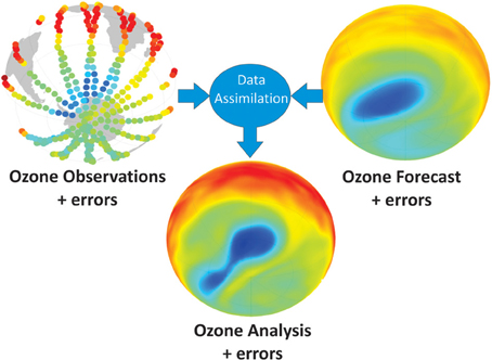
Figure 2. Schematic of how data assimilation adds value to observational and model information. The data shown are various representations of the ozone distribution at 10 hPa (~30 km) on 23 September 2002, each of which has errors. Upper left panel: plot representing ozone data from a limb-viewing satellite. Upper right panel: plot representing a 6-day ozone forecast based on output from a data assimilation system. Bottom panel: plot representing an ozone analysis based on output from a data assimilation system. Blue colors represent relatively low ozone values; red/orange colors represent relatively high ozone values. The analysis is produced by combination of the observational and model information and their errors. Note how the analysis fills in the observational data gaps and captures the Antarctic ozone split, verified using independent data not used in the assimilation. By contrast, the ozone hole split is not captured in the 6-day ozone forecast. Based on material in Lahoz et al. (2010a).

In data assimilation, the observations, models, and analyses have errors, which will never be known precisely, and which have to be estimated. This means the data assimilation problem has to be stated in probabilistic terms (see, e.g., Cohn, 1997). Figure 2 shows this graphically, with information from observations, models and their errors, input into the data assimilation algorithm, and producing an analysis, which also has errors.

The objective combination of information from a model and from observations can be formulated mathematically using Bayesian estimation ideas (Rodgers, 2000). The starting point is Bayes's theorem, which relates the posterior probability of an event A, given that event B is known to have occurred, P(A|B), to the prior probability of A, P(A), multiplied by the probability of B occurring given that A is known to have occurred, P(B|A):

$\begin{array}{cc}P\left(A|B\right)=\alpha P(A)P\left(B|A\right),& (1)\end{array}$

where α is a normalizing constant that ensures that Equation (1) defines a probability measure.

The formulation in Equation (1) can be applied to a general state of the Earth System, e.g., the atmosphere, where A is the event x = x^t, i.e., x is the true state, x^t, and B is the event y = y⁰, i.e., observations, y, are given by y⁰ (we use notation standard in the data assimilation literature; see Lorenc, 1986; Nichols, 2010). Because the truth is not known, it is common to consider estimates of the state x given its deviations from a background (a priori) state, x^b, (x – x^b), and its deviations from the observations, or measurements, y⁰, (y⁰ – H(x)), where H is a non-linear observation operator (to be specified later) that maps information from the space of x to the space of y⁰. The state x^b is commonly estimated from a short model forecast; this embodies the model information. With this formulation, Equation (1) defines a multi-dimensional probability distribution function (PDF), P^a = P(A|B), related to PDFs representing errors in the prior (model) information (P(x– x^b) = P(A)), and errors in the observational information (P(y⁰ − H(x)|x − x^b) = P(B|A), including errors in the mapping effected by H). The state x (the analysis, see sections Variational Methods and Sequential Methods), which is what we are interested in, can be estimated using notions of minimum variance (estimation of the mean) or maximum a posteriori (estimation of the mode) applied to the PDF, P^a (Nichols, 2010).

Although Bayesian estimation defines a systematic and rigorous approach to data assimilation (Rodgers, 2000; Evensen, 2007), its full-scale implementation in many areas, including weather forecasting, is impossible, chiefly due to the size of the problem. The typical dimension of current weather forecasting models is ~ 10⁷ elements, while the number of observations available over 24 h is ~ 10⁶–10⁷ (Lahoz et al., 2007). As a result, error covariance matrices for the model and observational information have ~ 10¹⁴ elements. However, the Bayesian approach is still useful in that it provides general guidelines for developing a data assimilation system and evaluating its results. Nevertheless, in many practical applications it is necessary to make simplifying assumptions to the data assimilation methodology. Two main lines have been followed: (i) statistical linear estimation (discussed in sections Variational Methods and Sequential Methods), and (ii) ensemble assimilation (discussed in section Ensemble Methods). The representation of errors in data assimilation is discussed in section Representation of Errors.

Statistical linear estimation achieves Bayesian estimation when the system is linear and the errors are Gaussian. In particular, statistical linear estimation provides a way of estimating the Best Linear Unbiased Estimate (BLUE) (Nichols, 2010). The data assimilation problem of finding the analysis, x, can be related to finding the minimum value of a penalty function involving the prior information, x^b, and the observational information, y⁰, introduced above. In general, this is a non-linear problem, and explicit solutions cannot be found. However, a “best” linear estimate of the solution can be derived explicitly, by linearizing the problem about the non-linear trajectory of the background, x^b. If additional assumptions are made about the errors in the observational and model information, the solution of the data assimilation problem can be interpreted in statistical terms and the uncertainty in the analysis can be derived. In particular, if we assume that the errors in the observational and model information are randomly distributed and unbiased, and that these errors are uncorrelated, the BLUE equals a least-square estimate for the analysis, x, with minimum variance. When these errors are assumed to be Gaussian, the solution to the data assimilation problem is also equal to the maximum a posteriori Bayesian estimate.

There exist two broad classes of numerical algorithms for data assimilation: variational and sequential (Bouttier and Courtier, 1999). In the context of statistical linear estimation, these algorithms take respectively the form of the 4-D variational method (4D-Var)—see section Variational Methods, or the Kalman filter (KF)—see section Sequential Methods. These are two different algorithms for determining the BLUE, and they are equivalent only under the condition of linearity.

Variational Methods

To illustrate variational algorithms in data assimilation, we first describe the 3-D variational method (3D-Var), which is a particular case of the 4D-Var method in which the temporal dimension of the observations is excluded. In 3D-Var, a minimization algorithm is used to find a model state, x (termed the analysis, x^a), that minimizes the misfit between x and the background state x^b, and also between x and the observations, y, taking into account that x and y can be in different spaces, e.g., reflecting different spatio-temporal characteristics (this is achieved by the observation operator, introduced below). The background state is commonly derived from a short-range forecast (of order a few hours), and is a manifestation of a priori knowledge of the system under consideration. In 3D-Var, we seek the minimum with respect to x of the penalty function, J [error terms and operators in Equation (2) are described below]:

$\begin{array}{cc}J=\frac{1}{2}{\left[x\text{-}{x}^b\right]}^T{B}^{-1}\left[x-x^b\right]+\frac{1}{2}{\left[y-H\left(x\right)\right]}^T{R}^{-1}\left[y-H\left(x\right)\right].& (2)\end{array}$

The first term on the right-hand-side of Equation (2), J_b, quantifies the misfit to the background and the second term, J_o, is the misfit to the observations (see Figure 3). Extra terms incorporating dynamical constraints are also added in some implementations of 3D-Var. The non-linear observation operator, H, maps the model state x to the measurement space, where y resides. If the observation operator is linear (written H), the penalty function, J, is quadratic and is guaranteed to have a unique minimum. The solution of Equation (2) is discussed in Bouttier and Courtier (1999).

FIGURE 3

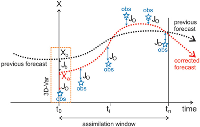
Figure 3. Schematic diagram illustrating 4D-Var. Over the period of the assimilation window indicated 4D-Var is performed to assimilate the most recent observations (marked as blue stars), using a segment of the previous forecast as the background (black line—the background state x^b is the initial condition). This updates the initial model trajectory for the subsequent forecast (red line), using the analysis x^a as the initial condition. The box to the left identifies the special case of 3D-Var. Similar material can be found in http://www.ecmwf.int.

Examples of the role played by H include: (i) a mapping (e.g., a linear interpolation) between model values of an atmospheric parameter (e.g., ozone, water vapor) and observations of these parameters as 3-D height-resolved retrievals or as 2-D retrieved columns; and (ii) a radiative transfer model (often simplified to allow fast and efficient application of the methodology) mapping model values of an atmospheric parameter to observed radiances. Assimilation of retrievals, associated with (i) above, is closer to the model variables and so tends to have a simpler operator H but may have to assume prior knowledge which may be inconsistent with the model. In particular, the prior constraint used in the retrieval to obtain the observations y may be inconsistent with the prior information used in the data assimilation method. Assimilation of radiances, associated with (ii) above, has simpler error characteristics and generally does not have implicit prior knowledge assumed. Radiance assimilation has been shown to improve the overall skill of weather forecasts (Saunders et al., 1999; McNally et al., 2006). Migliorini (2011) provides a rigorous and comprehensive discussion of the conditions for the equivalence between radiance and retrieval assimilation. In particular, it is shown that two requirements need to be satisfied for equivalence: (i) the radiance observation operator, H, needs to be approximately linear in a region of the state space centered at the retrieval and with a radius of the order of the retrieval error; and (ii) both the prior constraint used to determine the retrieval and the prior used for radiance assimilation are chosen so as to not lose the information content of the measurements.

Following Ide et al. (1997), the term B in Equation (2) is the background error covariance matrix representing the errors in the background state; an extension of the Ide terminology to cover ensemble methods (section Ensemble Methods) has been proposed³. The off-diagonal elements of B determine how information is spread spatially from observation locations. If the background errors of one variable are uncorrelated with any other variable, then the analysis is termed “univariate,” but if the errors in different variables are correlated, the analysis is termed “multivariate.” If B is multivariate, it can provide statistical links between dynamical variables, for example, geostrophic coupling, or links between dynamical and chemical variables or different chemical species. Bannister (2008a,b) discusses how to construct B.

The term R in Equation (2) is the observation error covariance matrix representing the errors in the observations. Typically, R is assumed to be diagonal; although this is not always justified, e.g., different elements of a retrieved profile are likely to have correlated errors. R includes the errors of the measurements themselves, E, and errors of representativeness, F; R = E + F. F includes errors in the observation operator, H, and errors arising because the assimilation model does not fully resolve the scales measured by the observations (Cohn, 1997). It is generally assumed that B and R are uncorrelated, i.e., the errors in the model (background) and observational information are uncorrelated.

4D-Var is a development of 3D-Var in which the temporal dimension is included (Bouttier and Courtier, 1999). The minimization is carried out over a time window that is typically 6 or 12 h, although longer time windows have been used, e.g., for chemical data assimilation (Lahoz et al., 2007; Errera et al., 2008). In 4D-Var, observations are used at their correct time. Experiments at the European Centre for Medium-Range Weather Forecasts (ECMWF) suggest this is the main reason for the improved performance in 4D-Var, as compared to 3D-Var (Fisher and Andersson, 2001). A variant of the variational method, 3D-FGAT (First Guess at the Appropriate Time), in which the second term in the right-hand-side of Equation (2) is calculated by comparing observations with the background at the relevant observation times, is described in Fisher and Andersson (2001).

To make variational methods more efficient, an “incremental” approach is generally used in which the non-linear assimilation problem is replaced by a sequence of approximately linear least-squares problems (Courtier et al., 1994). More details of the incremental approach can be found in Nichols (2010). Other techniques to increase the efficiency of 4D-Var, control variable transforms and model reduction, are discussed in Nichols (2010).

4D-Var has two new features compared to 3D-Var. First, it includes a non-linear model operator, M, that carries out the evolution forward in time. The first derivative of M, M, is the tangent linear model (if M is linear, represented by M, its derivative is M). The transpose of the tangent linear model operator, M^T, integrates the adjoint variables backward in time (see Talagrand, 2010a, for a description of adjoint variables). The tangent linear model is only defined under the condition that the function, J, defined by Equation (2) be differentiable—this is the tangent linear hypothesis (see Bouttier and Courtier, 1999, for further details). Second, J can include an extra term in which the model errors associated with the model's temporal evolution are accounted for. For example, in the formulation of Zupanski (1997) an analogous term involving Q⁻¹, z^T Q⁻¹ z, is included in J, where Q is the model error covariance and z represents model errors, e.g., the difference between model states at times t_k and t_k+1. Constructing Q is a research topic. In strong-constraint 4D-Var, the term in the penalty function involving Q⁻¹ is excluded—this assumes a perfect model; in weak-constraint 4D-Var this term is included (Sasaki, 1970a,b,c).

The properties of the adjoint method allow it to play two important roles in 4D-Var: coupling different elements of the algorithm, and computing gradients associated with the minimization of the penalty function (Talagrand, 2010a). The first property allows unobserved regions to be constrained by observed regions; the second property allows efficient computation of the gradient of the penalty function, J.

To illustrate 4D-Var, Figure 3 shows a schematic diagram of the model trajectory and the observations used to update it. The special case of 3D-Var is illustrated by the rectangle to the left of the diagram. The terms J_b and J_o in Equation (2) are also identified.

The applicability of 4D-Var has been demonstrated for weather forecasting (Simmons and Hollingsworth, 2002). The main advantage of 4D-Var is that it considers observations over a time window that is generally much longer than the model time step, i.e., it is a smoothing algorithm. This allows more observations to constrain the system and, considering satellite coverage, increases the geographical area influenced by the data. For non-linear systems, this feature of 4D-Var, together with the non-diagonal nature of the adjoint operator, transfers information from observed regions to unobserved regions. This transfer of observational information reduces the role of the background information, and is manifested in a reduction of the weight of the background error covariance matrix, B, in the final 4D-Var analysis compared to the KF analysis. For linear systems, the general equivalence between 4D-Var and the KF implies that the same weight is given to all data in both systems.

In contrast to the above advantages of 4D-Var, three weaknesses must be mentioned. First, its numerical cost is very high compared to approximate versions of the KF or ensemble methods. Second, its formalism cannot determine the analysis error directly; rather, it has to be computed from the inverse of the Hessian matrix, a procedure which is prohibitive in both computation time and memory. Finally, its formalism requires the calculation of the adjoint model, which is time-consuming and may be difficult for a system such as the land surface which exhibits non-linearities and on–off processes (e.g., presence or lack of snow).

Sequential Methods

To illustrate sequential algorithms in data assimilation, we first describe the KF method (Kalman, 1960). In the KF, a recursive sequential algorithm is applied to evolve a forecast (typically short-range), x^f, and an analysis, x^a, as well as their respective error covariance matrices, P^f and P^a. The KF equations are (subscripts denote time-step):

$\begin{array}{cc}{x}_n^f=M_{n-1}{x}_{n-1}^a;& (3a)\end{array}$

$\begin{array}{cc}{P}_n^f=M_{n-1}{P}_{n-1}^a{M}_{n-1}^T+Q_{n-1};& (3b)\end{array}$

$\begin{array}{cc}{x}_n^a=x_n^f\text{+}{K}_n\left[y_n-H_n{x}_n^f\right];& (3c)\end{array}$

$\begin{array}{cc}{K}_n=P_n^f{H}_n^T{\left[R_n\text{+}{H}_n{P}_n^f{H}_n^T\right]}^{-1};& (3d)\end{array}$

$\begin{array}{cc}{P}_n^a=\left[I\text{-}{K}_n{H}_n\right]P_n^f.& (3e)\end{array}$

Equation (3a) represents the forecast of the model fields from time-step n - 1 to n, while Equation (3b) calculates the forecast error covariance from the analysis error covariance P^a and the model error covariance Q. Equations (3c) and (3e) are the analysis steps, using the Kalman gain defined in Equation (3d). Q and P^a are assumed to be uncorrelated, i.e., the errors in the model and the analysis are uncorrelated. For optimality, all errors must be uncorrelated in time. The forecast term in the KF (Equations 3b, 3c) plays the same role as the background term in 3D-Var (Equation 2). The terms H and M have been introduced in the discussion about 4D-Var. The model error term Q in Equation (3b) plays the same role as the Q term introduced in the formulation of Zupanski (1997) in 4D-Var.

The word “filter” as applied to the KF characterizes an assimilation technique that uses only observations from the past to perform the analysis (Bouttier and Courtier, 1999). An algorithm that uses observations from both the past and the future is called a “smoother.” 4D-Var can be regarded as a smoother. The KF smoother version is called the Kalman smoother (Jazwinski, 1970). The equivalence between the Kalman smoother and weak-constraint 4D-Var has been discussed by Fisher et al. (2005).

A variant of the KF is the Physical-space Statistical Analysis Scheme, PSAS (Cohn et al., 1998). This consists of solving the second term in the right-hand-side of Equation (3c) in observation space instead of in model space. The PSAS approach is efficient for systems where the number of observations is much smaller than the dimension of the model state space.

The KF can be generalized to non-linear H and M operators, although in this case neither the optimality of the analysis nor the equivalence with 4D-Var holds. The resulting equations are known as the Extended Kalman filter, EKF (Bouttier and Courtier, 1999).

The cost of the KF or EKF is much larger than that of 4D-Var, even with small models. This is a consequence of the explicit calculation of P^f, and necessary storage costs. Consequently, development of KF techniques in applications such as chemical data assimilation has tended to focus on approximate methods, based on the hypothesis of model linearity. The time window over which observations can be considered should be chosen carefully to ensure that the linearity hypothesis is satisfied. Khattatov et al. (1999) provide evidence that for a stratospheric photochemical box model, the linear approximation essential to applicability of the EKF is valid up to ~10 days.

Parametrization of the error covariance matrices reduces the cost of the KF; this approach, referred to as the reduced, suboptimal, or modified KF, has been applied to chemical data assimilation. P^f can be constructed by computing the diagonal elements and parametrizing the off-diagonal elements using adjustable parameters for the correlation lengths (Khattatov et al., 2000; Ménard and Chang, 2000; Ménard et al., 2000). Q can be specified by assuming that diagonal elements are proportional to the modeled field itself; they are used to update the diagonal elements of P^f. This approach results in substantial savings, and allows the off-diagonal elements to be computed using a simple relation.

Eskes et al. (2003) developed a KF approach to produce near real time ozone analyses and 5-day forecasts. To comply with limited computer resources and the constraints of an operational service, they introduced several approximations in the KF method. For example, they used observation minus forecast statistics (see Lahoz and Errera, 2010) to estimate the horizontal error correlations, the observation errors, and the forecast errors.

The EKF has been used for the land surface. Examples are provided by Boulet et al. (2002), Reichle et al. (2002), Matgen et al. (2010), and Rüdiger et al. (2010). de Rosnay et al. (2014) show that using the EKF instead of optimal interpolation improves significantly the soil moisture analysis at ECMWF (as determined by comparison against ground-truth data).

A recent development which aims to overcome the shortcoming that the KF and the EKF become impractical for high dimensional systems is the Variational Kalman Filter, VKF (Auvinen et al., 2009). The VKF, and a Variational Kalman smoother (VKS) version, have been tested with numerical examples, and shown to give comparable results to those obtained using the standard KF and EKF (Auvinen et al., 2009). An extension of the VKF to ensemble filtering is described in Solonen et al. (2012). Using numerical examples, it is shown that this ensemble method performs better than the standard Ensemble Kalman filter (EnKF) (section Ensemble Methods), especially for small size ensembles.

Ensemble Methods

Ensemble assimilation is a form of Monte-Carlo approximation which attempts to estimate the PDFs using a finite number of elements. In the EnKF (Evensen, 2003), a Monte-Carlo ensemble of short-range forecasts is used to estimate P^f, the forecast error in the KF (Equation 3b). In the EnKF, the size of the analyzed ensembles typically lies between a few tens to a few hundreds of model states. The estimation becomes more accurate as the ensemble size increases. The EnKF is more general than the EKF to the extent that it does not require validity of the tangent linear hypothesis. The EnKF is attractive as, for example, it requires no derivation of a tangent linear operator or adjoint equations and no integrations backward in time, as for 4D-Var (Evensen, 2003). Several authors (e.g., Lorenc, 2003; Kalnay et al., 2007) have compared 4D-Var and the EnKF, with an emphasis on their suitability for weather forecasting.

Advances in the EnKF include the square-root filter (Anderson, 2001; Whitaker and Hamill, 2002), the Ensemble Transform Kalman filter, ETKF (Bishop et al., 2001) and local Ensemble Kalman filtering (Ott et al., 2004; Hunt et al., 2007). More recent developments include a deterministic formulation of the EnKF (Sakov and Oke, 2008), and an iterative EnKF for non-linear systems (Sakov et al., 2012b). The Ensemble Kalman smoother, EnKS (Evensen and van Leeuwen, 2000; Evensen, 2003), is an extension of the EnKF where information at assimilation times is propagated backward in time, i.e., estimates at times t ≤ t_n, contain information from all data up to and including t_n. Several issues need to be considered in developing the EnKF (Kalnay, 2010): (1) ensemble size; (2) ensemble collapse; (3) correlation model for P^f, including localization; and (4) specification of model errors. To illustrate the concept of the EnKF, Figure 4 shows a diagram of the model trajectories and observations used to update it.

FIGURE 4

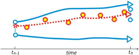
Figure 4. Schematic showing the main elements of the EnKF, as implemented during the assimilation window (t_n−1, t_n). The blue unfilled circles to the left represent the range of the ensemble of analyses at time t_n−1; the full blue lines represent the range of ensemble forecasts using the ensemble of analyses at t_n−1 as the initial states; the dashed red line represents a linear combination of the forecasts (using the red star as the initial state) used to provide the final state—the analysis, at time t_n. The red stars filled in yellow color represent the observations used during the assimilation window. The blue unfilled circles to the right represent the range of the ensemble of analyses at time t_n used for the next assimilation window. The spread of the ensemble members represents the forecast error. Based on material in Kalnay (2010).

Representation of Errors

Representation of errors, including systematic, random, and of representativeness is a key area of data assimilation (Lahoz et al., 2010b). Desroziers et al. (2005) provides a method to evaluate observational, model, and analyses errors. Other methods to evaluate these errors are discussed in Talagrand (2010b). In general, in data assimilation, random errors for the observations and the background or model, are assumed to be Gaussian. The most fundamental justification for assuming Gaussian errors is the relative simplicity and ease of implementation of statistical linear estimation under these conditions. Because Gaussian PDFs are fully determined by their mean and covariance (which might include correlations between the matrix elements), the solution of the data assimilation problem becomes computationally practical. Another argument for the choice of Gaussian errors is that of all possible PDFs with given mean and covariance, the Gaussian distribution has maximum entropy (Rodgers, 2000).

Typically, there are biases between different observations types, and between the observations and the model. Ménard (2010) discusses bias estimation in data assimilation. Biases are spatially and temporally varying and it is a major challenge to estimate and correct them. Despite this, and mainly for pragmatic reasons, in data assimilation it is often assumed that observations are unbiased. For weather forecasting many assimilation schemes now incorporate a bias correction, and various techniques have been developed to correct observations to remove biases (Dee, 2005). These schemes are adaptive, and are designed to be consistent, flexible, and automated. In an adaptive bias correction scheme, the state vector, x (which is what we seek), is augmented to include bias parameters, which can be estimated and adjusted during the assimilation; the bias parameters must be observable. A scheme such as variational bias correction (Dee, 2004) works well when there is sufficient redundancy in the data, or there are no significant model biases. Bias correction methods are also applied to other areas of data assimilation such as the land surface (De Lannoy et al., 2007a,b).

Besides assuming that observations have random errors that are Gaussian, and are unbiased, assimilation methods also assume that observations have no serious errors due to malfunction of instruments, incorrect readings, and software errors. Several methods have been developed to detect (and reject, if necessary) data having such errors (Andersson and Thépaut, 2010). The innovation vector, y – H(x^b), is a measure of the departure of the observations from the background state. It is used to assess whether any serious errors contaminate observational information. The innovation thus provides the basis for several quality control procedures: the first-guess check; buddy checks; optimal interpolation checks; Bayesian methods; and variational quality control. Because the misfit between observations and the background could be large if the observations are in error, or if the background is in error, or both, care must be taken to not reject observations because the background is poor, e.g., in the neighborhood of storms. Thus, good representation of background error characteristics is very important for the success of quality control procedures (Dee et al., 2001). Both bias correction and quality control of observations are crucial for the successful implementation of data assimilation systems.

The major drawback of the algorithms discussed above (variational methods; sequential methods; ensemble methods such as the EnKF) is the underlying assumption that the model states have a Gaussian distribution. The EKF is capable of handling some departure from Gaussian distributions of model errors and non-linearity of the model operator. However, if the model becomes too non-linear or the errors become highly skewed or non-Gaussian, the trajectories computed by the EKF will become inaccurate.

A development in data assimilation using ensemble methods that addresses non-linear and non-Gaussian aspects is the particle filter, PF (van Leeuwen, 2009). An advantage of the PF is that it does not require a specific form for the state distribution, so there is no need to assume a Gaussian distribution. The PF has been shown to perform well in small dimensional systems (Doucet et al., 2001, and references therein). The difficulty in using it for geophysical applications is the large dimensionality of these systems. In high dimensional systems the PF suffers from filter degeneracy. This results in the distribution of weights becoming skewed, so that a re-sampling algorithm needs to be applied. All statistical information on the posterior distribution is lost and there is no longer any advantage in using the PF compared to other data assimilation methods. This prevents the PF being considered as a realistic alternative for data assimilation (Snyder et al., 2008).

Recent research on the PF has focused on trying to ensure that, whilst the ensemble of model runs still represents the prior knowledge of the system, they also represent samples from the high probability region of the posterior distribution (Chorin and Tu, 2009; Bocquet et al., 2010; Chorin et al., 2010; Morzfeld et al., 2012). Another recent development is the equivalent-weights PF (van Leeuwen, 2010, 2011; Ades and van Leeuwen, 2013, 2014). This method avoids degeneracy and thus is able to represent a posterior distribution with many modes—multi-modality is problematic for 3D- and 4D-Var, since there is no guarantee that a global, rather than a local, mode will be found via the gradient methods used to find the minimum of the penalty function.

Because PF methods typically make no assumptions of linearity in the model equations or that model and observational errors are Gaussian, they are well-suited to deal with systems such as the land surface where model evolution is highly non-linear, and model and observational errors can be non-Gaussian. As a result, the PF has been applied in hydrology to estimate model parameters and state variables (Moradkhani et al., 2005a; Weerts and El Serafy, 2006; Plaza et al., 2012; Vrugt et al., 2012).

Complementarity between the EnKF and the PF makes a hybrid approach highly attractive for systems that can exhibit non-linear and non-Gaussian features, for example the land surface. For example, the EnKF could be used as an efficient sampling tool to create an ensemble of particles with optimal characteristics with respect to observations. The PF methodology could then be applied on that ensemble afterwards to resolve non-linearity and non-Gaussianity in the system (see Kotecha and Djurić, 2003).

Applications of Data Assimilation

Introduction

Data assimilation has been applied with success in many areas, a notable example being weather forecasting (also known as numerical weather prediction, NWP). Over the last 25 years, the skill of weather forecasts has increased significantly—for example, the skill of today's 5-day forecast is comparable to the skill of the 3-day forecast 25 years ago (Buizza, 2013). Details of the role data assimilation has played in this improvement can be found in Simmons and Hollingsworth (2002). A historical overview of NWP, including developments in data assimilation, is provided by Kalnay (2003).

The atmosphere, like any dynamical system with instabilities, has a finite limit of predictability even if the model is perfect and the initial conditions are known almost perfectly (Lorenz, 1963a,b; Kalnay, 2003). Lorenz estimated this limit to be about 2 weeks. This feature of the atmosphere is associated with the notion of chaos, and reflects that unstable systems have a finite limit of predictability; conversely, stable systems are infinitely predictable as they are either stationary or periodic. Kalnay (2003) reviews the fundamental concepts of chaotic systems.

The realization that the atmosphere is chaotic has profoundly affected the development of weather forecasting by recognizing that this requires replacement of single “deterministic” forecasts by “ensembles” of forecasts with perturbations in the initial conditions and model characteristics that realistically reflect uncertainties in our knowledge of the atmospheric state. This led to the introduction of operational ensemble forecasting at both NCEP (National Centers for Environmental Prediction) and ECMWF in 1992. The need to obtain the best possible initial conditions to be perturbed for an ensemble forecast provides a strong motivation for the use of data assimilation for weather forecasting.

In recent years, the usefulness of weather forecasts has been extended through systematic exploitation of the chaotic nature of the atmosphere, an example being the development and application of various techniques (adjoint model; Lyapunov vectors; singular vectors; tangent linear model) to operational ensemble forecasting (Kalnay, 2003). Efforts on weather forecast models are now being applied to climate models through notions that predictability can be considered as a seamless weather-climate prediction problem, and that there can be predictive power on all temporal scales (Palmer et al., 2008; Hoskins, 2013).

Details of the application of data assimilation methods, particularly to weather forecasting, were provided at the Sixth WMO (World Meteorological Organization) Data Assimilation Symposium held in October 2013⁴. At these symposium several advanced methods were presented, including weak-constraint 4D-Var (see section Variational Methods), 4D-Ensemble-Var (e.g., Fairbairn et al., 2014), and variants of the EnKF (see section Ensemble Methods). There was no consensus on the best approach, but there was more emphasis on the development of ensemble data assimilation methods and hybrid methods than on the traditional 4D-Var methodology, which has dominated over the past decade. Methods such as iterated EnKFs and PF approaches (see section Representation of Errors) are being examined as possible methods that could be applied to future systems.

Data assimilation is not just applied to weather forecasting; it is also applied to other areas of the Earth System, with insights from the work of the weather centers being helpful. Examples include the design of the GOS using observing system simulation experiments, OSSEs; chemical data assimilation; air quality forecasting; land surface data assimilation; ocean data assimilation; and the production of reanalyses for studying the Earth Climate System. Concerning challenges in data assimilation (see section Challenges in Data Assimilation), applications in one area can benefit from issues already known in other areas; in this way, developments at the weather centers provide strong guidance to developments in other areas where data assimilation is applied.

We now illustrate in more detail applications of the data assimilation methodology using several examples. These include: (i) OSSEs for monitoring air quality (section Observing System Simulation Experiments for Monitoring Air Quality); (ii) ozone data assimilation (section Ozone Data Assimilation); and (iii) land surface data assimilation (section Land Surface Data Assimilation). In section Other Applications of Data Assimilation we discuss other applications of the data assimilation method: general atmospheric chemistry assimilation, ocean assimilation and wave assimilation, and reanalyses.

Applications discussed in sections Observing System Simulation Experiments for Monitoring Air Quality–Other Applications of Data Assimilation are selected to cover a wide range of features representing elements of the Earth System or the observation types providing information on the Earth System. The variety in features includes: (i) spatial scales, from relatively large scales in the stratosphere to relatively small scales in the troposphere, and, similarly, from relatively high heterogeneity in the land surface to relatively low heterogeneity in the atmosphere; (ii) temporal scales, from relatively short scales in the atmosphere to relatively long scales in the ocean; (iii) observation types, from current to planned satellite missions; and (iv) analysis types, from estimates of the best current state (analyses) to estimates of the best state over a past period (reanalyses).

Observing System Simulation Experiments for Monitoring Air Quality

Air quality is defined by the atmospheric composition of gases (e.g., ozone) and particulates (e.g., particulate matter, PM) near the Earth's surface (McNair et al., 1996; Brasseur et al., 2003). Monitoring air quality requires an observing system comprised of satellite and in situ observational platforms (Lahoz et al., 2012). Setting up this observational infrastructure requires the capability to design it in an objective way. Particular questions of interest concerning air quality are the relative contribution of satellite and in situ platforms to the observational information on air quality, and the optimum design of the GOS for monitoring air quality in a cost-effective way.

A methodology for addressing these questions is that of OSSEs—see Figure 5. The OSSE is similar to the observing system experiment, OSE. An OSE considers the impact of existing observations, whereas an OSSE considers the impact of future observations. The OSE results are evaluated against the experiment incorporating all data; the OSSE results are evaluated against the Nature Run, i.e., the Truth (this is illustrated in Figure 6, below). Owing to the paucity of air quality observations, OSSEs for air quality typically evaluate the benefit of one extra observational type against a model run, i.e., without data assimilation. Differences between an OSE and an OSSE are highlighted in italics in Figure 5. Data denial (associated with OSEs and OSSEs) involves removing observations from the existing GOS and testing the impact of this action. Data adding (associated with OSSEs) involves incorporation of future observations into the existing GOS or a realization of the future GOS, and testing the impact of this action. Data denial can be implemented in an OSSE where both future data are added and existing data removed.

FIGURE 5

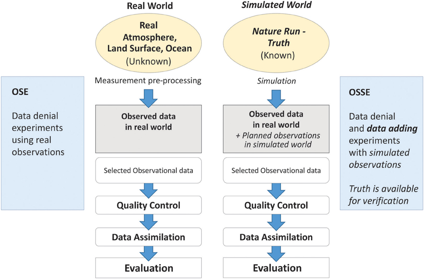
Figure 5. Schematic of an observing system experiment, OSE (left-hand flow diagram), and an observing system simulation experiment, OSSE (right-hand flow diagram). See text for an explanation of the terms in the figure. Based on material in Masutani et al. (2013).

FIGURE 6

Figure 6. Results from an OSSE performed to test the addition of column AOD (aerosol optical depth) measurements from a prospective geostationary (GEO) satellite. Plots use fields of particulate matter of radius less than 2.5 micrometers, PM2.5, units of μgm⁻³, and are averages over the period 25–28 February 2003. The panels show the following. Top row: Nature Run. Second row: left, model run, i.e., without data assimilation; right: difference, model minus Nature runs. Third row, left: assimilation run #1 incorporating synthetic ground-based PM2.5 observations; right: difference, assimilation #1 minus Nature runs. Bottom row, left: assimilation run #2 incorporating synthetic ground-based PM2.5 observations and half-hourly synthetic AOD observations from the proposed GEO satellite; right: difference, assimilation #2 minus Nature runs. In the difference plots, positive values indicate the model or the assimilation values are higher than those of the Nature Run. The model is LOTOS-EUROS, and the assimilation method is the EnKF. With permission from Timmermans et al. (2009b).

The OSSE approach was first adopted in the meteorological community to assess the impact of future observations, i.e., not available from current instruments, in order to test potential improvements in weather forecasting (Nitta, 1975; Atlas, 1997; Lord et al., 1997; Atlas et al., 2003). In a review paper, Arnold and Dey (1986) summarized the early history of OSSEs and presented a description of the OSSE methodology, its capabilities and limitations, and considerations for the design of future experiments. The OSSEs also have been performed to assess trade-offs in the design of observing networks and to test new observing systems (Stoffelen et al., 2006). The recent history of OSSEs, several variants of the OSSE method, and issues concerning their set up and interpretation, and their application, are discussed in Masutani et al. (2010, 2013).

Although OSSEs require significant resources in computing power and human resources, the cost is a small fraction of actual observing systems (Masutani et al., 2013). OSEs can be expensive if they use the full data assimilation system. A more affordable approach to OSEs is provided by the recently developed adjoint-based forecast sensitivity to observations (FSO) technique (Lorenc and Marriott, 2014). Although efficient, the FSO method is limited to evaluating observation impacts on forecasts typically no longer than 24 h due to the necessary approximation of the full forecast model by a simplified linear version. As a result, OSEs still play an important role in evaluating impacts on longer forecasts.

Several OSSEs have been performed to assess the benefit of additions to the GOS to measure winds, either tropospheric winds from ESA's Earth Explorer ADM-Aeolus, the Atmospheric Dynamics Mission (Tan et al., 2007), or stratospheric winds from CSA's⁵ proposed instrument SWIFT, Stratospheric Wind Interferometer For Transport studies (Lahoz et al., 2005). ADM-Aeolus is expected to be launched during mid-2014. As illustrated by their use in ADM-Aeolus, the value of OSSEs is now recognized by the space agencies.

Several OSSEs have been performed to assess the benefit of additions to the GOS to monitor air quality at the surface and lower troposphere (between the surface and ~6 km), notably from GEO platforms. These OSSEs have tended to focus on measurements of ozone and CO (Edwards et al., 2009; Claeyman et al., 2011; Sellitto et al., 2013; Yumimoto, 2013; Hache et al., 2014; Zoogman et al., 2014); ozone is considered because it is a key lower tropospheric pollutant, and CO because it provides information on sources of pollution and transport processes in the lower troposphere. Other OSSEs for air quality have considered measurements of PM, another key tropospheric pollutant (Timmermans et al., 2009a,b). A key aspect of the OSSEs done to assess future observations of ozone and CO to monitor air quality is the recognition of the need for multi-spectral retrievals, typically using combinations including two or more of the thermal infrared (TIR), the visible (VIS) and the ultraviolet (UV) regions of the electromagnetic spectrum (Natraj et al., 2011; Lahoz et al., 2012; Sellitto et al., 2012).

Figure 6 shows the benefit provided by additional observations of column AOD from a GEO. It shows that the experiments incorporating these observations (in addition to ground-based measurements; bottom row of Figure 6) provide the best agreement with the Nature run. By contrast, the model run without assimilation (second row of Figure 6) is not able to reproduce the high levels of pollution seen in the Nature run over The Netherlands and northern Germany. When only ground-based PM2.5 observations are assimilated (third row of Figure 6), the results are closer to the Nature Run than for the model run, but the agreement is not as good as when the satellite data are added.

Given that air quality is a global concern (Lahoz et al., 2012), there are plans for establishing a constellation of GEOs for monitoring air quality in the Northern Hemisphere (CEOS, 2011). More recently, Bowman (2013) discusses the merits of an ozone air quality monitoring system built around a new generation of LEO and GEO satellites, and how it can meet the challenges of air quality and climate. The OSSEs have become a standard tool to assess proposed and planned satellite missions from space agencies in the USA, Europe, and Asia (Tan et al., 2007; CEOS, 2011; Palmer et al., 2011; Lahoz et al., 2012), including those developed for monitoring air quality (Masutani et al., 2013).

Ozone Data Assimilation

Assimilation of ozone in the stratosphere has several objectives. These include: (i) development of ozone and UV-forecasting capabilities; (ii) need to monitor stratospheric ozone to track the evolution of stratospheric composition, mainly ozone and the gases that destroy it, and assess compliance with the Montreal rotocol (WMO, 2006); (iii) need to evaluate the performance of satellite instruments measuring ozone, especially those providing long-term datasets—examples include the TOMS, Total Ozone Mapping Spectrometer, and the GOME, Global Ozone Monitoring Experiment, both providing 2-D total column ozone information; (iv) development of computer code to assimilate instrument radiances sensitive to temperature and constituents; (v) constraints ozone observations provide on other chemical species; (vi) need to evaluate models simulating ozone; and (vii) improving simulations in the stratosphere, chiefly through a better representation of stratospheric winds and temperature as a result of an improved representation of stratospheric ozone.

Assimilation of satellite ozone data, often with a focus on the stratosphere, has been carried out for more than a decade. Examples include: Levelt et al. (1998), Hólm et al. (1999), Khattatov et al. (2000), El Serafy et al. (2002), Struthers et al. (2002), Eskes et al. (2003), Dethof and Hólm (2004), Štajner and Wargan (2004), Massart et al. (2005, 2009), Segers et al. (2005), Wargan et al. (2005, 2010), Geer et al. (2006, 2007), Štajner et al. (2006, 2008), Jackson (2007), Lahoz et al. (2007), Rösevall et al. (2007a,b), Parrington et al. (2008, 2009), Dragani (2011), Sekiyama et al. (2011), Remsberg et al. (2013), and Barré et al. (2014). Assimilation of tropospheric ozone, and other tropospheric pollutants such as NO₂ and PM, has been carried out for air quality purposes: (i) to produce analyses that allow monitoring of pollutant levels and check compliance with legislation (Lahoz et al., 2012); and (ii) to provide the initial state for air quality forecasts (Elbern et al., 2007, 2010; Rouïl et al., 2009).

The main motivation for the inclusion of ozone data assimilation in weather forecasting has been to take better account of ozone when assimilating satellite radiance data, mainly from nadir sounding instruments. Many of the channels used for atmospheric temperature sounding are at least partially sensitive to ozone, so improvements in the accuracy of ozone profiles can lead to more accurate temperature inversions, with benefit to weather forecasting. Work has also taken place to develop the assimilation of radiances sensitive to ozone and humidity from limb-sounding instruments measuring in the infrared (Bormann et al., 2005, 2007; Bormann and Healy, 2006; Bormann and Thépaut, 2007).

The first implementation of an ozone assimilation system for operational weather forecasting was at NCEP (Caplan et al., 1997; Derber et al., 1998). Since then, operational ozone assimilation systems have been developed at various operational centers using GCM- and CTM-based systems. Examples of GCM-based systems include ECMWF (Dragani and Dee, 2008), and the Met Office, UK (Jackson, 2004). Examples of CTM-based systems include the Royal Netherlands Meteorological Institute, KNMI (Eskes et al., 2002, 2005; El Serafy and Kelder, 2003); the Global Modeling Assimilation Office, GMAO (Riishøjgaard et al., 2000; Štajner et al., 2001, 2004); and the Belgian Institute for Space Aeronomy, BIRA-IASB (Viscardy et al., 2010). The GCM and CTM approaches have been combined in coupled data assimilation, e.g., in a collaboration between Environment Canada and BIRA-IASB, where a chemical scheme from BIRA-IASB based on a CTM is coupled to a GCM from Environment Canada (de Grandpré et al., 2009).

Assimilation of ozone observations has provided numerous benefits. (i) Monitoring of satellite ozone observations from time series of observation minus forecast (O-F) differences. (ii) Assessment of error characteristics of observations and models, including quantification of the bias in observations, and whether observational and model errors are consistent with the assumption of a Gaussian PDF by checking if O-F differences have a Gaussian PDF—if the observations and the forecast have Gaussian PDFs, O-F differences should also have a Gaussian PDF. (iii) Evaluation of ozone satellite observations using an ozone analysis to interpolate in space and time between the satellite observations and independent data used for the evaluation (independent data being data not used in the assimilation), either from satellite or in situ observations. (iv) Assessment of the impact of new observations on the representation of ozone distributions. (v) Assessment of the relative performance of the complexity of model representations of ozone chemistry, e.g., a comparison between a parametrization of the sources and sinks of ozone and a detailed photochemical scheme, including heterogeneous reactions. (vi) Assessment of various parametrizations of the sources and sinks of ozone. Further details can be found in Lahoz and Errera (2010) and references therein.

Figure 7 provides details of a comparison of ozone data assimilation systems with varying complexity in the way they represent ozone photochemistry (Geer et al., 2006). The comparison is for 18 August–30 November 2003, and includes the period of the Antarctic ozone hole, when there is significant ozone loss in the stratosphere, challenging for the data assimilation systems. The assimilation systems are compared for the same atmospheric conditions. Figure 7 shows that in the stratosphere (100–10 hPa), and for situations where the density and quality of ozone observations is high, the complexity of the ozone photochemistry representation does not have large impact on the quality of the ozone analysis. This result informs efforts to develop data assimilation methods to assimilate stratospheric ozone, whether for research or for operational (e.g., weather forecasting) purposes.

FIGURE 7

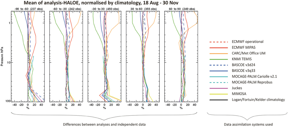
Figure 7. Left section (5 panels): mean of ozone analyses minus ozone data from the HALOE (Halogen Occultation Experiment) instrument, normalized by climatology, and shown as a percentage of the climatology. The period considered is 18 August–30 November 2003 and five latitude bins are represented in the panels. Right section (legend): color key for the plots on the left, indicating the data assimilation systems used, themselves varying in complexity, and for comparison, an ozone climatology from Fortuin and Kelder (1998). Based on material in Geer et al. (2006).

Land Surface Data Assimilation

Assimilation of land surface observations is at an earlier stage than, e.g., assimilation of atmospheric observations (Lahoz et al., 2010b). However, during the past decade, land surface data assimilation has been a very active field of research. Land surface data assimilation considers both ground-based in situ data and satellite data. Often, satellite land surface data are assimilated and the process validated using in situ measurements. Three methods are commonly used for land surface data assimilation (Houser et al., 2010): variational (3D- and 4D-Var); sequential (KF and EKF); and ensemble (EnKF). The data assimilation research applications for the land surface consider: (i) single column applications, concerning single point-scale, or grid cell-scale applications; and (ii) distributed applications, concerning relatively large scales (although for computational reasons this is often performed per column, using a 1-D filter). Operational assimilation for the land surface is discussed by de Rosnay et al. (2014). Assimilated satellite observations include retrievals of land surface temperature (e.g., Ghent et al., 2010), soil moisture (e.g., Reichle and Koster, 2005), snow water equivalent (SWE) (e.g., De Lannoy et al., 2010), and snow cover area (e.g., De Lannoy et al., 2012). Parameter estimation is also performed (e.g., Pauwels et al., 2009; Vrugt et al., 2012). Lahoz and De Lannoy (2014) provide comprehensive references describing the assimilation of land surface observations, including retrievals and radiances.

Soil moisture is a key geophysical variable for understanding the Earth's hydrological cycle. It is classed as an ECV of the GCOS. Soil moisture determines the partitioning of incoming water into infiltration and run-off. It directly affects plant growth and other organic processes, connecting the water cycle to the carbon cycle. Run-off and base flow from the soil profile determine river flows and flooding, connecting hydrology with hydraulics. Soil moisture also has a significant impact on the partitioning of water and heat fluxes (latent and sensible heat), connecting the water cycle with the energy cycle. More details on the role of soil moisture in the Earth System can be found in Seneviratne et al. (2010).

Integration of soil moisture information from various observational platforms, using land surface data assimilation, provides a comprehensive picture of the state and variability of the land surface. However, large differences in the spatio-temporal resolution of satellite and in situ soil moisture measurements (i.e., retrievals); the different depth of penetration of soil moisture information from satellite platforms—ranging from a few mm for the X-band (8–12 GHz) for the AMSR-E (Advanced Microwave Scanning Radiometer—Earth Observing System) satellite, to ~1 cm for the C-band (4–8 GHz) for the ASCAT (Advanced SCATterometer) satellite, and ~5 cm for the L-band (1–2 GHz) for the SMOS (Soil Moisture and Ocean Salinity) satellite; the larger depth of penetration for in situ soil moisture platforms, typically ~10 cm and deeper (see information provided by the ISMN, International Soil Moisture Network⁶); and differences in the techniques of satellite measurements (active and passive remote sensing), make it challenging to use satellite and in situ observations of soil moisture in a land surface data assimilation system. The land surface also exhibits features which make applying data assimilation algorithms challenging: heterogeneity (spatial scales are much smaller than for the atmosphere and the ocean); non-linearities and on-off processes (e.g., presence or lack of snow); and elements which exhibit non-Gaussianity (e.g., the hydrological cycle). The non-linear and non-Gaussian features of the land surface make data assimilation methods such as the PF attractive (see section Representation of Errors).

Land surface data assimilation has a number of challenges, and many concern general applications of data assimilation (see section Challenges in Data Assimilation). The latter include: (i) need to assimilate radiances to avoid inconsistencies between the prior information used in the retrieval and in the data assimilation (Crow and Wood, 2003; Durand et al., 2009; Flores et al., 2012); (ii) need to exploit multiple sensors (Pan et al., 2008; Draper et al., 2012), and explore capabilities of new sensors (Andreadis et al., 2007; Durand et al., 2008); (iii) need to combine state and input (forcing) information with parameter updates (Moradkhani et al., 2005b; Liu et al., 2011; Vrugt et al., 2012); (iv) need to improve representation of observational and model errors, and specify biases in the observational and model information (De Lannoy et al., 2007b; Crow and Reichle, 2008; Reichle et al., 2008; De Lannoy et al., 2009; Crow and van den Berg, 2010); and (v) need to have adequate computer resources. Challenges particular to the land surface include: (i) need to explore advanced data assimilation methods such as the PF (see section Representation of Errors); and (ii) need to preserve water balance in the land system (Pan and Wood, 2006; Yilmaz et al., 2011).

Figure 8 shows an example of the assimilation of AMSR-E and MODIS (MODerate resolution Imaging Spectroradiometer) snow observations for one snow season in Northern Colorado, USA (De Lannoy et al., 2012). AMSR-E retrievals are coarse-scale (25 km) SWE estimates, with data missing when the swath does not cover the study area. To estimate the snow at a fine model scale (1 km), an EnKF is applied. This allows: (i) downscaling coarse-scale observations to the fine scale; and (ii) propagating observed observations to unobserved areas, thus enabling smooth fine-scale SWE estimates. This illustrates two benefits from the data assimilation method. MODIS provides fine-scale estimates of snow cover fraction (SCF), but only over cloud-free areas. To assimilate this indirect snow information, a snow depletion curve acts as the observation operator converting modeled SWE into SCF estimates. Unlike binary (non-continuous) indicators of snow presence, the continuous SCF observations can be assimilated with an EnKF, except for snow-free or full cover conditions. These latter conditions are treated by supplementing the EnKF with a rule-based update.

FIGURE 8

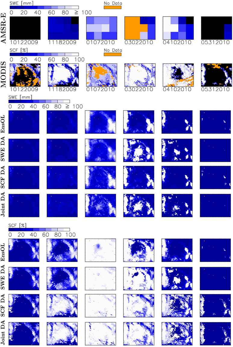
Figure 8. Snow water equivalent, SWE (at 08:00 UTC) and snow cover fraction, SCF (at 17:00 UTC) fields for 5 days (MMDDYYYY) in the winter of 2009–2010. No snow is indicated as black. The top 2 rows show individual SWE and SCF satellite observations. The remaining rows show SWE (at 09:00 UTC—block of middle four rows) and SCF (at 18:00 UTC—block of bottom four rows) for the Ensemble Open Loop (EnsOL) forecast, i.e., not using assimilation and three different analyses obtained through data assimilation (DA) without a priori scaling: SWE DA, SCF DA and joint SWE-SCF DA, respectively. AMSR-E data are missing due to the swath effect and MODIS data are missing because of cloud cover. With permission from De Lannoy et al. (2012).

The realism of the SWE patterns shown in Figure 8 from joint assimilation of coarse-scale AMSR-E SWE and fine-scale MODIS SCF observations can be inferred from evaluation of the SWE analyses against independent snow data from in situ observations at high-elevation Snowpack Telemetry (SNOTEL) sites with typically deep snow and at lower-elevation Cooperative Observer Program (COOP) sites (see De Lannoy et al., 2012). This reinforces the need to evaluate analyses produced by data assimilation against independent data, i.e., data not used in the assimilation procedure (see Figure 2).

Other Applications of Data Assimilation

Besides examples illustrated in sections Observing System Simulation Experiments for Monitoring Air Quality–Land Surface Data Assimilation, data assimilation is also applied in other areas by operational centers such as ECMWF, and by research centers. We discuss below the following areas: atmospheric chemistry; the ocean, including waves; and reanalyses.

Atmospheric chemistry

Early examples of the methods used in chemical data assimilation include nudging (Austin, 1992); variational methods (Fisher and Lary, 1995); and sequential methods based on variants of the KF (Khattatov et al., 1999). More recently, ensemble methods have been developed for chemical data assimilation (Constantinescu et al., 2007b,c).

Following on from these efforts, chemical data assimilation has been used to test chemical theories (Lary et al., 2003; Marchand et al., 2003, 2004); study transport processes (Cathala et al., 2003; Semane et al., 2007; Barret et al., 2008; El Amraoui et al., 2008; Barré et al., 2012, 2013); extract wind information from constituent information (Riishøjgaard, 1996; Hólm et al., 1999; Peuch et al., 2000; Semane et al., 2009); produce analyses of chemical species, including ozone, NO₂, NO_x (NO+NO₂), CH₄, N₂O, CO, CO₂, water vapor and aerosols (Fonteyn et al., 2000; Ménard and Chang, 2000; Ménard et al., 2000; Errera and Fonteyn, 2001; Chipperfield et al., 2002; El Amraoui et al., 2004; Arellano et al., 2007; Errera et al., 2008; Chai et al., 2009; Engelen et al., 2009; Tangborn et al., 2009; Thornton et al., 2009; Miyazaki et al., 2012, 2014; Miyazaki and Eskes, 2013—for a representative list of references for ozone see section Ozone Data Assimilation); and design constituent measurement strategies (Khattatov et al., 2001). There have been efforts to improve the chemical data assimilation methodology, including representation of the background errors (Constantinescu et al., 2007a; Singh et al., 2011; Errera and Ménard, 2012); assessment of technical aspects of the chemical model, e.g., adjoint sensitivity (Sandu et al., 2003, 2005); and comparison of assimilation methods, e.g., 4D-Var vs. EnKF (Skachko et al., 2014). Reviews of chemical data assimilation include those by Lary (1999), Wang et al. (2001), Khattatov (2003), Lahoz et al. (2007), and Sandu and Chai (2011).

Chemical data assimilation is increasingly being used for research on tropospheric pollution and air quality. The steps toward this work have included the demonstration that data assimilation can improve analyses of tropospheric pollution (Elbern and Schmidt, 2001), and that inverse modeling can provide estimates of tropospheric emissions like CO (Müller and Stavrakou, 2005) or CH₄ (Meirink et al., 2006). More generally, it has been shown that inferring sources and sinks of constituents using inverse modeling provides information on transcontinental pollution (e.g., Pétron et al., 2004), air quality (e.g., Blond and Vautard, 2004), and national greenhouse gas inventories (e.g., Bergamaschi et al., 2005).

Nowadays, with the availability of atmospheric composition measurements from various satellite platforms, e.g., ESA's Envisat (launched in 2002), NASA's EOS Aura (launched in 2004), and JAXA's GOSAT (launched in 2009)⁷, it has become possible to replicate results from weather forecasting by providing forecasts and analyses of atmospheric constituents based on chemical models and data assimilation techniques. The EU-funded project Monitoring Atmospheric Composition and Climate Interim Implementation (MACC-II⁸), and its predecessors GEMS (Global Earth system Monitoring using Space and in situ data) and MACC, have led the way in these activities toward implementing the operational atmospheric service of Copernicus⁹. A recent example of the work in MACC is the assimilation of methane (CH₄) data (Massart et al., 2014).

A further application of data assimilation to atmospheric chemistry is combined state estimation and inverse modeling, where it is used to both estimate the system state and the emissions or fluxes. This is done by extending the state x in Equation (2) to include emissions/fluxes—in the case of parameter estimation, x is extended to include, e.g., model parameters. The system state is analogous to the initial conditions for a forecast, and the emissions/fluxes are analogous to the sources and sinks in the system. This approach, as applied to atmospheric constituents, is discussed in Elbern et al. (2010).

The data assimilation approach is also applied to the main biogeochemical cycles in the Earth System: the carbon cycle, to estimate model parameters (e.g., Rayner, 2010), and CO₂ fluxes (e.g., Peylin et al., 2013); and the nitrogen cycle, to estimate N₂O fluxes (e.g., Thompson et al., 2014). It is also applied to estimate fluxes of CH₄ (e.g., Bergamaschi et al., 2009; Bousquet et al., 2011). These species considered (CO₂, N₂O, and CH₄) are important greenhouse gases in the Earth System.

Ocean, including waves

A major application of ocean data assimilation is extended range forecasts (seasonal and monthly) at weather centers across the world, including ECMWF (Stockdale et al., 1998), NCEP (Barnston et al., 1999), and the Japanese Meteorological Agency, JMA (Ishii et al., 1998). Ocean reanalyses are routinely produced at the weather centers, particularly for initializing the ocean as part of dynamical seasonal forecast systems. The ECMWF seasonal and monthly forecasting systems¹⁰ are illustrative of the approach to ocean assimilation; they are based on a coupled ocean-atmosphere GCM that predicts both the lower boundary conditions (sea surface temperatures) and their impact on the atmospheric circulation. The various phenomena in the ocean have a wide range of spatio-temporal scales and this has to be accounted for in the design of ocean assimilation systems.

The current ECMWF operational ocean analysis system is Ocean-S4. It consists of two analysis streams: (i) a historical reanalysis from 1957 to the present¹¹, used to initialize the coupled hindcasts needed for calibration of coupled model output—this is ORA-S4 (Ocean ReAnalysis System 4); and (ii) a daily real time ocean analysis¹², used to initialize the coupled forecasts—this is ORT-S4 (Ocean Real Time System 4). The Ocean-S4 system is based on the NEMO (Nucleus for European Modeling of the Ocean) model (Madec and the NEMO Team, 2008) and on the NEMOVAR data assimilation system (Mogensen et al., 2012). Daily surface fluxes of heat, momentum and fresh water are used to force the ocean model and to produce the first guess of the state of the ocean.

The NEMOVAR assimilation system is used to assimilate temperature and salinity (T/S) profiles as well as along track altimeter derived sea level anomalies. The T/S profiles come from several data types, including XBTs—expendable bathythermographs (temperature only); and CTDs—conductivity temperature depth instruments, moorings, Argo profilers, and elephant seals (temperature and salinity). The sea level anomalies come from the AVISO (Archiving Validation and Interpretation of Satellite Oceanographic data) system¹³. A bias correction scheme is used to correct the model/forcing errors. The bias correction is needed to reduce spurious variability that can arise from changes in the observing system. Details of how altimeter satellite data and in situ T/S data are assimilated into ocean systems can be found in Haines (2010).

At ECMWF a range of products forecasting the sea state is provided by an ocean wave forecast model¹⁴. This model is directly coupled to the atmospheric model: the ocean waves are driven by low-level atmospheric winds, and in turn the roughness of the sea determines how much the air is slowed down as it flows over the ocean surface. This coupled wave model forms part of the ensemble prediction system, providing probabilistic information on future sea states.

Other European centers involved in ocean assimilation include the Met Office, UK¹⁵; and the Nansen Environmental and Remote Sensing Center, NERSC, Norway¹⁶. The Met Office system provides a sea surface temperature analysis product¹⁷ that is used for a wide range of applications, including NWP and climate monitoring. The TOPAZ-4 system from NERSC is an operational coupled ocean-sea ice data assimilation system for the North Atlantic Ocean and Arctic (Sakov et al., 2012a).

USA centers involved in ocean assimilation include NCEP, GMAO, and GFDL (Geophysical Fluid Dynamics Laboratory). NCEP developed GODAS, the Global Ocean Data Assimilation System (Behringer and Xue, 2004). It produces real-time ocean analyses and reanalyses for monitoring, providing retrospective analyses, and providing ocean initial conditions for the CFS (Climate Forecast System) at NCEP. GMAO developed GEOS iODAS¹⁸ (Vernieres et al., 2012). It is implemented within the GEOS-5 modeling system under the Earth System Modeling Framework (ESMF). GEOS iODAS can be used either in ocean only integrations or in coupled model experiments with any ESMF compatible ocean and atmospheric model. The main goal of the Ocean Data Assimilation Experiment at GFDL¹⁹ is to develop a state-of-the-art assimilation system that incorporates near-real time ocean data to provide the community a high quality ocean state product.

Another ocean assimilation effort is that of ECCO (Estimating the Circulation and Climate of the Ocean²⁰). ECCO was established in 1998 as part of the World Ocean Circulation Experiment (WOCE) with the goal of combining a GCM with diverse observations to quantify the time-evolving global ocean state. The importance of this effort is recognized by numerous national and international organizations, including the WMO's World Climate Research Programme (WCRP) and UNESCO's Intergovernmental Oceanographic Commission (IOC). These programs have recognized the need of synthesizing the remotely-sensed and in situ observations of the ocean with known dynamics and thermodynamics through a GCM. ECCO products support the Climate Variability and Predictability (CLIVAR²¹) programme and the Global Ocean Data Assimilation Experiment (GODAE²²).

Reanalyses

Reanalyses are performed to provide self-consistent information on the Earth System to monitor the climate, and help understand the predictability of weather patterns (Rood and Bosilovich, 2010). Examples include reanalyses of the atmosphere and atmospheric composition, ocean and land surface.

The ECMWF carried out the first reanalysis of the global land-surface and atmosphere in the early 1980s for the First GARP Global Experiment (FGGE) year (1979), when ECMWF operations began. This was followed by two major reanalyses that exploited substantial advances made in the ECMWF forecasting system and technical infrastructure. The first reanalysis, ERA-15 (1979–1993, ERA—ECMWF ReAnalysis), was completed in 1995, and the second reanalysis, ERA-40 (1957–2002), in 2002. Products from ERA-15 and ERA-40 (Uppala et al., 2005) have been used extensively by the operational and scientific communities, and by the wider user community. Today, ECMWF is producing the ERA-Interim reanalysis²³, which covers the data-rich period since 1979. The ERA-Interim data assimilation system uses a 2006 version of the Integrated Forecasting System (IFS), which contains many improvements both in the forecasting model and analysis methodology relative to ERA-40. The ERA-Interim reanalysis caught up with real-time in March 2009 and has continued in near-real time to support climate monitoring. The ECMWF has also produced a pilot reanalysis assimilating only surface pressure observations for the time period 1899–2010. A similar reanalysis, spanning 1871–2011, has been done in the USA—the Twentieth Century Reanalysis Project (Compo et al., 2011).

The ECMWF has produced a global reanalysis that includes atmospheric composition within the MACC and MACC-II projects. The data assimilation method used in the MACC reanalysis is incremental 4D-Var (Inness et al., 2013). The MACC reanalysis covers a 10 year period, from January 2003 to December 2012 and covers aerosols, reactive gases, and greenhouse gases. The MACC reanalysis combines state-of-the-art atmospheric modeling with Earth Observation data providing a fully consistent meteorological and atmospheric composition dataset.

The ECMWF produced the first ocean reanalysis in 1996, when it started running the first seasonal system (S1). Today, ECMWF is producing a global ocean reanalysis with ORA-S4, which covers the period from 1958 to the present. The ECMWF ocean reanalyses (from the first one, ORA-S1, to the latest one, ORA-S4) are widely used by the research community, including the climate community in the initialization of decadal forecasts. Implementation of the ocean reanalyses at ECMWF is a prime example of how reanalyses can be exploited as an integral part of a coupled forecasting system.

Outlook

Recent Developments

The major science challenges for the weather centers at the start of the Twenty-first Century include²⁴: (i) forecasting hazardous weather (e.g., storms) at temporal scales from hours to decades; (ii) forecasting the hydrological cycle and rainfall at all spatio-temporal scales; (iii) forecasting at monthly, seasonal, interannual, and decadal temporal scales in a changing climate; and (iv) understanding, assessing, and monitoring the sensitivity of the Earth System to human activities. Addressing these challenges requires that weather centers, and other institutions involved in data assimilation research (climate centers, academia), investigate a number of key areas in data assimilation. These include the representation of observational and model errors; inclusion of various elements of the Earth System, and the two-way interactions between them; a reduction in the spatial scales being considered for forecasts; and an extension of the GOS to include novel observational platforms.

The weather centers are at the forefront of efforts to improve on the representation of errors in observational and model information used in data assimilation (section Data Assimilation Methodology). Recent developments include combination of ensemble and variational methods to describe the background errors used to represent uncertainty in prior knowledge (B matrix introduced and discussed in section Variational Methods). This involves developing hybrid covariance models, e.g., a linear combination of a static B matrix (built from climatology and typically used in 4D-Var applications) with a flow-dependent B matrix (described using an ensemble). Such a hybrid approach has been operational at ECMWF for some time (Buizza et al., 2008; Isaksen et al., 2010; Bonavita et al., 2012), and is now operational at the Met Office, UK, for the global model (Clayton et al., 2013) and at Environment Canada (Buehner et al., 2010). A theoretical basis for the construction of the hybrid covariances, in particular how to weight the static and flow-dependent components, can be found in Bishop and Satterfield (2013) and Bishop et al. (2013).

The broad ensemble-variational approach (EnVar), which uses ensemble information throughout the data assimilation time window and a variational minimization step to find the optimal analysis, is described in Fairbairn et al. (2014). A benefit of EnVar is the cheaper minimization of the cost function due to a linear and adjoint model not being required to propagate covariance information throughout the window, as is needed in 4D-Var. The non-linear propagation of the covariance information by the ensembles may also include a better representation of non-Gaussian behavior. The requirement not to have a linear and adjoint model allows the approach to be adaptable to a range of model grids.

Assimilation of radiances and retrievals is also an area of research at weather centers. For example, the EUMETSAT NWP SAF (Satellite Application Facility) are developing observation operators for some satellite measurements, e.g., RTTOV, and ROPP²⁵, for assimilation into NWP models.

Developments in Earth System models at weather centers also focus on including various elements of the Earth System, and taking account of their two-way interactions. As a result, an integrated strategy is being implemented at ECMWF, in which various elements of the Earth System are coupled using ensemble methods to produce ensemble coupled analyses and reanalyses (Buizza, 2013). Developments toward ensembles of coupled analyses and reanalyses at the weather centers rely on research which is expected to improve models by: (i) improving the design of simulated processes; (ii) including missing processes, e.g., sea-ice and ocean wave-current interactions; (iii) simulating model uncertainty and sub-grid scale processes; (iv) taking fuller account of external forcings; and (v) initializing in an accurate way all model components, including the atmosphere, ocean and land surface.

The above developments should improve data assimilation efforts at the weather centers through use of better models, with consequent improvement in the accuracy of weather forecasts, and other applications of data assimilation (section Applications of Data Assimilation). The notion that predictability can be considered as a seamless weather-climate prediction problem, and that there can be predictive power on all temporal scales (Palmer et al., 2008; Hoskins, 2013) allows a two-way process where correction of errors at longer time-scales (appropriate to climate processes) leads to improvements at shorter time-scales (appropriate to weather processes), and viceversa. An example of this approach is provided by Rodwell and Palmer (2007), who discuss the use of NWP to assess climate models.

In reanalyses (section Other Applications of Data Assimilation), recent developments at weather centers involve maintaining and improving atmospheric and ocean reanalyses, many applying EnKF techniques that produce ensembles of analyses²⁶. These reanalyses are becoming increasingly important for climate studies and for reforecast initialization (reforecasts are used for statistical post-processing)—e.g., Balmaseda et al. (2013) use the ECMWF ocean reanalysis ORA-S4 to help explain the so-called climate warming hiatus of the past decade. The Japanese 55-year reanalysis has just been completed²⁷. The EnKF-based Twentieth Century reanalysis is now available (Compo et al., 2011). The ECMWF continues to run the ERA-Interim reanalyses, with future reanalyses planned. There are also several regional reanalyses activities underway.

Another recent development in data assimilation at weather centers concerns moves toward higher resolution modeling, involving smaller spatial scales, typically 100 s of meters. A particular interest of moving toward smaller spatial scales is performing data assimilation at convective scales. These smaller spatial scales are closer to the needs of users than the scales used hitherto in data assimilation applications, including those from weather centers. The increased emphasis on higher resolution modeling is one pillar of the Met Office strategy for 2010–2015²⁸, which also includes a focus on research into processes and phenomena in the Earth System, and an enhanced use of Earth Observation.

The Sixth WMO Data Assimilation Symposium (see Applications of data assimilation) provided a snapshot of current developments in data assimilation, and how they reflect the key areas mentioned above: representation of errors; inclusion of various elements of the Earth System; a reduction of spatial scales; and extension of observational platforms. The accuracy of modern weather forecasting systems continues to improve, and accurate forecasts of mid-latitude storms and tropical cyclones up to 7 days ahead are now common. Key contributions to this achievement are advances made in data assimilation, coupled with increased computer power, better weather prediction systems, and more extensive observing systems (see Simmons and Hollingsworth, 2002). Experiments with reanalyses have shown that data assimilation systems (and the improved forecast models they use for the background) are a primary source of the improved forecast accuracy.

Themes at the Sixth WMO Data Assimilation Symposium included: data assimilation methods (weak-constraint 4D-Var; variants of the EnKF; hybrid methods to represent background errors); data assimilation diagnostics (OSEs; OSSEs; FSOs); data assimilation for the Earth System, including coupling and reanalyses (atmosphere-ocean; atmosphere-land surface); improved use of observations (radar reflectivity; atmospheric motion vectors); and consideration of smaller spatial scales (e.g., convective scales). All the abstracts, slides and, for most sessions, webinar recordings from the symposium are available at http://das6.cscamm.umd.edu/. This is a valuable resource for the data assimilation community.

Challenges in Data Assimilation

Among the technical challenges in data assimilation, a number are significant. These are: (i) coherent coupled assimilation of data between different elements of the Earth System—examples include coupling of transport and chemical information, and coupling of the atmosphere and the ocean, and of the atmosphere and the land surface; (ii) performing data assimilation at increasingly smaller spatial resolutions (mesoscale and finer scales), including theoretical developments to account for changes in balance conditions; (iii) better representation of errors in the observations and models used in data assimilation, including representation of forecast errors and model errors, and implementation of on-line bias corrections; and (iv) extension and consolidation of the joint state estimation and the inverse modeling approach to study biogeochemical cycles (e.g., carbon and nitrogen cycles).

A main challenge in data assimilation for the weather centers concerns its implementation at the convective scale. Smaller spatial scales such as convective scales have challenges, both in the treatment of observational information (e.g., characterizing errors of representativeness), and of model information (e.g., characterizing small-scale processes hitherto treated using parametrizations representing their impact at larger scales). It is not clear whether variational methods will be applicable—the problem is too non-linear, and perhaps only ensemble methods can be used. Convective scale forecasts are in high demand by national governments to provide detailed hazardous weather warnings. For example, the Met Office has a Nowcasting Demonstration Project which ran a 300 m resolution model over the south of England with 4D-Var for several months, including the period of the 2012 summer floods (June-August) and the 2012 London Summer Olympics, held in July–August (Ballard et al., 2013). Another big challenge for convective scale models is proper handling of the effects of the boundary conditions provided by a global model.

There are a number of further challenges on which weather centers such as ECMWF are working on. These include: (i) scalability of data assimilation algorithms (e.g., development of parallelization techniques with ensembles); (ii) accommodation to increased data volumes (e.g., currently, ECMWF only uses ~10% of the satellite data received); (iii) validity of assumptions of linearity in the observation and model operators (see sections Variational Methods–Sequential Methods) and of Gaussianity in the observational and model information (e.g., for convective scales); and (iv) coupled assimilation (e.g., dealing with Earth System elements having different temporal scales).

The overarching challenge for data assimilation is the consolidation and integration of community efforts in the extraction of information from various observational platforms, and the effective application of these efforts toward development of new missions in Earth Observation. A new challenge is the exploitation of observational platforms based on Citizen Science, discussed in sections Citizen Science–Data Assimilation and Citizen Science. The benefits of addressing these challenges in data assimilation are likely to include improvements to weather forecasting; improvements to reanalyses; an improved observational system; and an improved foundation on which the elements of climate models can be built (see, e.g., Gimeno, 2013).

As shown in section Applications of Data Assimilation, the data assimilation method is not just weather-centric, but applies elsewhere, with insights from the work of the weather centers being helpful. Newer applications, e.g., in the area of Citizen Science, can benefit and/or leverage from issues known in already established fields, and viceversa.

Citizen Science

In the EU, several new Citizen Science initiatives funded by the Seventh Framework Programme for Research are underway (Science Communications Unit, 2013). These explore the potential of Citizen Science to provide information on the environment (e.g., air quality, meteorological conditions), and inform environmental policymaking. As part of the EU activities regarding Citizen Science, the SOCIENTIZE consortium²⁹ is co-ordinating an ongoing public consultation and debate about the potential role of Citizen Science in Europe. In an intermediate step, the SOCIENTIZE consortium has produced a Green Paper³⁰ which presents the major themes and some of the recommendations that will be refined in a White Paper on Citizen Science planned for 2014. These major themes are: (i) definition and scope of Citizen Science; (ii) deployment, facilitation, and sustainability for Citizen Science activities at local, national, and European levels; (iii) awareness and motivation for active involvement of citizens; (iv) drivers and barriers for Citizen Science; (v) impact measurement and evaluation of Citizen Science; and (vi) the emerging public debate on efficiency and excellence in science. The recommendations are at policy level, science and technology level, and society level; they involve actions to bring forward the major themes (i)–(vi) above, and provide the basis for the successful application of Citizen Science to the benefit of the European citizen.

A concept associated with Citizen Science is that of the Citizen's Observatories (Science Communications Unit, 2013). The Citizen's Observatories consist of communities of users that share technological solutions, information products and services, and community participatory governance methods using appropriate communication solutions, and who by these activities complement established environmental data and information systems and improve local decision making about environmental issues. The Citizen's Observatories concept is closely linked to the notion of “crowdsourcing” (Howe, 2010). When “crowdsourcing” is used to obtain observations about, for example, an environmental parameter it is often referred to as “participatory sensing.” An attractive feature of the Citizen's Observatories is their potential to extend and/or complement the information from established observational platforms (in situ and satellite data).

The Citizen's Observatories concept is built on the fact that smartphones are becoming increasingly ubiquitous, given growth in mobile use, changes in mobile usage, and the increasing range of features provided to mobile phone users. Through a smartphone, the citizen can provide and receive information on their immediate environment (Lahoz, 2013), e.g., at the most basic level using only the phone's internal sensors on temperature, noise, movement, location, or on a wide variety of other parameters using external sensor packs. This includes air quality parameters such as NO_x, CO, ozone, and PM, which can be measured by deploying small, low-cost external microsensors, and using the smartphone as the main communications device. In addition, smartphones allow users to easily submit geo-located observations on nearly any generic parameter using specific apps—a concept called Volunteered Geographic Information (VGI).

Ongoing work at the Met Office (Weather Observations Website, WOW³¹) makes use of the concept of crowdsourcing to obtain information on various meteorological parameters (temperature, rainfall rate, and snowfall) in the UK. The WOW concept is taking off in other countries now, e.g., in Australia. A point to note is that snow depth, a popular thing to measure by UK citizens and broadcast in WOW, is a quantity difficult to measure with an automated system. In this respect, crowdsourcing activities at WOW regarding snow depth provide a valuable observational platform for weather centers. Other crowdsourcing activities planned at the Met Office include the use of solar cell observations on citizen's roofs to measure cloud; a small project has been started to demonstrate the feasibility of this approach. Crowdsourcing is also being used to provide temperatures in an urban environment using solely the internal battery temperature sensors of smartphones (Overeem et al., 2013). Other examples of crowdsourcing can be found in Science Communications Unit (2013).

The use of Citizen Science for data assimilation brings its own challenges. These include: significantly different spatial scales compared to those at which data assimilation is traditionally performed (10–100 km vs. street level, i.e., 10–100 s of meters)—see Figure 9; model development (the need to simulate smaller spatial scales); noisy information from users and from microsensors (Shanley et al., 2013); and representation of uncertainty in a way that is user-friendly and informative (Spiegelhalter et al., 2011). A further challenge is the merging of data from traditional sources such as satellite and in situ platforms, and data provided by Citizen Science. These technical challenges are being addressed in the EU-funded CITI-SENSE project³², which will study a number of approaches to provide gridded air quality and meteorological data for users, including one or more of data assimilation (Lahoz et al., 2010b), data fusion (Warner et al., 2014), and land-use regression (Ryan and LeMasters, 2007; Wen et al., 2013). Notable challenges associated with Citizen Science activities using smartphones that also need to be addressed include quality of data from low-cost sensors, and concerns about data security and data privacy.

FIGURE 9

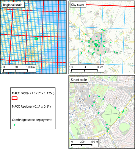
Figure 9. Illustration of significant differences in spatial scale between operational atmospheric modeling and typical data assimilation applications (case 1); and urban air quality applications (case 2). Spatial scales associated with case 1 are exemplified by the global and regional grids used by the MACC-II project as a precursor of the Copernicus Atmospheric Monitoring Service—top left-hand panel (labeled regional scale). Spatial scales associated with case 2 are exemplified by the observations of gases relevant for urban air quality (CO, NO, and NO₂) collected by low-cost, high-density monitoring networks by the University of Cambridge—top right-hand panel (labeled city scale), and bottom right-hand panel (labeled street scale). Spatial resolutions of the global and regional scale MACC models identified in the top two panels are, respectively, 1.125° × 1.125° and 0.1° × 0.1°. The University of Cambridge data are described in Mead et al. (2013).

A further challenge associated with the use of Citizen Science information, and Earth System information in general, is data policy, in particular the issue of “open data” access. A question is whether the citizen is entitled to free access to all data collected by state-funded organizations (i.e., public sector information), especially as one can argue they have already paid for this data through their taxes. These issues are being discussed in the digital agenda for Europe³³. In this context “open data” refers to the idea that certain data should be freely available for use and re-use. The European Commission's work in the area of open data focuses on generating value through re-use of a specific type of data, namely, public sector information, sometimes also referred to as government data. Examples of these data include: geographical information; statistics produced by data manipulation; weather data; data from publicly funded research projects, and digitized books from libraries. The European Commission supports open data for the following reasons: (i) public data has significant potential for re-use in new products and services; (ii) having more data openly available helps address societal challenges, and discover innovative solutions; (iii) sharing data within and between public sectors makes for efficient use of these data; and (iv) it fosters participation of citizens in political and social life, and increases government transparency.

Data Assimilation and Citizen Science

Within the EU-funded CITI-SENSE project, several European cities, spanning various climate regions from the Mediterranean to Scandinavia, are planning to develop networks of both static and portable, low-cost microsensors to monitor local air quality, as well as meteorological parameters. These networks will provide Citizen Science information. As an example of the expected observations, a network to be deployed throughout the city of Oslo, Norway, will consist of 40 static nodes with air quality sensors and associated communication equipment. Each node will measure the concentrations of NO, NO₂, SO₂, O₃, CO, as well as meteorological parameters such as air temperature, relative humidity, and atmospheric pressure in 15 min intervals and automatically upload the information to a server for further processing.

Observations collected by Citizen Science methods such as those from microsensors and smartphones, are usually sampled irregularly in space and time; generally contain large amounts of questionable measurements; and often exhibit significant data gaps. Furthermore, these observations are usually associated with substantial uncertainties. Nonetheless, one of the primary objectives for using such data is to provide citizens with spatially continuous maps of air quality at spatio-temporal scales relevant to them (e.g., 10–100 s of meters, and 1 h or less). It is therefore necessary to map the data in an intelligent way while at the same time accounting for their shortcomings.

In this context, several approaches of increasing complexity are being evaluated for providing users with gridded fields and for investigating the feasibility of using data assimilation techniques (and data fusion as a subset) with observations acquired by Citizen Science. The most basic approach involves very simple interpolation techniques, such as inverse distance weighting and related methods. A second approach involves geostatistical techniques (Goovaerts, 1997; Wackernagel, 2003), which use a theoretical semi-variogram for modeling the spatial autocorrelation of the data and apply it to provide the BLUE of the prediction variable, with the additional option of using independent and spatially distributed auxiliary variables, for example for implementing land-use regression models. Such data fusion techniques can be automated relatively easily and, therefore, can be implemented in an operational system to provide gridded fields of air quality parameters based on observations collected using Citizen Science.

A third approach, data assimilation, is more complex than the two approaches mentioned above, but is by far the most versatile of these three approaches. As an example, within the CITI-SENSE project, an EnKF approach (section Ensemble Methods) is being evaluated for assimilation of air quality observations from Citizen Science into a state-of-the-art high-resolution air quality model, EPISODE (Slørdal et al., 2003), to provide objective interpolated fields.

To illustrate the type of model required to address spatio-temporal scales involved in Citizen Science for air quality purposes, the EPISODE model is a three-dimensional (3-D), combined Eulerian/Lagrangian air pollution dispersion model that has been developed with a main focus on urban and local-to-regional scale applications. The EPISODE model provides gridded fields of ground-level average concentrations of chemical species at a horizontal spatial resolution ranging from 100 m to 10 km and a time step between 10 and 300 s. The model includes schemes for advection, turbulence, deposition, and chemistry. Issues to be addressed in the application of data assimilation to Citizen Science include representation of observational and model errors (taking account of the smaller spatial scales involved), and representation in models of processes affecting atmospheric pollution, for example, emissions, chemistry, and transport.

Conclusions

Data assimilation provides many benefits to users. Examples include: providing the initial state for weather and air quality forecasts; providing analyses and reanalyses for studying the Earth System; evaluating observations and instruments; assessing the relative value of elements of the GOS; and assessing the added value of future additions to the GOS. Data assimilation adds value to the observations—by filling in the spatio-temporal gaps in observations; and to the model—by constraining it with the observations. A notable success of the application of data assimilation is weather forecasting, where the skill of today's 5-day forecast is comparable to the skill of the 3-day forecast 25 years ago.

Applications of data assimilation are not just weather-centric, but apply elsewhere, with insights from the work of the weather centers being helpful. Newer applications, e.g., in the area of Citizen Science can benefit and/or leverage from issues known in already established fields, and viceversa. This review paper illustrates the benefits of data assimilation by discussing several examples that span a broad range of features of the Earth System, and by introducing the novel application of data assimilation ideas to Citizen Science.

The outlook for data assimilation, including the weather centers, focuses mainly on three areas: (i) improved representation of observational and model errors, including development of hybrid variational/ensemble methods; (ii) extension to include and couple various elements of the Earth System; and (iii) a reduction in spatial scales being simulated and forecast, thus getting closer to the needs of users—a notable example for weather centers being representation of convective scales. Fully coupled, higher-resolution and more accurate reanalyses of the whole Earth System are expected to lead to a better understanding of climate variability and the predictability of weather events. These developments in data assimilation are likely to benefit from changes in high performance computing, and a possibility is the use of quantum computing notions (Williams, 1999) for significantly increasing the resolution and complexity of data being assimilated.

The three areas mentioned above apply to a new source of environmental information, Citizen Science. Citizen Science involves communities of users that share technological solutions, information products and services, and community participatory governance methods using appropriate communication solutions, and who by these activities complement established environmental data and information systems and improve local decision making about environmental issues.

The new opportunities provided by Citizen Science have enormous potential benefits, and provide an opportunity to extend data assimilation to areas addressing more directly the needs of users. Such an application of data assimilation will extend and complement the information from established observational platforms (in situ and satellite data). However, the use of Citizen Science in data assimilation has several challenges, including simulating the smaller spatial scales associated with the street level, and the representation of observational and model errors. These opportunities and challenges are starting to be addressed by the data assimilation community.

Conflict of Interest Statement

The authors declare that the research was conducted in the absence of any commercial or financial relationships that could be construed as a potential conflict of interest.

Acknowledgments

This inaugural article is a contribution from William A. Lahoz, with input from Philipp Schneider, as an associate editor of Frontiers, Section of Atmospheric Science (http://www.frontiersin.org/Atmospheric_Science). The pro-ject “Development of sensor-based Citizens' Observatory Community for improving quality of life in cities” (CITI-SENSE) is funded by the EU, under grant agreement No. 308524. We thank Rod Jones and his group at the University of Cambridge for providing data collected by their low-cost, high-density sensor network. We thank Roberto Buizza, Rima Naginiene, Stephen Pring, Roger Saunders, and Rona Thompson for comments on the text, which helped improve this paper. Roger Saunders also provided information on crowdsourcing activities at the Met Office, UK. We thank Finn Bjørklid for providing/improving the figures in this paper. We thank two referees for comments that helped improve the paper.

Footnotes

1. ^https://www.wmo.int/pages/prog/gcos/index.php?name=EssentialClimateVariables

2. ^http://www.smartinsights.com/mobile-marketing/mobile-marketing-analytics/mobile-marketing-statistics/

3. ^ http://www.wcrp-climate.org/WGNE/BlueBook/2013/individual-articles/01_Lorenc_Andrew_EnVar_nomenclature.pdf

4. ^http://das6.cscamm.umd.edu/

5. ^ESA is the European Space Agency; CSA is the Canadian Space Agency.

6. ^http://ismn.geo.tuwien.ac.at/

7. ^NASA is the National Aeronautics and Space Administration; JAXA is the Japan Aerospace eXploration Agency. Envisat is the Environmental Satellite; EOS is the Earth Observing System; GOSAT is the Greenhouse gas Observing SATellite.

8. ^http://www.gmes-atmosphere.eu/

9. ^http://www.copernicus.eu/pages-principales/services/atmosphere-monitoring/

10. ^http://www.ecmwf.int/products/forecasts/ocean/documentation/Data_assim.html

11. ^http://www.ecmwf.int/products/forecasts/d/charts/oras4/reanalysis/

12. ^http://ecmwf.int/products/forecasts/ocean/oras4_documentation/Real-time.html

13. ^http://www.aviso.oceanobs.com/en/data/products/index.html

14. ^http://www.ecmwf.int/products/forecasts/wavecharts/index.html#forecasts

15. ^http://www.metoffice.gov.uk/research/areas/ocean-forecasting/data-assimilation

16. ^http://topaz.nersc.no/

17. ^ghrsst-pp.metoffice.com/pages/latest_analysis/ostia.html

18. ^Goddard Earth Observing System 2nd generation ocean modeling and data assimilation system.

19. ^http://www.gfdl.noaa.gov/ocean-data-assimilation

20. ^http://www.ecco-group.org/

21. ^http://www.clivar.org/

22. ^http://www.godae.org/

23. ^http://www.ecmwf.int/research/era/do/get/era-interim

24. ^See, e.g., http://www.metoffice.gov.uk/media/pdf/a/t/Science_strategy-1.pdf

25. ^EUMETSAT is the EUropean organization for the exploitation of METeorological SATellites; RTTOV is Radiative Transfer for TOVS, the TIROS Operational Vertical Sounder; ROPP is the Radio Occultation Processing Package.

26. ^See http://das6.cscamm.umd.edu/

27. ^http://jra.kishou.go.jp/JRA-55/index_en.html

28. ^http://www.metoffice.gov.uk/media/pdf/a/t/Science_strategy-1.pdf

29. ^http://www.socientize.eu

30. ^Available from http://www.socientize.eu/?q=eu/content/green-paper-citizen-science

31. ^http://wow.metoffice.gov.uk/

32. ^http://www.citi-sense.eu

33. ^http://ec.europa.eu/digital-agenda/en/open-data-0

References

Ades, M., and van Leeuwen, P. J. (2013). An exploration of the equivalent weights particle filter. Q. J. R. Meteorol. Soc. 139, 820–840. doi: 10.1002/qj.1995

CrossRef Full Text

Ades, M., and van Leeuwen, P. J. (2014). The equivalent-weights particle filter in a high dimensional system. Q. J. R. Meteorol. Soc. doi: 10.1002/qj.2370. (in press).

CrossRef Full Text

Anderson, J. L. (2001). An ensemble adjustment filter for data assimilation. Mon. Weather Rev. 129, 2884–2903. doi: 10.1175/1520-0493(2001)129<2884:AEAKFF>2.0.CO;2

CrossRef Full Text

Andersson, E., and Thépaut, J.-N. (2010). “Assimilation of operational data,” in Data Assimilation: Making Sense of Observations, eds W. A. Lahoz, B. Khattatov, and R. Ménard (Berlin: Springer), 283–299. doi: 10.1007/978-3-540-74703-1_11

CrossRef Full Text

Andreadis, K., Clark, E., Lettenmaier, D., and Alsdorf, D. (2007). Prospects for river discharge and depth estimation through assimilation of swath-altimetry into a raster-based hydrodynamics model. Geophys. Res. Lett. 34, L10403. doi: 10.1029/2007GL029721

CrossRef Full Text

Arellano, A. F. Jr. Raeder, K., Anderson, J. L., Hess, P. G., Emmons, L. K., Edwards, D. P., et al. (2007). Evaluating model performance of an ensemble based chemical data assimilation system during INTEX-B field mission. Atmos. Chem. Phys. 7, 5695–5710. doi: 10.5194/acp-7-5695-2007

CrossRef Full Text

Arnold, C. P. Jr., and Dey, C. H. (1986). Observing-systems simulation experiments: past, present and future. Bull. Amer. Meteorol. Soc. 67, 687–695. doi: 10.1175/1520-0477(1986)067<0687:OSSEPP>2.0.CO;2

CrossRef Full Text

Atlas, R. (1997). Atmospheric observation and experiments to assess their usefulness in data assimilation. J. Meteor. Soc. Jpn. 75, 111–130.

Atlas, R., Emmitt, G. D., Terry, J., Brin, E., Ardizzone, J., Jusem, J. C., et al. (2003). “Recent observing system simulation experiments at the NASA DAO,” in Preprints, 7th Symposium on Integrated Observing Systems (Long Beach, CA: American Meteorological Society).

Austin, J. (1992). Towards the four-dimensional variational assimilation of stratospheric chemical constituents. J. Geophys. Res. 97, 2569–2588. doi: 10.1029/91JD02603

CrossRef Full Text

Auvinen, H., Bardsley, J. M., Haario, H., and Kauranne, T. (2009). The variational Kalman filter and an efficient implementation using limited memory BFGS. Int. J. Numer. Methods Fluids 64, 314–335. doi: 10.1002/fld.2153

CrossRef Full Text

Ballard, S. P., Li, Z., Simonin, D., Tubbs, R., Kelly, G., and Caron, J.-F. (2013). “The Met office NWP-based nowcasting demonstration project for the summer 2012 floods and London Olympics 2012,” in Presentation at EGU 2013. Available online at: http://adsabs.harvard.edu/abs/2013EGUGA.15.9631B

Balmaseda, M., Trenberth, K., and Källén, E. (2013). Distinctive climate signals in reanalysis of global ocean heat content. Geophys. Res. Lett. 40, 1754–1759. doi: 10.1002/grl.50382

CrossRef Full Text

Bannister, R. N. (2008a). A review of forecast error covariance statistics in atmospheric variational data assimilation. I: characteristics and measurements of forecast error covariances. Q. J. R. Meteorol. Soc. 134, 1951–1970. doi: 10.1002/qj.339

CrossRef Full Text

Bannister, R. N. (2008b). A review of forecast error covariance statistics in atmospheric variational data assimilation. II: modelling the forecast error covariances. Q. J. R. Meteorol. Soc. 134, 1971–1996. doi: 10.1002/qj.340

CrossRef Full Text

Barnston, A. G., He, Y., and Glantz, M. H. (1999). Predictive skill of statistical and dynamical climate models in SST forecasts during the 1997–1998 El Niño episode and the 1998 La Niña onset. Bull. Am. Meteorol. Soc. 80, 217–243. doi: 10.1175/1520-0477(1999)080<0217:PSOSAD>2.0.CO;2

CrossRef Full Text

Barré, J., El Amraoui, L., Ricaud, R., Attié, J.-L., Lahoz, W. A., Peuch, V.-H., et al. (2013). Diagnosing the mixing layer in the extra-tropical lowermost stratosphere using MLS O₃ and MOPITT CO analyses. Atmos. Chem. Phys. 13, 7225–7240. doi: 10.5194/acp-13-7225-2013

CrossRef Full Text

Barré, J., Peuch, V.-H., Attié, J.-L., El Amraoui, L., Lahoz, W. A., Josse, B., et al. (2012). Stratosphere-troposphere ozone exchange from high resolution MLS ozone analyses. Atmos. Chem. Phys. 12, 6129–6144. doi: 10.5194/acp-12-6129-2012

CrossRef Full Text

Barré, J., Peuch, V.-H., Lahoz, W. A., Attié, J.-L., Josse, B., Piacentini, A., et al. (2014). Combined data assimilation of ozone tropospheric columns and stratospheric profiles in a regional CTM. Q. J. R. Meteorol. Soc. 140, 966–981. doi: 10.1002/qj.2176

CrossRef Full Text

Barret, B., Ricaud, P., Mari, C., Attié, J.-L., Bousserez, N., Josse, B., et al. (2008). Transport pathways of CO in the African upper troposphere during the monsoon season: a study based upon the assimilation of spaceborne observations. Atmos. Chem. Phys. 8, 3231–3246. doi: 10.5194/acp-8-3231-2008

CrossRef Full Text

Behringer, D. W., and Xue, Y. (2004). “Evaluation of the global ocean data assimilation system at NCEP: The Pacific Ocean,” in Eighth Symposium on Integrated Observing and Assimilation Systems for Atmosphere, Oceans, and Land Surface, AMS 84th Annual Meeting, Washington State Convention and Trade Center (Seattle, WA), 11–15.

Bengtsson, L., and Shukla, J. (1988). Integration of space and in situ observations to study global climate change. Bull. Am. Meteorol. Soc. 69, 1130–1143. doi: 10.1175/1520-0477(1988)069<1130:IOSAIS>2.0.CO;2

CrossRef Full Text

Bergamaschi, P., Frankenberg, C., Meirink, J. F., Krol, M., Villani, M. G., Houweling, S., et al. (2009). Inverse modeling of global and regional CH₄ emissions using SCIAMACHY satellite retrievals. J. Geophys. Res. 114:D012287. doi: 10.1029/2009JD012287

CrossRef Full Text

Bergamaschi, P., Krol, M., Dentener, F., Vermeulen, A., Meinhardt, F., Graul, G., et al. (2005). Inverse modelling of national and European CH₄ emissions using the atmospheric zoom model TM5. Atmos. Chem. Phys. 5, 2431–2460. doi: 10.5194/acp-5-2431-2005

CrossRef Full Text

Bishop, C. H., Etherton, B. J., and Majumdar, S. J. (2001). Adaptive sampling with the ensemble trasform Kalman filter. Part I: theoretical aspects. Mon. Weather Rev. 129, 420–436. doi: 10.1175/1520-0493(2001)129<0420:ASWTET>2.0.CO;2

CrossRef Full Text

Bishop, C. H., and Satterfield, E. A. (2013). Hidden error variance theory 1: exposition and analytic model. Mon. Weather Rev. 141, 1454–1468. doi: 10.1175/MWR-D-12-00118.1

CrossRef Full Text

Bishop, C. H., Satterfield, E. A., and Shanley, K. T. (2013). Hidden error variance theory 2: an instrument that reveals hidden error variance distributions from ensemble forecasts and observations. Mon. Weather Rev. 141, 1469–1483. doi: 10.1175/MWR-D-12-00119.1

CrossRef Full Text

Blond, N., and Vautard, R. (2004). Three-dimensional ozone analyses and their use for short term ozone forecasts. J. Geophys. Res. 109:D004515. doi: 10.1029/2004JD004515

CrossRef Full Text

Bocquet, M., Pires, C. A., and Wu, L. (2010). Beyond gaussian statistical modeling in geophysical data assimilation. Mon. Weather Rev. 138, 2997–3023. doi: 10.1175/2010MWR3164.1

CrossRef Full Text

Bonavita, M., Isaksen, L., and Hólm, E. (2012). “On the use of EDA background error variances in the ECMWF 4D-Var,” in ECMWF Tech Memo 664. Available online at: http://www.ecmwf.int

Bormann, N., and Healy, S. (2006). A fast radiative transfer model for the assimilation of infrared limb radiances from MIPAS: accounting for horizontal gradients. Q. J. R. Meteorol. Soc. 132, 2357–2376. doi: 10.1256/qj.05.160

CrossRef Full Text

Bormann, N., Healy, S., and Hamrud, M. (2007). Assimilation of MIPAS limb radiances in the ECMWF system. Part II: experiments with a 2-dimensional observation operator. Q. J. R. Meteorol. Soc. 133, 329–346. doi: 10.1002/qj.47

CrossRef Full Text

Bormann, N., Matricardi, M., and Healy, S. B. (2005). RTMIPAS: a fast radiative transfer model for the assimilation of infrared limb radiances from MIPAS. Q. J. R. Meteorol. Soc. 131, 1631–1653. doi: 10.1256/qj.04.75

CrossRef Full Text

Bormann, N., and Thépaut, J.-N. (2007). Assimilation of MIPAS limb radiances in the ECMWF system. Part I: experiments with a 1-dimensional observation operator. Q. J. R. Meteorol. Soc. 133, 309–327. doi: 10.1002/qj.46

CrossRef Full Text

Boulet, G., Kerr, Y., and Chehbouni, A. (2002). Deriving catchment-scale water and energy balance parameters using data assimilation based on extended Kalman filtering. Hydrol. Sci. J. 47, 449–467. doi: 10.1080/02626660209492946

CrossRef Full Text

Bousquet, P., Ringeval, B., Pison, I., Dlugokencky, E. J., Brunke, E.-G., Carouge, C., et al. (2011). Source attribution of the changes in atmospheric methane for 2006-2008. Atmos. Chem. Phys. 11, 3689–3700. doi: 10.5194/acp-11-3689-2011

CrossRef Full Text

Bouttier, F., and Courtier, P. (1999). Data Assimilation Concepts and Methods. ECMWF training notes. Available online at: http://www.ecmwf.int

Bowman, K. (2013). Toward the next generation of air quality monitoring: ozone. Atmos. Environ. 80, 571–583. doi: 10.1016/j.atmosenv.2013.07.007

CrossRef Full Text

Brasseur, G. P., Prinn, R. G., and Pszenny, A. A. P. (eds.). (2003). Atmospheric Chemistry in a Changing World. Berlin: Springer-Verlag. doi: 10.1007/978-3-642-18984-5

CrossRef Full Text

Buehner, M., Houtekamer, P. L., Charette, C., Mitchell, H. L., and He, B. (2010). Intercomparison of variational data assimilation and the ensemble kalman filter for global deterministic NWP. Part I: description and single-observation experiments. Mon. Weather Rev. 138, 1550–1566. doi: 10.1175/2009MWR3157.1

CrossRef Full Text

Buizza, R. (2013). “Ensemble forecasting: why is it valuable?” in Presentation at ISSAOS (L'Aquila). Available online at: http://www.ecmwf.int/staff/roberto_buizza/Work/Lectures/Confs_WSs_Sems/RB_2013_09_L1_ensembles_why_FINAL.pdf

Buizza, R., Leutbecher, M., and Isaksen, L. (2008). Potential use of an ensemble of analyses in the ECMWF Ensemble Prediction System. Q. J. R. Meteorol. Soc. 134, 2051–2066. doi: 10.1002/qj.346

CrossRef Full Text

Caplan, P., Derber, J., Gemmill, W., Hong, S.-Y., Pan, H.-L., and Parrish, D. (1997). Changes to the 1995 NCEP operational medium-range forecast model analysis – forecast system. Weather Forecast. 12, 581–594. doi: 10.1175/1520-0434(1997)012<0581:CTTNOM>2.0.CO;2

CrossRef Full Text

Cathala, M. L., Pailleux, J., and Peuch, V.-H. (2003). Improving chemical simulations of the upper troposphere–lower stratosphere with sequential assimilation of MOZAIC data. Tellus B 55, 1–10. doi: 10.1034/j.1600-0889.2003.00002.x

CrossRef Full Text

CEOS. (2011). “A geostationary satellite constellation for observing global air quality: an international path forward,” in CEOS Atmospheric Composition Constellation, Version 4, 41. Available online at: http://www.ceos.org/images/ACC/AC_Geo_Position_Paper_v4.pdf

Chai, T., Carmichael, G. R., Tang, Y., Sandu, A., Heckel, A., Richter, A., et al. (2009). Regional NO_x emission inversion through a four-dimensional variational approach using SCIAMACHY tropospheric NO₂ column observations. Atmos. Environ. 43, 5046–5055. doi: 10.1016/j.atmosenv.2009.06.052

CrossRef Full Text

Chipperfield, M. P., Khattatov, B. V., and Lary, D. J. (2002). Sequential estimation of stratospheric chemical observations in a three-dimensional model. J. Geophys. Res. 107:D002110. doi: 10.1029/2002JD002110

CrossRef Full Text

Chorin, A. J., Morzfeld, M., and Tu, X. (2010). Interpolation and iteration for nonlinear filters. Commun. Appl. Math. Comput. Sci. 5, 221–240. doi: 10.2140/camcos.2010.5.221

CrossRef Full Text

Chorin, A. J., and Tu, X. (2009). Implicit sampling for particle filters. Proc. Natl. Acad. Sci. U.S.A. 106, 17249–17254. doi: 10.1073/pnas.0909196106

Pubmed Abstract | Pubmed Full Text | CrossRef Full Text

Claeyman, M., Attié, J.-L., Peuch, V.-H., El Amraoui, L., Lahoz, W. A., Josse, B., et al. (2011). A thermal infrared instrument onboard a geostationary platform for CO and O₃ measurements in the lowermost troposphere: observing system simulation experiments. Atmos. Meas. Tech. 4, 1637–1661. doi: 10.5194/amt-4-1637-2011

CrossRef Full Text

Clayton, A. M., Lorenc, A. C., and Barker, D. M. (2013). Operational implementation of a hybrid ensemble/4D-Var global data assimilation system at the Met Office. Q. J. R. Meteorol. Soc. 139, 1445–1461. doi: 10.1002/qj.2054

CrossRef Full Text

Cohn, S. E. (1997). An introduction to estimation theory. J. Meteorol. Soc. Jpn. 75, 257–288.

Cohn, S. E., da Silva, A., Guo, J., Sienkiewicz, M., and Lamich, D. (1998). Assessing the effects of data selection with the DAO physical-space statistical analysis system. Mon. Weather Rev. 126, 2913–2926. doi: 10.1175/1520-0493(1998)126<2913:ATEODS>2.0.CO;2

CrossRef Full Text

Compo, G. P., Whitaker, J. S., Sardeshmukh, P. D., Matsui, N., Allan, R. J., Yin, X., et al. (2011). The twentieth century reanalysis project. Q. J. R. Meteorol. Soc. 137, 1–28. doi: 10.1002/qj.776

Pubmed Abstract | Pubmed Full Text | CrossRef Full Text

Constantinescu, E. M., Chai, T., Sandu, A., and Carmichael, G. R. (2007a). Autoregressive models of background errors for chemical data assimilation. J. Geophys. Res. 112, D12309. doi: 10.1029/2006JD008103

CrossRef Full Text

Constantinescu, E. M., Sandu, A., Chai, T., and Carmichael, G. R. (2007b). Ensemble-based chemical data assimilation, I: general approach. Q. J. R. Meteorol. Soc. 133, 1229–1243. doi: 10.1002/qj.76

CrossRef Full Text

Constantinescu, E. M., Sandu, A., Chai, T., and Carmichael, G. R. (2007c). Ensemble-based chemical data assimilation, II: covariance localization. Q. J. R. Meteorol. Soc. 133, 1245–1256. doi: 10.1002/qj.77

CrossRef Full Text

Courtier, P., Thépaut, J.-N., and Hollingsworth, A. (1994). A strategy for operational implementation of 4D-Var, using an incremental approach. Q. J. R. Meteorol. Soc. 120, 1367–1387. doi: 10.1002/qj.49712051912

CrossRef Full Text

Crow, W. T., and Reichle, R. H. (2008). Comparison of adaptive filtering techniques for land surface data assimilation. Water Resour. Res. 44, W08423. doi: 10.1029/2008WR006883

CrossRef Full Text

Crow, W. T., and van den Berg, J. (2010). An improved approach for estimating observation and model error parameters in soil moisture data assimilation. Water Resour. Res. 46, W12519. doi: 10.1029/2010WR009402

CrossRef Full Text

Crow, W. T., and Wood, E. F. (2003). The assimilation of remotely sensed soil brightness temperature imagery into a land surface model using ensemble Kalman filtering: a case study based on ESTAR measurements during SGP97. Adv. Water Resour. 26, 137–149. doi: 10.1016/S0309-1708(02)00088-X

CrossRef Full Text

Dee, D. P. (2004). “Variational bias correction of radiance data in the ECMWF system,” in Proceedings of the ECMWF Workshop on Assimilation of High Spectral Resolution Sounders in NWP (Reading, UK), 97–112.

Dee, D. P. (2005). Bias and data assimilation. Q. J. R. Meteorol. Soc. 131, 3323–3343. doi: 10.1256/qj.05.137

CrossRef Full Text

Dee, D. P., Rukhovets, L., Todling, R., da Silva, A. M., and Larson, J. W. (2001). An adaptive buddy check for observational quality control. Q. J. R. Meteorol. Soc. 127, 2451–2471. doi: 10.1002/qj.49712757714

CrossRef Full Text

de Grandpré, J., Ménard, R., Rochon, Y. J., Charette, C., Chabrillat, S., and Robichaud, A. (2009). Radiative impact of ozone on temperature predictability in a coupled chemistry-dynamics data assimilation system. Mon. Weather Rev. 137, 679–692. doi: 10.1175/2008MWR2572.1

CrossRef Full Text

De Lannoy, G. J. M., Houser, P. R., Pauwels, V. R. N., and Verhoest, N. E. C. (2007a). State and bias estimation for soil moisture profiles by an ensemble Kalman filter: effect of assimilation depth and frequency. Water Resour. Res. 43, W06401. doi: 10.1029/2006WR005100

CrossRef Full Text

De Lannoy, G. J. M., Houser, P. R., Verhoest, N. E. C., and Pauwels, V. R. N. (2009). Adaptive soil moisture profile filtering for horizontal information propagation in the independent column-based CLM2.0. J. Hydrometeorol. 10, 766–779. doi: 10.1175/2008JHM1037.1

CrossRef Full Text

De Lannoy, G. J. M., Reichle, R., Arsenault, K., Houser, P., Kumar, S., Verhoest, N., et al. (2012). Multiscale assimilation of advanced microwave scanning radiometer-EOS snow water equivalent and moderate resolution imaging spectroradiometer snow cover fraction observations in northern Colorado. Water Resour. Res. 48, W01522. doi: 10.1029/2011WR010588

CrossRef Full Text

De Lannoy, G. J. M., Reichle, R. H., Houser, P. R., Arsenault, K. R., Pauwels, V. R. N., and Verhoest, N. E. C. (2010). Satellite scale snow water equivalent assimilation into a high-resolution land surface model. J. Hydrometeorol. 11, 352–369. doi: 10.1175/2009JHM1194.1

CrossRef Full Text

De Lannoy, G. J. M., Reichle, R. H., Houser, P. R., Pauwels, V. R. N., and Verhoest, N. E. C. (2007b). Correcting for forecast bias in soil moisture assimilation with the ensemble Kalman filter. Water Resour. Res. 43, W09410, doi: 10.1029/2006WR00544.

CrossRef Full Text

Derber, J., Pan, H.-L., Alpert, J., Caplan, P., White, G., Iredell, M., et al. (1998). Changes to the 1998 NCEP Operational MRF Model Analysis/Forecast System. Available online at: http://www.nws.noaa.gov/om/tpb/449/449body.htm

de Rosnay, P., Balsamo, G., Albergel, C., Muñoz-Sabater, J., and Isaksen, L. (2014). Initialisation of land surface variables for numerical weather prediction. Surv. Geophys. 35, 607–621. doi: 10.1007/s10712-012-9207-x.

CrossRef Full Text

Desroziers, G., Berre, L., Chapnik, B., and Poli, P. (2005). Diagnosis of observation-, background- and analysis-error statistics in observation space. Q. J. R. Meteorol. Soc. 131, 3385–3396. doi: 10.1256/qj.05.108

CrossRef Full Text

Dethof, A., and Hólm, E. V. (2004). Ozone assimilation in the ERA-40 reanalysis project. Q. J. R. Meteorol. Soc. 130, 2851–2872. doi: 10.1256/qj.03.196

CrossRef Full Text

Doucet, A., de Freitas, N., and Gordon, N. (2001). Sequential Monte-Carlo Methods in Practice. New York, NY: Springer-Verlag. doi: 10.1007/978-1-4757-3437-9

CrossRef Full Text

Dragani, R. (2011). On the quality of the ERA-Interim ozone reanalyses: comparisons with satellite data. Q. J. R. Meteorol. Soc. 137, 1312–1326. doi: 10.1002/qj.821

CrossRef Full Text

Dragani, R., and Dee, D. (2008). Progress in ozone monitoring and assimilation. ECMWF Newslett. 116, 35–42.

Draper, C. S., Reichle, R. H., De Lannoy, G. J. M., and Liu, Q. (2012). Assimilation of passive and active microwave soil moisture retrievals. Geophys. Res. Lett. 39, L04401. doi: 10.1029/2011GL050655

CrossRef Full Text

Durand, M., Andreadis, K., Alsdorf, D., Lettenmaier, D., Moller, D., and Wilson, M. (2008). Estimation of bathymetric depth and slope from data assimilation of swath altimetry into a hydrodynamic model. Geophys. Res. Lett. 35, L20401. doi: 10.1029/2008GL034150

CrossRef Full Text

Durand, M., Kim, E., and Margulis, S. A. (2009). Radiance assimilation shows promise for snowpack characterization. Geophys. Res. Lett. 36, L02503.1–L02503.5. doi: 10.1029/2008GL035214

CrossRef Full Text

Edwards, D. P., Arellano, A. F. Jr., and Deeter, M. N. (2009). A satellite observation system simulation experiment for carbon monoxide in the lowermost troposphere. J. Geophys. Res. 114, D14304. doi: 10.1029/2008JD011375

CrossRef Full Text

El Amraoui, L., Peuch, V.-H., Ricaud, P., Massart, S., Semane, N., Teyssèdre, H., et al. (2008). Ozone loss in the 2002–2003 Arctic vortex deduced from the assimilation of Odin/SMR O₃ and N₂O measurements: N₂O as a dynamical tracer. Q. J. R. Meteorol. Soc. 134, 217–228. doi: 10.1002/qj.191

CrossRef Full Text

El Amraoui, L., Ricaud, P., Urban, J., Théodore, B., Hauchecorne, A., Lautié, N., et al. (2004). Assimilation of ODIN/SMR O₃ and N₂O measurements in a three-dimensional chemistry transport model. J. Geophys. Res. 109:D004796. doi: 10.1029/2004JD004796

CrossRef Full Text

Elbern, H., and Schmidt, H. (2001). Ozone episode analysis by four dimensional variational chemistry data assimilation. J. Geophys. Res. 106, 3569–3590. doi: 10.1029/2000JD900448

CrossRef Full Text

Elbern, H., Strunk, A., and Nieradzik, L. (2010). “Inverse modelling and combined state-source estimation for chemical weather,” in Data Assimilation: Making Sense of Observations, eds W. A. Lahoz, B. Khattatov, and R. Ménard (Berlin: Springer), 491–513.

Elbern, H., Strunk, A., Schmidt, H., and Talagrand, O. (2007). Emission rate and chemical state estimation by 4-dimensional variational inversion. Atmos. Chem. Phys. 7, 3749–3769. doi: 10.5194/acp-7-3749-2007

CrossRef Full Text

El Serafy, G. Y., and Kelder, H. M. (2003). Near-real-time approach to assimilation of satellite-retrieved 3D ozone fields in a global model using a simplified Kalman filter. Q. J. R. Meteorol. Soc. 129, 3099–3120. doi: 10.1256/qj.01.200

CrossRef Full Text

El Serafy, G. Y., van der, A, R. J., Eskes, H., and Kelder, H. M. (2002). Assimilation of 3D ozone field in global chemistry transport models using the full Kalman filter. Adv. Space Res. 30, 2473–2478. doi: 10.1016/S0273-1177(02)80310-6

CrossRef Full Text

Engelen, R. J., Serrar, S., and Chevallier, F. (2009). Four-dimensional data asimilation of atmospheric CO₂ using AIRS observations. J. Geophys. Res. 114, D03304. doi: 10.1029/2008JD010739

CrossRef Full Text

Errera, Q., Daerden, F., Chabrillat, S., Lambert, J. C., Lahoz, W. A., Viscardy, S., et al. (2008). 4D-Var assimilation of MIPAS chemical observations: ozone and nitrogen dioxide analyses. Atmos. Chem. Phys. 8, 6169–6187. doi: 10.5194/acp-8-6169-2008

CrossRef Full Text

Errera, Q., and Fonteyn, D. (2001). Four-dimensional variational chemical data assimilation of CRISTA stratospheric measurements. J. Geophys. Res. 106, 12253–12265. doi: 10.1029/2001JD900010

CrossRef Full Text

Errera, Q., and Ménard, R. (2012). Technical Note: spectral representation of spatial correlations in variational assimilation with grid point models and application to the Belgian Assimilation System for Chemical Observations (BASCOE). Atmos. Chem. Phys. 12, 10015–10031. doi: 10.5194/acp-12-10015-2012

CrossRef Full Text

Eskes, H. J., Segers, A., and van Velthoven, P. F. J. (2005). Ozone forecasts of the Stratospheric Polar Vortex-Splitting Event in September 2002. J. Atmos. Sci. 62, 812–821. doi: 10.1175/JAS-3337.1

CrossRef Full Text

Eskes, H. J., van Velthoven, P. F. J., and Kelder, H. M. (2002). Global ozone forecasting based on ERS-2 GOME observations. Atmos. Chem. Phys. 2, 271–278. doi: 10.5194/acp-2-271-2002

CrossRef Full Text

Eskes, H. J., van Velthoven, P. F. J., Valks, P. F. M., and Kelder, H. M. (2003). Assimilation of GOME total-ozone satellite observations in a three-dimensional tracer-transport model. Q. J. R. Meteorol. Soc. 129, 1663–1681. doi: 10.1256/qj.02.14

CrossRef Full Text

Evensen, G. (2003). The Ensemble Kalman filter: theoretical formulation and practical implementation. Ocean Dyn. 53, 343–367. doi: 10.1007/s10236-003-0036-9

CrossRef Full Text

Evensen, G. (2007). Data Assimilation: The Ensemble Kalman Filter. Berlin; Heidelberg: Springer.

Evensen, G., and van Leeuwen, P. J. (2000). An ensemble Kalman smoother for nonlinear dynamics. Mon. Weather Rev. 128, 1852–1867. doi: 10.1175/1520-0493(2000)128<1852:AEKSFN>2.0.CO;2

CrossRef Full Text

Fairbairn, D., Pring, S., Lorenc, A. C., and Roulstone, I. (2014). A comparison of 4DVar with ensemble data assimilation methods. Q. J. R. Meteorol. Soc. 140, 281–294. doi: 10.1002/qj.2135

Pubmed Abstract | Pubmed Full Text | CrossRef Full Text

Fisher, M., and Andersson, E. (2001). “Developments in 4D-Var and Kalman filtering,” in ECMWF Tech Memo 347. Available online at: http://www.ecmwf.int

Fisher, M., and Lary, D. J. (1995). Lagrangian four-dimensional variational data assimilation of chemical species. Q. J. R. Meteorol. Soc. 121, 1681–1704. doi: 10.1002/qj.49712152709

CrossRef Full Text

Fisher, M., Leutbecher, M., and Kelly, G. A. (2005). On the equivalence between Kalman smoothing and weak-constraint four-dimensional variational data assimilation. Q. J. R. Meteorol. Soc. 131, 3235–3246. doi: 10.1256/qj.04.142

CrossRef Full Text

Flores, A., Bras, R. L., and Entekhabi, D. (2012). Hydrologic data assimilation with a hillslope-scale resolving model and L-band radar observations: synthetic experiments with the ensemble Kalman filter. Water Resour. Res. 48, W08509. doi: 10.1029/2011WR011500

CrossRef Full Text

Fonteyn, D., Errera, Q., DeMazière, M., Franssens, G., and Fussen, D. (2000). 4D-Var assimilation of stratospheric aerosol satellite data. Adv. Space Res. 26, 2049–2052. doi: 10.1016/S0273-1177(00)00127-7

CrossRef Full Text

Fortuin, J. P. F., and Kelder, H. (1998). An ozone climatology based on ozonesonde and satellite measurements. J. Geophys. Res. 103, 31709–31734. doi: 10.1029/1998JD200008

CrossRef Full Text

Geer, A. J., Lahoz, W. A., Bekki, S., Bormann, N., Errera, Q., Eskes, H. J., et al. (2006). The ASSET intercomparison of ozone analyses: method and first results. Atmos. Chem. Phys. 6, 5445–5474. doi: 10.5194/acp-6-5445-2006

CrossRef Full Text

Geer, A. J., Lahoz, W. A., Jackson, D. R., Cariolle, D., and McCormack, J. P. (2007). Evaluation of linear ozone photochemistry parametrizations in a stratosphere-troposphere data assimilation system. Atmos. Chem. Phys. 7, 939–959. doi: 10.5194/acp-7-939-2007

CrossRef Full Text

Ghent, D., Kaduk, J., Remedios, J., Ard, J., and Balzter, H. (2010). Assimilation of land surface temperature into the land surface model JULES with an ensemble Kalman filter. J. Geophys. Res. 115, D19112. doi: 10.1029/2010JD014392

CrossRef Full Text

Gimeno, L. (2013). Grand challenges in atmospheric science. Front. Earth Sci. 1:1. doi: 10.3389/feart.2013.00001

CrossRef Full Text

Goovaerts, P. (1997). Geostatistics for Natural Resources Evaluation. New York, NY: Oxford University Press.

Hache, E., Attié, J.-L., Tournier, C., Ricaud, P., Coret, L., Lahoz, W. A., et al. (2014). The added value of a geostationary thermal infrared and visible instrument to monitor ozone for air quality. Atmos. Meas. Tech. Discuss. 7, 1645–1689. doi: 10.5194/amtd-7-1645-2014

CrossRef Full Text

Haines, K. (2010). “Ocean data assimilation,” in Data Assimilation: Making Sense of Observations, eds W. A. Lahoz, B. Khattatov, and R. Ménard (Berlin: Springer), 517–547. doi: 10.1007/978-3-540-74703-1_20

CrossRef Full Text

Hólm, E. V., Untch, A., Simmons, A., Saunders, R., Bouttier, F., and Andersson, E. (1999). “Multivariate ozone assimilation in four dimensional data assimilation,” in Proceedings of the Soda Workshop on Chemical Data Assimilation (De Bilt), 89–94.

Pubmed Abstract | Pubmed Full Text

Hoskins, B. J. (2013). The potential for skill across the range of the seamless weather-climate prediction problem: a stimulus for our science. Q. J. R. Meteorol. Soc. 139, 573–584. doi: 10.1002/qj.1991

CrossRef Full Text

Houser, P. R., De Lannoy, G. J. M., and Walker, J. P. (2010). “Land surface data assimilation,” in Data Assimilation: Making Sense of Observations, eds W. A. Lahoz, B. Khattatov, and R. Ménard (Berlin: Springer), 549–597.

Howe, J. (2010). Crowdsourcing: Why the Power of the Crowd is Driving the Future of Business. Available online at: http://www.crowdsourcing.com/

Hunt, B. R., Kostelich, E. J., and Szunyogh, I. (2007). Efficient data assimilation for spatiotemporal chaos: a local ensemble transform Kalman filter. Phys. D 230, 112–126. doi: 10.1016/j.physd.2006.11.008

CrossRef Full Text

Ide, K., Courtier, P., Ghil, M., and Lorenc, A. (1997). Unified notation for data assimilation: operational sequential and variational. J. Meteorol. Soc. Jpn. 75, 181–189.

Inness, A., Baier, F., Benedetti, A., Bouarar, I., Chabrillat, S., Clark, H., et al. (2013). The MACC reanalysis: an 8 yr data set of atmospheric composition. Atmos. Chem. Phys. 13, 4073–4109. doi: 10.5194/acp-13-4073-2013

CrossRef Full Text

IPCC. (2013). Intergovernmental Panel for Climate Change, IPCC, Summary for Policymakers. Available online at: www.ipcc.ch; www.climatechange2013.org

Irwin, A. (1995). Citizen Science: A Study of People, Expertise and Sustainable Development. Oxon, UK: Routledge.

Isaksen, L., Bonavita, M., Buizza, R., Fisher, M., Haseler, J., Leutbecher, M., et al. (2010). “Ensemble of data assimilations at ECMWF,” in ECMWF Tech Memo 636. Available online at: http://www.ecmwf.int

Ishii, M., Hasegawa, N., Sugimoto, S., Ishikawa, I., Yoshikawa, I., and Kimoto, M. (1998). “An El Niño prediction experiment with a JMA ocean-atmosphere coupled model, “Kookai””, in Proceedings of WMO International Workshop on Dynamical Extended Range Forecasting, WMO/TD-No 881 (Toulouse), 105–108.

Jackson, D. R. (2004). “Improvements in data assimilation at the Met Office,” in Forecasting Research Technical Report No. 454 (Met Office).

Jackson, D. R. (2007). Assimilation of EOS MLS ozone observations in the met office data assimilation system. Q. J. R. Meteorol. Soc. 133, 1771–1788. doi: 10.1002/qj.140

CrossRef Full Text

Jazwinski, A. H. (1970). Stochastic Processes and Filtering Theory. New York, NY: Academic Press.

Kalman, R. E. (1960). A new approach to linear filtering and prediction problems. J. Basic Eng. 82, 35–45. doi: 10.1115/1.3662552

CrossRef Full Text

Kalnay, E. (2003). Atmospheric Modeling, Data Assimilation and Predictability. Cambridge, UK: Cambridge University Press.

Kalnay, E. (2010). “Ensemble Kalman filter: current status and potential,” in Data Assimilation: Making Sense of Observations, eds W. A. Lahoz, B. Khattatov, and R. Ménard (Berlin: Springer), 69–92.

Kalnay, E., Li, H., Miyoshi, T., Yang, S.-C., and Ballabrera-Poy, J. (2007). 4D-Var or ensemble Kalman filter? Tellus 59A, 758–773. doi: 10.1111/j.1600-0870.2007.00261.x

CrossRef Full Text

Khattatov, B., Lyjak, L., and Gille, J. (2001). On applications of photochemical models to the design of measurement strategies. Geophys. Res. Lett. 28, 2377–2380. doi: 10.1029/2000GL012285

CrossRef Full Text

Khattatov, B. V. (2003). “Multivariate chemical data assimilation,” in Data Assimilation for the Earth System. NATO Science Series: IV. Earth and Environmental Sciences 26, eds R. Swinbank, V. Shutyaev, and W. A. Lahoz (Dordrecht: Kluwer Academic Publishers), 279–288. doi: 10.1007/978-94-010-0029-1_24

Pubmed Abstract | Pubmed Full Text | CrossRef Full Text

Khattatov, B. V., Gille, J. C., Lyjak, L. V., Brasseur, G. P., Dortsov, V. L., Roche, A. E., et al. (1999). Assimilation of photochemically active species and a case analysis of UARS data. J. Geophys. Res. 104, 18715–18737. doi: 10.1029/1999JD900225

CrossRef Full Text

Khattatov, B. V., Lamarque, J.-F., Lyjak, L. V., Ménard, R., Levelt, P., Tie, X., et al. (2000). Assimilation of satellite observations of long-lived chemical species in global chemistry transport models. J. Geophys. Res. 105, 29135–29144. doi: 10.1029/2000JD900466

CrossRef Full Text

Kotecha, J. H., and Djurić, P. M. (2003). Gaussian particle filtering. IEEE Trans. Signal. Process. 51, 2592–2601 doi: 10.1109/TSP.2003.816758

CrossRef Full Text

Lahoz, W. A. (2010). “Research satellites,” in Data Assimilation: Making Sense of Observations, eds W. A. Lahoz, B. Khattatov, and R. Ménard (Berlin: Springer), 300–321. doi: 10.1007/978-3-540-74703-1

CrossRef Full Text

Lahoz, W. A. (2013). Air quality. Meteorol. Technol. Int. 126, 126–128.

Pubmed Abstract | Pubmed Full Text

Lahoz, W. A., Brugge, R., Jackson, D. R., Migliorini, S., Swinbank, R., Lary, D., et al. (2005). An observing system simulation experiment to evaluate the scientific merit of wind and ozone measurements from the future SWIFT instrument. Q. J. R. Meteorol. Soc. 131, 503–523. doi: 10.1256/qj.03.109

CrossRef Full Text

Lahoz, W. A., and De Lannoy, G. J. M. (2014). Closing the gaps in our knowledge of the hydrological cycle over land: conceptual problems. Surv. Geophys. 35, 623–660. doi: 10.1007/s10712-013-9221-7

CrossRef Full Text

Lahoz, W. A., and Errera, Q. (2010). “Constituent assimilation,” in Data Assimilation: Making Sense of Observations, eds W. A. Lahoz, B. Khattatov, and R. Ménard (Berlin: Springer), 449–490. doi: 10.1007/978-3-540-74703-1_18

CrossRef Full Text

Lahoz, W. A., Errera, Q., Swinbank, R., and Fonteyn, D. (2007). Data assimilation of stratospheric constituents: a review. Atmos. Chem. Phys. 7, 5745–5773. doi: 10.5194/acp-7-5745-2007

CrossRef Full Text

Lahoz, W. A., Khatattov, B., and Ménard, R. (2010a). “Data assimilation and information,” in Data Assimilation: Making Sense of Observations, eds W. A. Lahoz, B. Khattatov, and R. Ménard (Berlin: Springer), 3–12.

Lahoz, W. A., Khatattov, B., and Ménard, R. (2010b). Data Assimilation: Making Sense of Observations. Berlin: Springer. doi: 10.1007/978-3-540-74703-1

CrossRef Full Text

Lahoz, W. A., Peuch, V.-H., Orphal, J., Attié, J.-L., Chance, K., Liu, X., et al. (2012). Monitoring air quality from space: the case for the geostationary platform. Bull. Am. Meteorol. Soc. 93, 221–233. doi: 10.1175/BAMS-D-11-00045.1

CrossRef Full Text

Lary, D. J. (1999). Data assimilation: a powerful tool for atmospheric chemistry. Philos. Trans. R. Soc. Lond. A 357, 3445–3457. doi: 10.1098/rsta.1999.0502

CrossRef Full Text

Lary, D. J., Khattatov, B., and Mussa, H. Y. (2003). Chemical data assimilation: a case study of solar occultation data from the ATLAS 1 mission of the Atmospheric Trace Molecule Spectroscopy Experiment (ATMOS). J. Geophys. Res. 108:D003500. doi: 10.101029/2003JD003500

CrossRef Full Text

Levelt, P. F., Khattatov, B. V., Gille, J. C., Brasseur, G. P., Tie, X. X., and Waters, J. W. (1998). Assimilation of MLS ozone measurements in the global three-dimensional chemistry transport model ROSE. Geophys. Res. Lett. 25, 4493–4496. doi: 10.1029/1998GL900152

CrossRef Full Text

Liu, Q., Reichle, R. H., Bindlish, R., Cosh, M. H., Crow, W. T., de Jeu, R., et al. (2011). The contributions of precipitation and soil moisture observations to the skill of soil moisture estimates in a land data assimilation system. J. Hydrometeorol. 12, 750–765. doi: 10.1175/JHM-D-10-05000.1

CrossRef Full Text

Lord, S. J., Kalnay, E., Daley, R., Emmitt, G. D., and Atlas, R. (1997). “Using OSSEs in the design of the future generation of integrated observing systems,” 1st Symposium on Integrated Observing Systems (Long Beach, CA: American Meteorological Society).

Lorenc, A. C. (1986). Analysis methods for numerical weather prediction. Q. J. R. Meteorol. Soc. 112, 1177–1194. doi: 10.1002/qj.49711247414

CrossRef Full Text

Lorenc, A. C. (2003). The potential of the ensemble Kalman filter for NWP – a comparison with 4D-Var. Q. J. R. Meteorol. Soc. 129, 3183–3203. doi: 10.1256/qj.02.132

CrossRef Full Text

Lorenc, A. C., and Marriott, R. T. (2014). Forecast sensitivity to observations in the Met Office Global NWP system. Q. J. R. Meteorol. Soc. 140, 209–224, doi: 10.1002/qj.2122

CrossRef Full Text

Lorenz, E. N. (1963a). Deterministic non-periodic flow. J. Atmos. Sci. 20, 130–141. doi: 10.1175/1520-0469(1963)020<0130:DNF>2.0.CO;2

CrossRef Full Text

Lorenz, E. N. (1963b). The predictability of hydrodynamic flow. Trans. N.Y. Acad. Sci. Ser. 25, 409–432.

Madec, G. the NEMO Team (2008). NEMO Ocean Engine. Note du Pôle de modélisation, Institut Pierre-Simon Laplace (IPSL) (France).

Marchand, M., Bekki, S., Denis, L., and Pommereau, J.-P. (2003). Test of the nightime polar stratospheric NO₂ decay using wintertime SAOZ measurements and chemical data assimilation. Geophys. Res. Lett. 30:L017582. doi: 10.1029/2003GL017582

CrossRef Full Text

Marchand, M., Bekki, S., Hauchecorne, A., and Bertaux, J.-L. (2004). Validation of the selfconsistency of GOMOS NO₃, NO₂ and O₃ data using chemical data assimilation. Geophys. Res. Lett. 31:L019631. doi: 10.1029/2004GL019631

CrossRef Full Text

Massart, S., Agusti-Panareda, A., Aben, I., Butz, A., Chevallier, F., Crevosier, C., et al. (2014). Assimilation of stratospheric methane products in the MACC-II system: from SCIAMACHY to TANSO and IASI. Atmos. Chem. Phys. Discuss. 14, in press. doi: 10.5194/acpd-14-2553-2014.

CrossRef Full Text

Massart, S., Cariolle, D., and Peuch, V.-H. (2005). Towards an improvement of the atmospheric ozone distribution and variability by the assimilation of satellite data. C. R. Geosci. 15, 1305–1310.

Massart, S., Clerbaux, C., Cariolle, D., Piacentini, A., Turquety, S., and Hadji-Lazaro, J. (2009). First steps towards the assimilation of IASI ozone data into the MOCAGE-PALM system. Atmos. Chem. Phys. 9, 5073–5091. doi: 10.5194/acp-9-5073-2009

CrossRef Full Text

Masutani, M., Garand, L., Lahoz, W., Riishøjgaard, L.-P., Andersson, E., Rochon, Y., et al. (2013). Observing System Simulation Experiments: Justifying New Arctic Observation Capabilities. NCEP Office Note 473. (College Park, MD: W/NP2 NOAA/NWS/NCEP/EMC NCWCP, 5830 University Research Court), 20740–3818.

Masutani, M., Schlatter, T. W., Errico, R. M., Stoffelen, A., Andersson, E., Lahoz, W., et al. (2010). “Observing system simulation experiments,” in Data Assimilation: Making Sense of Observations, eds W. A. Lahoz, B. Khattatov, and R. Ménard (Berlin: Springer), 647–679.

Matgen, P., Montanari, M., Hostache, R., Pfister, L., Hoffmann, L., Plaza, D., et al. (2010). Towards the sequential assimilation of SAR-derived water stages into hydraulic models using the particle filter: proof of concept. Hydrol. Earth Syst. Sci. 14, 1773–1785. doi: 10.5194/hess-14-1773-2010

CrossRef Full Text

McNair, L. A., Hartley, R. A., and Russell, A. G. (1996). Spatial inhomogeneity in pollution concentrations and their implications for air quality model evaluation. Atmos. Environ. 39, 4291–4301. doi: 10.1016/1352-2310(96)00098-2

CrossRef Full Text

McNally, A. P., Watts, P. D., Smith, J. A., Engelen, R., Kelly, G. A., Thépaut, J.-N., et al. (2006). The assimilation of AIRS radiance data at ECMWF. Q. J. R. Meteorol. Soc. 132, 935–958. doi: 10.1256/qj.04.171

CrossRef Full Text

Mead, M. I., Popoola, O. A. M., Stewart, G. B., Landshoff, P., Calleja, M., Hayes, M., et al. (2013). The use of electrochemical sensors for monitoring urban air quality in low-cost, high-density networks. Atmos. Environ. 70, 186–203. doi: 10.1016/j.atmosenv.2012.11.060

CrossRef Full Text

Meirink, J. F., Eskes, H. J., and Goede, A. P. H. (2006). Sensitivity analysis of methane emissions derived from SCIAMACHY observations through inverse modelling. Atmos. Chem. Phys. 6, 9405–9445. doi: 10.5194/acp-6-1275-2006

CrossRef Full Text

Ménard, R. (2010). “Bias estimation,” in Data Assimilation: Making Sense of Observations, eds W. A. Lahoz, B. Khattatov, and R. Ménard (Berlin: Springer), 113–135. doi: 10.1007/978-3-540-74703-1_6

CrossRef Full Text

Ménard, R., and Chang, L.-P. (2000). Stratospheric assimilation of chemical tracer observations using a Kalman filter, Part II: chi-squared validated results and analysis of variance and correlation dynamics. Mon. Weather Rev. 128, 2672–2686. doi: 10.1175/1520-0493(2000)128<2672:AOSCTO>2.0.CO;2

CrossRef Full Text

Ménard, R., Cohn, S. E., Chang, L.-P., and Lyster, P. M. (2000). Stratospheric assimilation of chemical tracer observations using a Kalman filter, Part I: formulation. Mon. Weather Rev. 128, 2654–2671. doi: 10.1175/1520-0493(2000)128<2654:AOSCTO>2.0.CO;2

CrossRef Full Text

Migliorini, S. (2011). On the equivalence between radiance and retrieval assimilation. Mon. Weather Rev. 140, 258–265. doi: 10.1175/MWR-D-10-05047.1

CrossRef Full Text

Miyazaki, K., and Eskes, H. (2013). Constraints on surface NOx emissions by assimilating satellite observations of multiple species. Geophys. Res. Lett. 40, 4745–4750. doi: 10.1002/grl.50894

CrossRef Full Text

Miyazaki, K., Eskes, H. J., Sudo, K., Takigawa, M., van Weele, M., and Boersma, K. F. (2012). Simultaneous assimilation of satellite NO₂, O₃, CO, and HNO₃ data for the analysis of tropospheric chemical composition and emissions. Atmos. Chem. Phys. 12, 9545–9579. doi: 10.5194/acp-12-9545-2012

CrossRef Full Text

Miyazaki, K., Eskes, H. J., Sudo, K., and Zhang, C. (2014). Global lightning NO_x production estimated by an assimilation of multiple satellite data sets. Atmos. Chem. Phys. 14, 3277–3305. doi: 10.5194/acp-14-3277-2014

CrossRef Full Text

Mogensen, K., Balmaseda, M. A., and Weaver, A. (2012). “The NEMOVAR ocean data assimilation system as implemented in the ECMWF ocean analysis for System 4,” in ECMWF Technical Memo 668. Available online at: http://www.ecmwf.int

Moradkhani, H., Hsu, K.-L., Gupta, H., and Sorooshian, S. (2005a). Uncertainty assessment of hydrologic model states and parameters: sequential data assimilation using the particle filter. Water Resour. Res. 41, W05012. doi: 10.1029/2004WR003604

CrossRef Full Text

Moradkhani, H., Sorooshian, S., Gupta, H. V., and Houser, P. R. (2005b). Dual state-parameter estimation of hydrological models using ensemble Kalman filter. Adv. Water Resour. 28, 135–147. doi: 10.1016/j.advwatres.2004.09.002

CrossRef Full Text

Morzfeld, M., Tu, X., Atkins, E., and Chorin, A. J. (2012). A random map implementation of implicit filters. J. Comp. Phys. 231, 2049–2066. doi: 10.1016/j.jcp.2011.11.022

CrossRef Full Text

Müller, J.-F., and Stavrakou, T. (2005). Inversion of CO and NO_x emissions using the adjoint of the IMAGES model. Atmos. Chem. Phys. 5, 1157–1186. doi: 10.5194/acp-5-1157-2005

CrossRef Full Text

Natraj, V., Liu, X., Kulawik, S., Chance, K., Chatfield, R., Edwards, D. P., et al. (2011). Multi-spectral sensitivity studies for the retrieval of tropospheric and lowermost tropospheric ozone from simulated clear-sky GEO-CAPE measurements. Atmos. Environ. 45, 7151–7165. doi: 10.1016/j.atmosenv.2011.09.014

CrossRef Full Text

Nichols, N. K. (2010). “Mathematical concepts of data assimilation,” in Data Assimilation: Making Sense of Observations, eds W. A. Lahoz, B. Khattatov, and R. Ménard (Berlin; Heidelberg: Springer), 13–39.

Nitta, T. (1975). “Some analyses of observing systems simulation experiments in relation to First GARP Global Experiment,” in GARP Working Group on Numerical Experimentation, Report No. 10, US GARP Plan (Washington, DC), 1–35.

Ott, E., Hunt, B. R., Szunyogh, I., Zimin, A. V., Kostelich, E. J., Corazza, M., et al. (2004). A local ensemble Kalman filter for atmospheric data assimilation. Tellus 56A, 415–428. doi: 10.1111/j.1600-0870.2004.00076.x

CrossRef Full Text

Overeem, A., Robinson, J. C. R., Leijnse, H., Steeneveld, G. J., Horn, B. K. P., and Uijlenhoet, R. (2013). Crowdsourcing urban air temperatures from smartphone battery temperatures. Geophys. Res. Lett. 40, 4081–4085. doi: 10.1002/grl.50786

CrossRef Full Text

Palmer, P. I., Feng, L., and Bösch, H. (2011). Spatial resolution of tropical terrestrial CO₂ fluxes inferred using space-borne column CO₂ sampled in different earth orbits: the role of spatial error correlations. Atmos. Meas. Tech. 4, 1995–2006. doi: 10.5194/amt-4-1995-2011

CrossRef Full Text

Palmer, T. N., Doblas-Reyes, F. J., Weisheimer, A., and Rodwell, M. J. (2008). Towards seamless prediction: calibration of climate change projections using seasonal forecasts. Bull. Am. Meteorol. Soc. 89, 459–470. doi: 10.1175/BAMS-89-4-459

CrossRef Full Text

Pan, M., and Wood, E. F. (2006). Data assimilation for estimating the terrestrial water budget using a constrained ensemble Kalman filter. J. Hydrometeorol. 7, 534–547. doi: 10.1175/JHM495.1

CrossRef Full Text

Pan, M., Wood, E. F., Wójcik, R., and McCabe, M. F. (2008). Estimation of regional terrestrial water cycle using multisensory remote sensing observations and data assimilation. Remote Sens. Environ. 112, 1282–1294. doi: 10.1016/j.rse.2007.02.039

CrossRef Full Text

Parrington, M., Jones, D. B. A., Bowman, K. W., Horowitz, L. W., Thompson, A. M., Tarasick, D. W., et al. (2008). Estimating the summertime tropospheric ozone distribution over North America through assimilation of observations from the Tropospheric Emission Spectrometer. J. Geophys. Res. 113, D18307. doi: 10.1029/2007JD009341

CrossRef Full Text

Parrington, M., Jones, D. B. A., Bowman, K. W., Thompson, A. M., Tarasick, D. W., Merrill, J., et al. (2009). Impact of the assimilation of ozone from the Tropospheric Emission Spectrometer on surface ozone across North America. Geophys. Res. Lett. 36, L04802. doi: 10.1029/2008GL036935

CrossRef Full Text

Pauwels, V., Balenzano, A., Satalino, G., Skriver, H., Verhoest, N., and Mattia, F. (2009). Optimization of soil hydraulic model parameters using synthetic aperture radar data: an integrated multidisciplinary approach. IEEE Trans. Geosci. Remote Sens. 47, 455–457. doi: 10.1109/TGRS.2008.2007849

CrossRef Full Text

Pétron, G., Granier, C., Khattatov, B., Yudin, V., Lamarque, J.-F., Emmons, L., et al. (2004). Monthly CO surface sources inventory based on the 2000–2001 MOPITT satellite data. Geophys. Res. Lett. 31. doi: 10.1029/2004GL020560

CrossRef Full Text

Peuch, A., Thépaut, J.-N., and Pailleux, J. (2000). Dynamical impact of total-ozone observations in a four-dimensional variational assimilation. Q. J. R. Meteorol. Soc. 126, 1641–1659. doi: 10.1002/qj.49712656605

CrossRef Full Text

Peylin, P., Law, R. M., Gurney, K. R., Chevallier, F., Jacobson, A. R., Maki, T., et al. (2013). Global atmospheric carbon budget: results from an ensemble of atmospheric CO₂ inversions. Biogeosci. Discuss. 10, 5301–5360. doi: 10.5194/bgd-10-5301-2013

CrossRef Full Text

Plaza, D. A., De Keyser, R., De Lannoy, G. J. M., Giustarini, L., Matgen, P., and Pauwels, V. R. N. (2012). The importance of parameter resampling for soil moisture data assimilation into hydrologic models using the particle filter. Hydrol. Earth Syst. Sci. 16, 375–390. doi: 10.5194/hess-16-375-2012

CrossRef Full Text

Rayner, P. J. (2010). The current state of carbon-cycle data assimilation. Curr. Opin. Environ. Sustain. 2, 1–8. doi: 10.1016/j.cosust.2010.05.005

Pubmed Abstract | Pubmed Full Text | CrossRef Full Text

Reichle, R. H., Crow, W. T., and Keppenne, C. L. (2008). An adaptive ensemble Kalman filter for soil moisture data assimilation. Water Resour. Res. 44, W03423. doi: 10.1029/2007WR006357

CrossRef Full Text

Reichle, R. H., and Koster, R. (2005). Global assimilation of satellite surface soil moisture retrievals into the NASA Catchment land surface model. Geophys. Res. Lett. 32, L0204.1–L0204.4. doi: 10.1029/2004GL021700

CrossRef Full Text

Reichle, R. H., Walker, J. P., Houser, P. R., and Koster, R. D. (2002). Extended versus ensemble Kalman filtering for land data assimilation. J. Hydrometeorol. 3, 728–740. doi: 10.1175/1525-7541(2002)003<0728:EVEKFF>2.0.CO;2

CrossRef Full Text

Remsberg, E., Natarajan, M., Fairlie, T. D., Wargan, K., Pawson, S., Coy, L., et al. (2013). On the inclusion of Limb Infrared Monitor of the Stratosphere version 6 ozone in a data assimilation system. J. Geophys. Res. Atmos. 118, 7982–8000. doi: 10.1002/jgrd.50566

CrossRef Full Text

Riishøjgaard, L.-P. (1996). On four-dimensional variational assimilation of ozone data in weather prediction models. Q. J. R. Meteorol. Soc. 122, 1545–1572. doi: 10.1002/qj.49712253505

CrossRef Full Text

Riishøjgaard, L.-P., Štajner, I., and Lou, G.-P. (2000). The GEOS ozone data assimilation system. Adv. Space Res. 25, 1063–1072. doi: 10.1016/S0273-1177(99)00443-3

CrossRef Full Text

Rodgers, C. D. (2000). Inverse Methods for Atmospheric Sounding: Theory and Practice. London: World Scientific.

Rodwell, M. J., and Palmer, T. N. (2007). Use of numerical weather prediction to assess climate models. Q. J. R. Meteorol. Soc. 133, 129–146. doi: 10.1002/qj.23

CrossRef Full Text

Rood, R. B., and Bosilovich, M. (2010). “Reanalysis: data assimilation for scientific investigation of climate,” in Data Assimilation: Making Sense of Observations, eds W. A. Lahoz, B. Khattatov, and R. Ménard (Berlin: Springer), 623–646.

Rösevall, J. D., Murtagh, D. P., and Urban, J. (2007a). Ozone depletion in the 2006/2007 Arctic winter. Geophys. Res. Lett. 34, L21809. doi: 10.1029/2007GL030620

CrossRef Full Text

Rösevall, J. D., Murtagh, D. P., Urban, J., and Jones, A. K. (2007b). A study of polar ozone depletion based on sequential assimilation of satellite data from the ENVISAT/MIPAS and Odin/SMR instruments. Atmos. Chem. Phys. 7, 899–911. doi: 10.5194/acp-7-899-2007

CrossRef Full Text

Rosner, H. (2013). Data on wings. Sci. Am. 308, 68–73. doi: 10.1038/scientificamerican0213-68

Pubmed Abstract | Pubmed Full Text | CrossRef Full Text

Rouïl, L., Honoré, C., Vautard, R., Beekmann, M., Bessagnet, B., Malherbe, L., et al. (2009). PREV'AIR: an operational forecasting and mapping system for air quality in Europe. Bull. Am. Meteorol. Soc. 90, 73–83. doi: 10.1175/2008BAMS2390.1

CrossRef Full Text

Rüdiger, C., Albergel, C., and Mahfouf, J.-F. (2010). Evaluation of the observation operator Jacobian for leaf area index data assimilation with an extended Kalman filter. J. Geophys. Res. 118, D09111. doi: 10.1029/2009JD012912

CrossRef Full Text

Ryan, P. H., and LeMasters, G. K. (2007). A review of land-use regression models for characterizing intraurban air pollution exposure. Inhal. Toxicol. 19, 127–133. doi: 10.1080/08958370701495998

Pubmed Abstract | Pubmed Full Text | CrossRef Full Text

Sakov, P., Counillon, F., Bertino, L., Lisæter, K. A., Oke, P. R., and Korablev, A. (2012a). TOPAZ4: an ocean-sea ice data assimilation system for the North Atlantic and Arctic. Ocean Sci. 8, 633–656. doi: 10.5194/os-8-633-2012

CrossRef Full Text

Sakov, P., Oliver, D., and Bertino, L. (2012b). An iterative EnKF for strongly nonlinear systems. Mon. Weather Rev. 140, 1988–2004. doi: 10.1175/MWR-D-11-00176.1

CrossRef Full Text

Sakov, P., and Oke, P. R. (2008). A deterministic formulation of the ensemble Kalman filter: an alternative to ensemble square root filters. Tellus-A 60A, 361–371. doi: 10.1111/j.1600-0870.2007.00299.x

CrossRef Full Text

Salby, M. L. (1996). Fundamentals of Atmospheric Physics. San Diego, CA: Academic Press.

Sandu, A., and Chai, T. F. (2011). Chemical data assimilation an overview. Atmosphere 2, 426–463. doi: 10.3390/atmos2030426

Pubmed Abstract | Pubmed Full Text | CrossRef Full Text

Sandu, A., Daescu, D., and Carmichael, G. R. (2003). Direct and adjoint sensitivity analysis of chemical kinetic systems with KPP: I – theory and software tools. Atmos. Environ. 37, 5083–5096. doi: 10.1016/j.atmosenv.2003.08.019

CrossRef Full Text

Sandu, A., Daescu, D. N., Carmichael, G. R., and Chai, T. (2005). Adjoint sensitivity analysis of regional air quality models. J. Comput. Phys. 204, 222–252. doi: 10.1016/j.jcp.2004.10.011

CrossRef Full Text

Sasaki, Y. (1970a). Some basic formalisms in numerical variational analysis. Mon. Weather Rev. 98, 875–883.

Pubmed Abstract | Pubmed Full Text

Sasaki, Y. (1970b). Numerical variational analysis formulated from the constraints as determined by longwave equations and a low-pass filter. Mon. Weather Rev. 98, 884–898.

Sasaki, Y. (1970c). Numerical variational analysis formulated with weak constraint and application to surface analysis of severe storm gust. Mon. Weather Rev. 98, 899–910.

Saunders, R., Matricardi, M., and Brunel, P. (1999). An improved fast radiative transfer model for assimilation of satellite radiance observations. Q. J. R. Meteorol. Soc. 125, 1407–1426. doi: 10.1256/smsqj.55614

CrossRef Full Text

Science Communications Unit, University of the West of England, Bristol. (2013). “Science for environment policy in-depth report: environmental citizen science,” in Report produced for the European Commission DG Environment. Available online at: http://ec.europa.eu/science-environment-policy

Segers, A. J., Eskes, H. J., van der, A, R. J., van Oss, R. F., and van Velthoven, P. F. J. (2005). Assimilation of GOME ozone profiles and a global chemistry-transport model. Q. J. R. Meteorol. Soc. 131, 477–502. doi: 10.1256/qj.04.92

CrossRef Full Text

Sekiyama, T. T., Deushi, M., and Miyoshi, T. (2011). Operation-oriented ensemble data assimilation of total column ozone. SOLA 7, 41–44. doi: 10.2151/sola.2011-011

CrossRef Full Text

Sellitto, P., Di Noia, A., Del Frate, F., Burini, A., Casadio, S., and Solimini, D. (2012). On the role of visible radiation in ozone profile retrieval from nadir UV/VIS satellite measurements: an experiment with neural network algorithms inverting SCIAMACHY data. J. Quant. Spectrosc. Radiat. Transfer 113, 1429–1436. doi: 10.1016/j.jqsrt.2012.04.007

CrossRef Full Text

Sellitto, P., Dufour, G., Eremenko, M., Cuesta, J., Peuch, V.-H., Eldering, A., et al. (2013). The effects of using limited space-dependent averaging kernels approximations for the implementation of fast observing system simulation experiments targeted on lower tropospheric ozone. Atmos. Meas. Tech. 6, 1869–1881. doi: 10.5194/amt-6-1869-2013

CrossRef Full Text

Semane, N., Peuch, V.-H., Amraoui, L. E., Bencherif, H., Massart, S., Cariolle, D., et al. (2007). An observed and analysed stratospheric ozone intrusion over the high Canadian Arctic UTLS region during the summer of 2003. Q. J. R. Meteorol. Soc. 133, 171–178. doi: 10.1002/qj.141

CrossRef Full Text

Semane, N., Peuch, V.-H., Pradier, S., Desroziers, G., El Amraoui, L., Brosseau, P., et al. (2009). On the extraction of wind information from the assimilation of ozone profiles in Météo-France 4D-Var operational NWP suite. Atmos. Chem. Phys. 9, 4855–4867. doi: 10.5194/acp-9-4855-2009

CrossRef Full Text

Seneviratne, S. I., Corti, T., Davin, E. L., Hirschi, M., Jaeger, E. B., Lehner, I., et al. (2010). Investigating soil moisture-climate interactions in a changing climate: a review. Earth Sci. Rev. 99, 125–161. doi: 10.1016/j.earscirev.2010.02.004

CrossRef Full Text

Shanley, L. A., Burns, R., Bastian, Z., and Robson, E. S. (2013). Tweeting up a storm: the promise and perils of crisis mapping. Photogramm. Eng. Remote Sens. 865–879.

Simmons, A. J., and Hollingsworth, A. (2002). Some aspects of the improvement in skill of numerical weather prediction. Q. J. R. Meteorol. Soc. 128, 647–677. doi: 10.1256/003590002321042135

CrossRef Full Text

Singh, K., Jardak, M., Sandu, A., Bowman, K., Lee, M., and Jones, D. (2011). Construction of non-diagonal background error covariance matrices for global chemical data assimilation. Geosci. Model Dev. 4, 299–316. doi: 10.5194/gmd-4-299-2011

CrossRef Full Text

Skachko, S., Errera, Q., Ménard, R., Christophe, Y., and Chabrillat, S. (2014). Comparison of the ensemble Kalman filter and 4D-Var assimilation methods using a stratospheric tracer transport model. Geosci. Model Dev. Discuss. 7, 339–377. doi: 10.5194/gmdd-7-339-2014

CrossRef Full Text

Slørdal, L. H., Walker, S. E., and Solberg, S. (2003). The Urban Air Dispersion Model EPISODE Applied in AirQUIS2003. Technical Description. Kjeller: Norwegian Institute for Air Research (NILU TR 12/2003). Available online at: http://www.nilu.no

Snyder, C., Bengtsson, T., Bickel, P., and Anderson, J. (2008). Obstacles to high dimensional particle filtering. Mon. Weather Rev. 136, 4629–4640. doi: 10.1175/2008MWR2529.1

CrossRef Full Text

Solonen, A., Haario, H., Kahharainen, J., Auvinen, H., Amour, I., and Kauranne, T. (2012). Variational ensemble kalman filtering using limited memory BFGS. Electron. Trans. Numer. Anal. 39, 271–285.

Spiegelhalter, D., Pearson, M., and Short, I. (2011). Visualizing uncertainty about the future. Science 333, 1393. doi: 10.1126/science.1191181

Pubmed Abstract | Pubmed Full Text | CrossRef Full Text

Štajner, I., Riishøjgaard, L.-P., and Rood, R. B. (2001). The GEOS ozone data assimilation system: specification of error statistics. Q. J. R. Meteorol. Soc. 127, 1069–1094. doi: 10.1002/qj.49712757320

CrossRef Full Text

Štajner, I., and Wargan, K. (2004). Antarctic stratospheric ozone from the assimilation of occultation data. Geophys. Res. Lett. 31. doi: 10.1029/2004GL020846

CrossRef Full Text

Štajner, I., Wargan, K., Chang, L.-P., Hayashi, H., Pawson, S., and Nakajima, H. (2006). Assimilation of ozone profiles from the improved limb atmospheric spectrometer-II: study of Antarctic ozone. J. Geophys. Res. 111. doi: 10.1029/2005JD006448

CrossRef Full Text

Štajner, I., Wargan, K., Pawson, S., Hayashi, H., Chang, L.-P., Hudman, R. C., et al. (2008). Assimilated ozone from EOS-Aura: evaluation of the tropopause region and tropospheric columns. J. Geophys. Res. 113, D16532. doi: 10.1029/2007JD008863

CrossRef Full Text

Štajner, I., Winslow, N., Rood, R. B., and Pawson, S. (2004). Monitoring of observation errors in the assimilation of satellite ozone data. J. Geophys. Res. 109:D6. doi: 10.1029/2003JD006309

CrossRef Full Text

Stockdale, T. N., Anderson, D. L. T., Alves, J. O. S., and Balmaseda, M. A. (1998). Global seasonal rainfall forecasts using a coupled ocean atmosphere model. Nature 392, 370–373. doi: 10.1038/32861

CrossRef Full Text

Stoffelen, A., Marseille, G. J., Bouttier, F., Vasiljevic, D., De Haan, S., and Cardinali, C. (2006). ADM-Aeolus Doppler wind lidar observing system simulation experiment. Q. J. R. Meteorol. Soc. 619, 1927–1948. doi: 10.1256/qj.05.83

CrossRef Full Text

Struthers, H., Brugge, R., Lahoz, W. A., O'Neill, A., and Swinbank, R. (2002). Assimilation of ozone profiles and total column measurements into a global general circulation model. J. Geophys. Res. 107, ACH 10-1–ACH 10-14. doi: 10.1029/2001JD000957

CrossRef Full Text

Sullivan, B. L., Wood, C. L., Iliff, M. J., Bonney, R. E., Fink, D., and Kelling, S. (2009). eBird: a citizen-based bird observation network in the biological sciences. Biol. Conserv. 142, 2282–2292. doi: 10.1016/j.biocon.2009.05.006

CrossRef Full Text

Talagrand, O. (2010a). “Variational assimilation,” in Data Assimilation: Making Sense of Observations, eds W. A. Lahoz, B. Khattatov, and R. Ménard (Berlin: Springer), 40–67.

Talagrand, O. (2010b). “Evaluation of assimilation algorithms,” in Data Assimilation: Making Sense of Observations, eds W. A. Lahoz, B. Khattatov, and R. Ménard (Berlin: Springer), 217–240.

Tan, D. G. H., Andersson, E., Fisher, M., and Isaksen, L. (2007). Observing system impact assessment using a data assimilation ensemble technique: application to the ADM-Aeolus wind profiling mission. Q. J. R. Meteorol. Soc. 133, 381–390. doi: 10.1002/qj.43

CrossRef Full Text

Tangborn, A., Štajner, I., Buchwitz, M., Khlystova, I., Pawson, S., Hudman, R., et al. (2009). Assimilation of SCIAMACHY total column CO observations: global and regional analysis of data impact. J. Geophys. Res. 114. doi: 10.1029/2008JD010781

CrossRef Full Text

Thépaut, J.-N., and Andersson, E. (2010). “The global observing system,” in Data Assimilation: Making Sense of Observations, eds W. A. Lahoz, B. Khattatov, and R. Ménard (Berlin: Springer), 263–281.

Thompson, R. L., Chevallier, F., Crotwell, A. M., Dutton, G., Langenfelds, R. L., Prinn, R. G., et al. (2014). Nitrous oxide emissions 1999 to 2009 from a global atmospheric inversion. Atmos. Chem. Phys. 14, 1801–1817. doi: 10.5194/acp-14-1801-2014

CrossRef Full Text

Thornton, H., Jackson, D. R., Bekki, S., Bormann, N., Errera, Q., Geer, A. J., et al. (2009). The ASSET intercomparison of stratosphere and lower mesosphere humidity analyses. Atmos. Chem. Phys. 9, 995–1016. doi: 10.5194/acp-9-995-2009

CrossRef Full Text

Timmermans, R. M. A., Schaap, M., Elbern, H., Siddans, R., Tjemkes, S., Vautard, R., et al. (2009a). An Observing System Simulation Experiment (OSSE) for Aerosol Optical Depth from Satellites. J. Atmos. Ocean Tech. 26, 2673–2682. doi: 10.1175/2009JTECHA1263.1

CrossRef Full Text

Timmermans, R. M. A., Segers, A. J., Builtjes, P. J. H., Vautard, R., Siddans, R., Elbern, H., et al. (2009b). The added value of a proposed satellite imager for ground level particulate matter analyses and forecasts. IEEE J. Sel. Top. Appl. 2, 271–283. doi: 10.1109/JSTARS.2009.2034613

CrossRef Full Text

Trenberth, K. E., and Olson, J. G. (1988). An evaluation and intercomparison of global analyses from NMC and ECMWF. Bull. Am. Meteorol. Soc. 69, 1047–1057.

Uppala, S. M., Kållberg, P. W., Simmons, A. J., Andrae, U., da Costa Bechtold, V., Fiorino, M., et al. (2005). The ERA-40 re-analysis. Q. J. R. Meteorol. Soc. 131, 2961–3012, doi: 10.1256/qj.04.176

CrossRef Full Text

USGEO. (2010). Achieving and Sustaining Earth Observations: a Preliminary Plan Based on a Strategic Assessment by the U.S. Group on Earth Observations. Office of Science and Technology Policy. Available online at: http://www.whitehouse.gov/sites/default/files/microsites/ostp/ostp-usgeo-reportearth-obs.pdf

van Leeuwen, P. J. (2010). Nonlinear data assimilation in geosciences: an extremely efficient particle filter. Q. J. R. Meteorol. Soc. 136, 1991–1999. doi: 10.1002/qj.699

CrossRef Full Text

van Leeuwen, P. J. (2011). Efficient nonlinear data assimilation in geophysical fluid dynamics. Comput. Fluids 46, 52–58. doi: 10.1016/j.compfluid.2010.11.011

CrossRef Full Text

van Leeuwen, P. J. W. (2009). Particle filtering in geophysical systems. Mon. Weather Rev. 137, 4089–4114. doi: 10.1175/2009MWR2835.1

CrossRef Full Text

van Swaay, C. A. M., Nowicki, P., Settele, J., and Strien, A. J. (2008). Butterfly monitoring in Europe: methods, applications and perspectives. Biodivers. Conserv. 17, 3455–3469. doi: 10.1007/s10531-008-9491-4

CrossRef Full Text

Vernieres, G., Rienecker, M. M., Kovach, R. M., and Keppenne, C. L. (2012). “The GEOS-iODAS: Description and Evaluation,” in Technical Report Series on Global Modeling and Data Assimilation, NASA/TM-2012-104606. Vol. 30, (Greenbelt, Maryland), 61.

Viscardy, S., Errera, Q., Christophe, Y., Chabrillat, S., and Lambert, J.-C. (2010). Evaluation of ozone analyses from UARS MLS assimilation by BASCOE between 1992 and 1997. IEEE J. Sel. Top. Appl. 3, 190–202. doi: 10.1109/JSTARS.2010.2040463

CrossRef Full Text

Vrugt, J., ter Braak, C., Diks, C., and Schoups, G. (2012). Advancing hydrologic data assimilation using particle markov chain monte carlo simulation: theory, concepts and applications. Adv. Water Resour. 51, 457–478. doi: 10.1016/j.advwatres.2012.04.002

CrossRef Full Text

Wackernagel, H. (2003). Multivariate Geostatistics: an Introduction With Applications. Berlin; Heidelberg: Springer. doi: 10.1007/978-3-662-05294-5

CrossRef Full Text

Wang, K.-Y., Lary, D. J., Shallcross, D. E., Hall, S. M., and Pyle, J. A. (2001). A review on the use of the adjoint method in four-dimensional atmospheric-chemistry data assimilation. Q. J. R. Meteorol. Soc. 127, 2181–2204. doi: 10.1002/qj.49712757616

CrossRef Full Text

Wargan, K., Pawson, S., Štajner, I., and Thouret, V. (2010), Spatial structure of assimilated ozone in the upper troposphere and lower stratosphere. J. Geophys. Res. 115, D24316. doi: 10.1029/2010JD013941

CrossRef Full Text

Wargan, K., Štajner, I., Pawson, S., Rood, R. B., and Tan, W.-W. (2005). Assimilation of ozone data from the Michelson interferometer for passive atmospheric sounding. Q. J. R. Meteorol. Soc. 131, 2713–2734. doi: 10.1256/qj.04.184

CrossRef Full Text

Warner, J. X., Yang, R., Wei, Z., Carminati, F., Tangborn, A., Sun, Z., et al. (2014). Global carbon monoxide products from combined AIRS TES and MLS measurements on A-train satellites. Atmos. Chem. Phys. 14, 103–114. doi: 10.5194/acp-14-103-2014

CrossRef Full Text

Weerts, A. H., and El Serafy, G. Y. H. (2006). Particle filtering and ensemble Kalman filtering for state updating with hydrological conceptual rainfall-runoff models. Water Resour. Res. 42:W09403. doi: 10.1029/2005WR004093

CrossRef Full Text

Wen, H., Xiao, Z., Symington, A., Markham, A., and Trigoni, N. (2013). “Comparison of accuracy estimation approaches for sensor networks,” in 2013 International Conference on Distributed Computing in Sensor Systems. Available online at: http://doi.ieeecomputersociety.org/10.1109/DCOSS.2013.56

Whitaker, J. S., and Hamill, T. M. (2002). Ensemble data assimilation without perturbed observations. Mon. Weather Rev. 130, 1913–1924. doi: 10.1175/1520-0493(2002)130<1913:EDAWPO>2.0.CO;2

CrossRef Full Text

Williams, C. P. (1999). “Quantum computing and quantum communications,” in First NASA International Conference, QCQC'98 Palm Springs (California). Lecture Notes in Computer Science, 1509, Springer. Available online at: http://link.springer.com/book/10.1007/3-540-49208-9

WMO: Scientific Assessment of Ozone Depletion. (2006). “World Meteorological Organization,” in Global Ozone Research and Monitoring Project, Report No. 50. Available online at: https://www.wmo.int/pages/prog/arep/gaw/ozone_2006/ozone_asst_report.html

Yilmaz, M. T., Delsole, T., and Houser, P. (2011). Improving land data assimilation performance with a water budget constraint. J. Hydrometeorol. 12, 1040–1055. doi: 10.1175/2011JHM1346.1

CrossRef Full Text

Yumimoto, K. (2013). Impacts of geostationary satellite measurements on CO forecasting: an observing system simulation experiment with GEOS-Chem/LETKF data assimilation system. Atmos. Environ. 74, 123–133. doi: 10.1016/j.atmosenv.2013.03.032

CrossRef Full Text

Zoogman, P., Jacob, D. J., Chance, K., Liu, X., Fiore, A., Lin, M., et al. (2014). Monitoring high-ozone events in the US Intermountain West using TEMPO geostationary satellite observations. Atmos. Chem. Phys. Discuss. 14, in press. doi: 10.5194/acpd-13-33463-2013.

CrossRef Full Text

Zupanski, D. (1997). A general weak constraint applicable to operational 4DVAR data assimilation systems. Mon. Weather Rev. 125, 2274–2292.