An objective criterion for determining the South Atlantic Convergence Zone

Introduction

The South Atlantic Convergence Zone (SACZ) is the dominant summertime cloudiness feature of subtropical South America and the western South Atlantic Ocean. It is readily seen on maps of climatological summertime Outgoing Longwave Radiation (OLR) depicting high clouds and, due its high persistence, the SACZ exerts a significant influence on the precipitation regime of southeastern Brazil.

It was in the early 70's that the first studies about a convective persistent band over South America started to appear in the literature. Taljaard (1972) was probably the first to associate a cloud band over the eastern coast of South America and the convection over Amazonia. Streten (1973) and Krishinamurti et al. (1973) showed the importance of a quasi stationary wave associated with a persistent cloudiness in the SACZ region and the transport of momentum, heat and moisture from the tropics into higher latitudes. With the advent of satellite, Yassunary (1977) using averaged satellite images was one of the first works to emphasize the presence of three areas of persistent summer cloudiness in the Southern Hemisphere (SH), presently known as the Southern Pacific Convergence Zone (SPCZ), SACZ, and the Southern Indian Convergence Zone (SICZ).

Kodama (1992, 1993) noted an approximate 10-day half-period of convection in the convergence zones which may be associated with intraseasonal oscillations. For South America in particular, the results of Kodama suggest that the mean position of the SACZ may somehow be attributable to the deep convection of the Amazon Basin. Figueroa et al. (1995) were able to reproduce low-level convergence in the vicinity of the SACZ in an Eta-coordinate model using a heat source intended to mimic deep Amazonian convection, provided they used a realistic orography and background wind field. They also determined that a successful simulation was dependent on a heat source that varied diurnally. They found the SACZ to form 12–18 h after a peak in Amazon convection, suggesting that short-term variations in the cloud band may be influenced by deep convection in the Amazon. On the other hand, Lenters and Cook (1995) found a realistic SACZ in a general circulation model (GCM) that did not include diurnal variability. They also pointed out the importance of transient moisture flux from the Amazon, though it seems that the extratropical cyclones and fronts have an important role in maintaining the model SACZ.

General Characteristics and Determination of the ZCAS

Normally, the SACZ is a cloud band that appears to either emanate from or merge with the intense convection of the Amazon Basin, extending from tropical South America southeastward into the South Atlantic Ocean, in a NW-SE orientation that remains quasi stationary for several days. The definition of a SACZ event is based not only on satellite images but also on dynamic criteria. Quadro (1994) and Sanches and Silva Dias (1996) defined a SACZ event when the following minimum criteria were observed for at least 4 days:

• 850 hPa moisture convergence

• 500 hPa trough to the west of surface convergence

• Southerly winds to the south of the surface convergence zone

• persistent cloudiness in the satellite imagery

Some climatological characteristics of the SACZ include confluence in low levels well defined extending from central Brazil to the South Atlantic with southerlies and dry air to the south and northerlies in general and moist air to the north. The northerly sector actually may be divided in two different air masses separated by a north south confluence line: northwesterly from the Amazon Basin, very moist and northeasterly from the trade wind areas of the tropical Atlantic to the east. In upper levels the main feature is the Bolivian High to the west, mostly associated with the Amazon convective heat source. The Bolivian High extends to the southeast in accordance with the SACZ orientation. The upper level flow includes a trough off the coast of northeast Brazil, which occasionally closes into a cut off low (Figueroa et al., 1995; Carvalho et al., 2004).

A summary of the yearly occurrence in the summer season (December, January and February) from 1980/81 up to 1999/2000 obtained from Ferreira et al. (2004) may be seen in their Table 1. The duration and the number of SACZ occurrences are quite variable. It is interesting to observe that even during El Niño/Southern Oscillation (ENSO) years there is not any significant variability, though it seems that in El Niño years the frequency of occurrence is less variable than in La Niña (Quadro, 1994; Ferreira et al., 2004).

The relationship between SACZ intensity, position and underlying sea surface temperature (SST) anomalies has been discussed in many studies (e.g., Lenters and Cook, 1999; Robertson and Mechoso, 2000; Barreiro et al., 2002; Carvalho et al., 2004). However, the relationship between mean rainfall associated with SACZ activity and extreme events is not obvious (Liebmann et al., 2001). As discussed by Liebmann et al. (2001) while an intense SACZ may spawn extreme events, it may be short-lived. It seems that long lasting SACZ activity, while not intense enough to produce extreme events, may result in as much rainfall as the intense SACZ, by spread over time. They speculated that extreme precipitation events are related to intense squall lines. More recently, Siqueira and Machado (2004) and Siqueira et al. (2005) using satellite composites provided by the International Satellite Cloud Climatology Project (ISCCP) images and circulation fields from the National Centers for Environmental Prediction (NCEP) reanalysis described three different types of frontal system—tropical convection interaction.

From a global point of view the SACZ is part of a teleconnecting pattern that encompasses the whole SH with a few connecting paths to the Northern Hemisphere. The connection between the SPCZ and the SACZ was first suggested by Casarin and Kousky (1986) through observational data analysis. Later on, numerical simulations using simple barotropic (Ambrizzi et al., 1994; Grimm and Silva Dias, 1995) and baroclinic models (Ambrizzi and Hoskins, 1997) have confirmed the possibility of such relationship. Variations of the SACZ also seem to be linked to the Madden-Julian oscillation (MJO; Madden and Julian, 1994). Several studies have indicated that the SACZ varies as part of a dipole, with an enhanced SACZ being associated with anomalously high OLR (implying low rainfall) centered over Uruguay and extending into Argentina. This dipole, whose centers are elongated from northwest to southeast suggests forcing by a Rossby wave train propagating toward the equator (e.g., Kiladis and Weickmann, 1992, 1997), with negative OLR anomalies occurring in the region of expected uplift ahead of an upper-level trough and positive OLR anomalies in the subsidence region ahead of an upper ridge. This is one of the components of the Pacific-South American teleconnection pattern (PSA, Mo and Ghil, 1987; Kidson, 1988; Farrara et al., 1989). It has been suggested that this teleconnection pattern impacts the SACZ which results in a regional seesaw pattern of alternating dry and wet conditions (Paegle and Mo, 1997; Paegle et al., 2000, and others). Also, at higher frequencies, Kiladis and Weickmann (1992, 1997) and Liebmann et al. (1999) found evidence that SACZ variations are forced by wave activity originating in the extratropics on sub monthly (6–30 day) timescales.

To elucidate the relationship between SACZ and precipitation events, this paper will propose an objective criterion based mainly on precipitation, as this variable is easily obtained on general circulation models simulating past, present and future climate. Besides, most SACZ studies use emerging long wave radiation as a precipitation proxy. This is enough to describe event position at first, but using precipitation would allow for better quantification, especially for climate studies, where precipitation is indispensable. In addition, an assessment will be carried out to find out if classical DJF period is ideal for determining the SACZ for the present climate and future scenarios.

Materials and Methods

This study will use daily precipitation data available on a regular 1 × 1° grid over the area that encompasses the Brazilian Southeast. The timeframe ranges from 1989 to 2005. The gridded fields were constructed from about 7900 stations within 10,168 station data files. Most station records are shorter than the full 65-year period, with some missing observations within the available record. A given grid incorporates all station observations available for that day. With a sufficient density of stations, an occasional missing value will not substantially affect the gridpoint average (Liebmann and Allured, 2005). Henceforth, this dataset will be referred to as LIB.

Dynamic downscaling of HadGEM2-ES (Hadley Centre Global Environment Model version 2 – Earth System) data for two time periods:

1. Present Time: HadGEM2-ES—reference simulation from 1989 to 2005, henceforth, will be referred to as PRE.

2. Future Time: RCP4.5 Scenario simulation from 2079 to 2095, henceforth, will be referred to as FUT.

The dynamic downscaling of HadGEM-ES data was done using the regional model RegCM version 4 (Giorgi et al., 1993). Figure 2 shows the topography of the RegCM. To avoid errors in the interface between the large scale and the region under consideration, we decided to use an area bigger than necessary. Dates when SACZ events happened from 1995 to 2005 were first selected through reference to the monthly climate report published by the Brazilian Center for Weather and Climate Prediction (Centro de Previsão de Tempo e Clima - http://www.cptec.inpe.br/). This showed that 48 SACZ events occurred in the referred timeframe and were distributed according to Figure 1. If the event started in a month and ended in another, it was considered the number of days in each month to determine what month he belonged. For example, 2 days at the end of January and 4 days in early February, the event will be accounted in February.

FIGURE 1

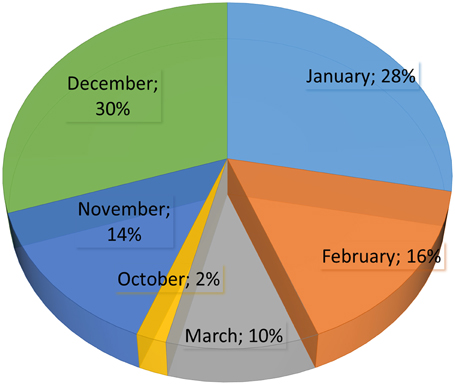
Figure 1. SACZ event percentage from November to March.

SACZ studies usually cover the time period from December to February due to the increased number of events (for example Liebmann et al., 1999). As shown in Figure 1 within the 10 years covered by this study, a higher number of events indeed occurred from December to February, but the number of SACZ events in November and March is significant, with a few occurrences in October as well. Therefore, the present study will consider the entire period from October to March to define the SACZ presence.

The study area (Figure 2) was based on the SACZ coastal influence region shown in Carvalho et al. (2002) (see their Figure 3). The choice of this region was due to its relation to summer rainfall during SACZ events and the availability of datasets with few series failures.

FIGURE 2

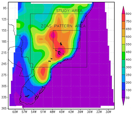
Figure 2. Total region used with its regional topography. The two squares inside in the total region represent the study area and the main position of the SACZ pattern.

FIGURE 3

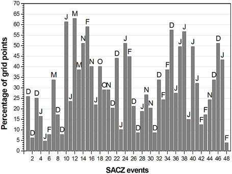
Figure 3. Percentage of grid points where SACZ events happened when considered the period from October to March.

The monthly climatology of each grid point of the study area was calculated taking into account a 30-year average. A SACZ-related precipitation extreme event was defined as the set of 7 consecutive days with at least 1 day of 35% climatology precipitation or higher, and the sum of the precipitation in the two previous and two posterior days should be equivalent to, at least, 20% of the climatology. Also, the sum of the precipitation in the three previous and three posterior days should amount to 10% of the monthly climatology, and no values should be null.

The previously selected SACZ event dates were then confronted with the dates determined by the aforementioned criterion. Events that deviated up to 2 days of the original date were considered as coincident events. The 2-day gap was included because of future climate data, which in general a month have 30 days. This calendar does not contribute to exactly locate the correct date of the SACZ event.

The above analysis is suitable for real precipitation data, as shown in Figures 3, 4. However, as numerical models do not always represent well the intra-seasonal variability, and as a consequence, systems such as SACZ (Ferraz et al., 2013), principal component analysis (PCA) was used in order to determine the mode more similar to SACZ and then the selection criterion was redefined based in the data rebuilt from the PCA series.

FIGURE 4

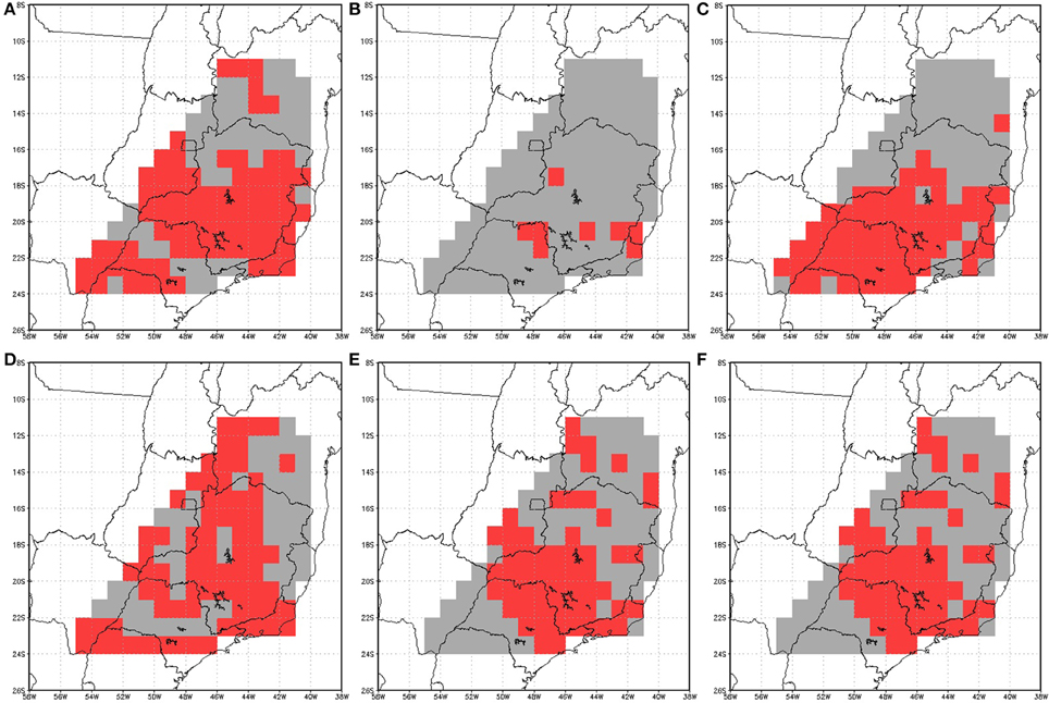
Figure 4. Spatial distribution of events with increased date coincidence between the SACZ and a criterion-selected extreme. The light gray color represents the entire study area and the dark gray color shows the coincidence area. (A) Event 10 – January, (B) Event 12 – March, (C) Event 14 – November, (D) Event 15 – February, (E) Event 22, December and (F) Event 24, January.

The new selection criterion consists of:

(1) Determining the mode maximum area and calculating an average for the period,

(2) Rebuilding the PCA series with this average,

(3) Selecting time periods when all of the following conditions are true:

(a) day(i) > 6%CLIM;

(b) ${\displaystyle {\sum }_{i=i-1}^{i+1}day(i)>10\%CLIM}$

(c) ${\displaystyle {\sum }_{i=i-2}^{i+2}day(i)>12\%CLIM}$

(d) ${\displaystyle {\sum }_{i=i-3}^{i+3}day(i)>20\%CLIM}$

The previously selected SACZ event dates were then confronted with the dates determined by the aforementioned criterion, in order to calibrate it and allow for its application to future data. This condition should be repeated for at least consecutive 3 days to be considered an event.

Results

Figure 3 shows the event percentage per grid point, that is, on how many points in the study area grid each of the 48 events is shown. The letters above each bar represent the beginning of the month when the event happened. From this Figure 1 can see that higher event frequency on a larger number of grid points (above 45%) occurred alternately in December and January, with fewer occurrences in February (2), March (1) and November (1).

As shown in Figure 4, the spatial distribution of increased coincidence grid points is set across clearly defined areas. From December to February there is an increased concentration on the states of Minas Gerais and Bahia (to the north of the Brazilian Southeastern Region), which reflects the results presented in Carvalho et al. (2002). In November, this distribution is more concentrated to the south, over São Paulo (event 14 – south of the Brazilian Southeastern Region) and in March it moves to the north, and covers part of Minas Gerais and Bahia (event 12), which suggests that the SACZ migrates from South to North throughout the summer. This variation may be related to event intensity or to the frequency period of the intra-seasonal oscillation that triggered the SACZ event. Ferraz (2004) showed differences in the oscillation periods for both areas. The southernmost area (which includes São Paulo) features more frequent oscillation (10/20 days), whereas oscillation frequency is around 30/60 days further north. A thorough analysis of these events is required for a more comprehensive explanation.

A variability method with SACZ-attributable characteristics was found through principal component analysis. Figure 5 shows the precipitation method for real data, and for present time and future climate scenarios (RCP4.5 Representative Concentration Pathways Emissions from the IPCC Fifth Assessment Report - IPCC AR5 WG1). The ZCAS position presented here agrees with that found by Lenters and Cook (1999) in their REOF 3 pattern.

FIGURE 5

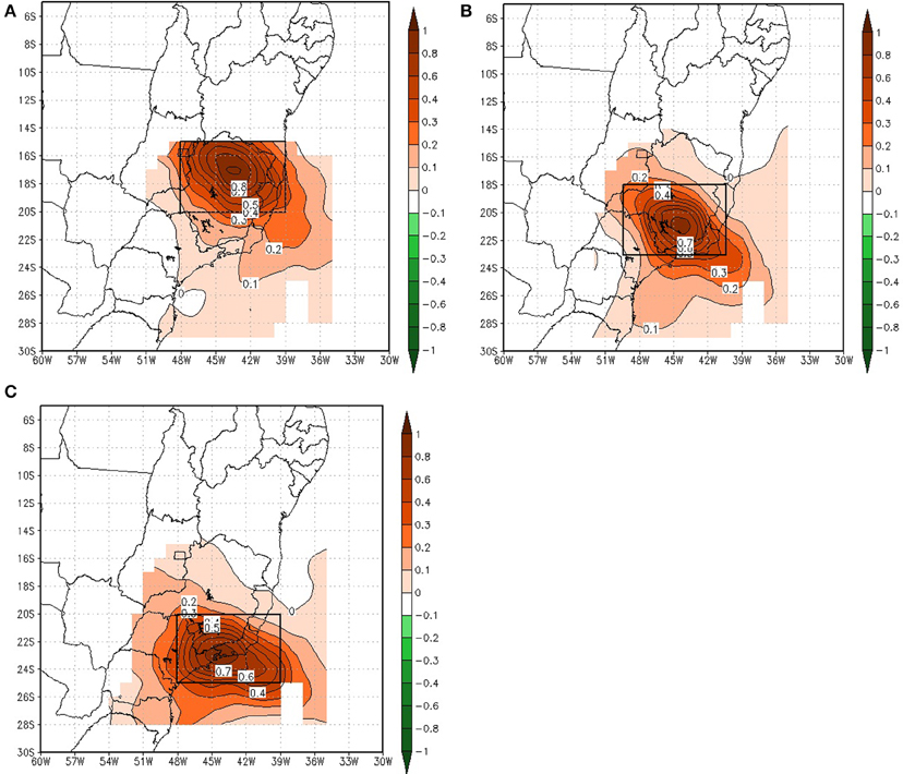
Figure 5. SACZ-related variability methods using actual precipitation data (A - top left), present (B - top right) and future time RCP4.5 (C - bottom left).

The SACZ determination criterion was applied after the maximum precipitation area (marked by a rectangle on Figure 5) had been established. Variability methods were calculated using the 17 years period in each series, but the method was only calibrated with data from the known events timeframe (1995–2005).

Sixty extreme events were selected for the LIB series, and 40 of those are coincident with an actual SACZ event. Forty-five events were selected for the PRE series where 29 of those coincide with a SACZ event. This result indicates that the criterion was accurate for 83% the SACZ cases for the LIB series, but it overestimated the number of extreme events by 25%. For the PRE series, there was 61% accuracy, but the number of events was underestimated by 9%.

Figure 6 shows the average event duration for each month, where the SACZ column represents actual events found in the literature. For present time data, it can be seen that events last 7 days on average, and they last longer from January to March and in October, and shorter in November and December. For future time data (FUT), the average number of days is bigger in January (up to 9 days), followed by December (approximately 6 days). However, assessments of individual cases reveal very long events (lasting up to 25 days) that are generally overestimated by the PRE series, but overall both the LIB and the PRE series underestimate event duration (Figure 7). Several studies have shown that HADGEM-ES data underestimate the actual precipitation (Vogel, 2012; Zhang et al., 2013; Dike et al., 2014), in particularly over the SACZ, Cavalcanti and Shimizu (2012) showed a decrease in precipitation in this region in present time. The LIB gridded fields are made by averaging all available stations within a specified radius of each grid point. The radius was chosen to be 0.75 times the grid spacing, so as to ensure that every station was included in at least one grid point. In grid points with high station density benefit from spatial smoothing by blending numerous individual observations. In regions of low station density, however, there are many gridpoint values based on a single station report or a very small number of stations (Liebmann and Allured, 2005). In this way, Liebmann and Allured (2005) explain that extreme events (heavy storms) localized in areas smaller than the grid spacing will be considerably weaked by averaging with other stations. Such aspects may explain the decrease in intensity of events presented in Figure 6, in relation to real events.

FIGURE 6

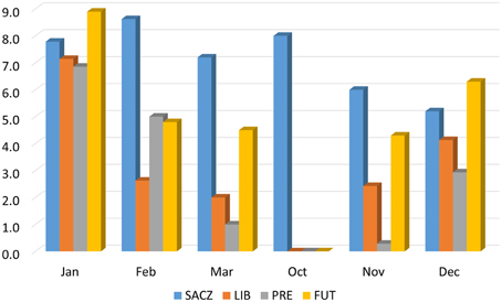
Figure 6. Average duration of actual SACZ events (blue bar) detected by the criterion in the LIB (orange) and PRE series (gray), and events detected in the FUT series (yellow).

FIGURE 7

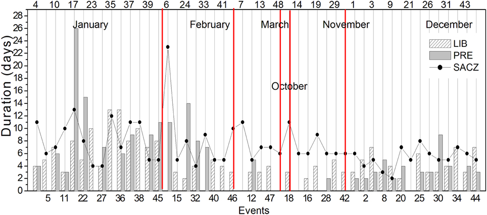
Figure 7. Duration (in days) of each SACZ event: actual (line), and detected by the criterion for the LIB (hatched bar) and PRE (gray bar) series.

When average precipitation in the maximum precipitation areas is compared for the 48 events (regardless how they were detected), it is clear that PRE data overestimates precipitation in the area (LIB), which may explain the increased number of events detected by the criterion in this data series (Figure 8). As for future climate scenario data (FUT), the increase is even more significant in every month. Cavalcanti and Shimizu (2012) showed an increase in precipitation in the SACZ region in the future data during Austral summer.

FIGURE 8

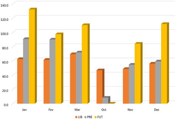
Figure 8. Average precipitation in the method area, weighed by the number of events, during the 48 SACZ episodes for the LIB (orange) and PRE (green) series, and during the 73 episodes detected in the FUT series (violet).

When applied to the 17 years of data available for the FUT series, the criterion revealed 73 events distributed according to Figure 9. Event distribution was similar to the present climate, with more events from December to February, whereas for the other months the number of events was slightly lower for the future climate. Looking at the event duration one can see a few long events in January and December; they are, however, shorter than the ones found in present climate (Figure 10).

FIGURE 9

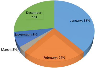
Figure 9. SACZ event percentage from November to March for future time.

FIGURE 10

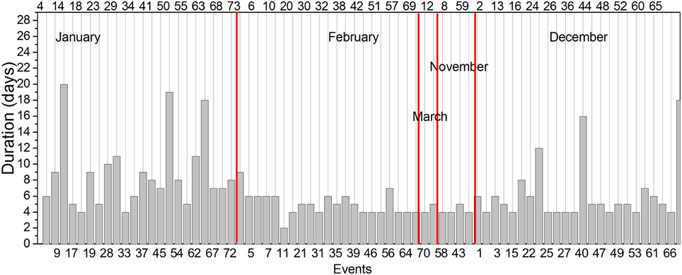
Figure 10. Duration (in days) of every SACZ event simulated for the FUT series.

Discussion

The SACZ event detection criterion proposed here showed quite satisfactory results when event dates were compared with previously known ones. When it was applied to future climate it identified a number of events compatible with the studied timeframe. The SACZ was well defined for both the simulated and observed precipitation data.

Considering the 60 months of data reviewed, 48 SACZ events were found (0.8 event/month); for future climate, there were 96 months of data and 73 events were found (0.76 events/month). This might suggest a slight reduction in the number of future events, however, there are a few points to consider: when this number is compared with the model simulation, 45 events were found, where 65% coincides with events that happened and 35% are coincident with method-detected events that did not happen. This means that, from the 73 events, only 49 would actually happen, which could suggest a significant reduction in the number of the events in the future when compared to the present time. On the other hand, even with the chance of a reduction in the number of events, this would not be directly related to precipitation numbers, as the accumulated average for event months reveals an increase of 55% in precipitation for future climate, which suggests fewer, but more intense events.

Despite being able to determine the characteristics of most of the SACZ events analyzed, the index presented in this study overestimated the number of events. It should be emphasized that we are proposing an objective criterion based only on precipitation, because this variable is easily obtained from general circulation models that simulates past, present and future climate, contrary to OLR and some other variables used nowadays. Of course, this is a first step to identify the SACZ through a simple objective analysis. Further work is still necessary to improve this method and it will be presented elsewhere.

Conflict of Interest Statement

The authors declare that the research was conducted in the absence of any commercial or financial relationships that could be construed as a potential conflict of interest.

Acknowledgments

The authors would like to acknowledge FAPESP (n° 08/58101-9) and CNPq for the financial support.

References

Ambrizzi, T., and Hoskins, B. J. (1997). Stationary Rossby wave propagation in a baroclinic atmosphere. Q. J. Roy. Meteorol. Soc. 123, 919–928. doi: 10.1002/qj.49712354007

CrossRef Full Text | Google Scholar

Ambrizzi, T., Silva Dias, P. L., and Grimm, A. M. (1994). “A comparison between barotropic and baroclinic remote responses associated with the SPCZ and SACZ,” in II Congresso Latino-Americano e Ibérico de Meteorologia e VIII Congresso Brasileiro de Meteorologia, 1994, Belo Horizonte, MG. Anais do II Congresso Latino-Americano e Ibérico de Meteorologia e VIII Congresso Brasileiro de Meteorologia, Vol. 2 (Belo Horizonte: Sociedade Brasileira de Meteorologia), 85–87.

Barreiro, M., Chang, P., and Saravanan, R. (2002). Variability of the South Atlantic Convergence Zone simulated by an atmospheric general circulation model. J. Clim. 15, 745–763. doi: 10.1029/2003GL018647

CrossRef Full Text | Google Scholar

Carvalho, L. M. V., Jones, C., and Liebmann, B. (2002). Extreme precipitation events in Southeastern South America and large-scale convective patterns in the South Atlantic Convergence Zone. J. Clim. 15, 2377–2394. doi: 10.1175/1520-0442(2002)015<2377:EPEISS>2.0.CO;2

CrossRef Full Text | Google Scholar

Carvalho, L. M. V., Jones, C., and Liebmann, B. (2004). The South Atlantic Convergence Zone: persistence, intensity, form, extreme precipitation and relationships with intraseasonal activity. Clim. J. 17, 88–108. doi: 10.1175/1520-0442(2004)017<0088:TSACZI>2.0.CO;2

CrossRef Full Text

Casarin, D. P., and Kousky, V. E. (1986). Anomalias de precipitacão no sul do Brasil e variaçõs na circulaçoes atmosférica. Rev. Bras. Meteorol. 1, 83–90. doi: 10.1175/1520-0442(2004)017<0088:TSACZI>2.0.CO;2

CrossRef Full Text | Google Scholar

Cavalcanti, I. F. A., and Shimizu, M. H. (2012). Climate fields over South America and variability of SACZ and PSA in HadGEM2-ES. Am. J. Clim. Change 1, 132–144. doi: 10.4236/ajcc.2012.13011

CrossRef Full Text | Google Scholar

Dike, V. N., Shimizu, M. H., Diallo, M., Lin, Z., Nwofor, O. K., and Chineke, T. C. (2014). Modelling present and future African climate using CMIP5 scenarios in HadGEM2−ES. Int. J. Climatol. doi: 10.1002/joc.4084. [Epub ahead of print].

CrossRef Full Text | Google Scholar

Farrara, J. D., Ghil, M., Mechoso, C. R., and Mo, K. C. (1989). Empirical orthogonal functions and multiple flow regimes in the Southern Hemisphere winter. J. Atmos. Sci. 46, 3219–3223.

Google Scholar

Ferraz, S. E. T. (2004). Oscilações Intrasazonais no Sul e Sudeste do Brasil Durante o Verão. Tese (Doutorado) - Instituto de Astronomia, Geofísica e Ciências Atmosféricas da Universidade de São Paulo, São Paulo.

Ferraz, S. E. T., Souto, R. P., Dias, P. L. S., Velho, H. F. C., and Ruivo, H. M. (2013). Analysis for precipitation climate prediction on south of Brazil. Ciência e Natura 496–500. doi: 10.5902/2179-460X12253

PubMed Abstract | Full Text | CrossRef Full Text | Google Scholar

Ferreira, N. J., Sanches, M., and Silva Dias, M. A. F. (2004). Composição da zona de convergência do atlântico sul em Períodos de el Niño e la Niña. Rev. Bras. Meteorol. 19, 89–98.

Figueroa, S. N., Satyamurty, P., and Silva Dias, P. L. (1995). Simulation of the summer circulation over the South American region with an Eta coordinate model. J. Atmos. Sci. 52, 1573–1584.

Google Scholar

Giorgi, F., Marinucci, M. R., and Bates, G. T. (1993). Development of a second generation regional climate model (RegCM2). Part I: Boundary layer and radiative transfer processes. Mon. Wea. Rev. 121, 2794–2813.

Google Scholar

Grimm, A. M., and Silva Dias, P. L. (1995). Analysis of tropical—extratropical interactions with influence functions of a barotropic model. J. Atmos. Sci. 52, 3538–3555.

Google Scholar

Kidson, J. W. (1988). Interannual variations in the Southern Hemisphere circulation. J. Clim. 1, 1177–1198.

PubMed Abstract | Full Text Google Scholar

Kiladis, G. N., and Weickmann, K. M. (1992). Circulation anomalies associated with tropical convection during northern winter. Mon. Wea. Rev. 120, 1900–1923.

Google Scholar

Kiladis, G., and Weickmann, K. M. (1997). Horizontal structure and seasonality of large scale circulations associated with submonthly tropical convection. Mon. Wea. Rev. 125, 1997–2013.

Google Scholar

Kodama, Y.-M. (1992). Large-scale common features of subtropical precipitation zones (the Baiu frontal zone, the SPCZ, and the SACZ), Part I: characteristics of subtropical frontal zones. J. Meteorol. Soc. Jpn. 70, 813–835.

Google Scholar

Kodama, Y.-M. (1993). Large-scale common features of sub-tropical convergence zones (the Baiu frontal zone, the SPCZ, and the SACZ), Part II: conditions of the circulations for generating the STCZs. J. Meteorol. Soc. Jpn. 71, 581–610.

Google Scholar

Krishinamurti, T. N., Kanamitsu, M., Koss, W. J., and Lee, J. D. (1973). Tropical east-west circulation during the Northern winter. J. Atmos. Sci. 30, 780–787.

Google Scholar

Lenters, J. D., and Cook, K. H. (1995). Simulation and diagnosis of the regional South American precipitation climatology. Clim. J. 8, 2988–3005.

Google Scholar

Lenters, J. D., and Cook, K. H. (1999). Summertime precipitation variability over South America: role of the large-scale circulation. Mon. Wea. Rev. 127, 409–431.

Google Scholar

Liebmann, B., and Allured, D. (2005). Daily precipitation grids for South America. Bull. Am. Meteorol. Soc. 86, 1567–1570. doi: 10.1175/BAMS-86-11-1567

CrossRef Full Text | Google Scholar

Liebmann, B., Jones, C., and Carvalho, L. M. V. (2001). Interannual variability of daily extreme precipitation events in the State of São Paulo. J. Clim. 14, 208–218. doi: 10.1175/1520-0442(2001)014<0208:IVODEP>2.0.CO;2

CrossRef Full Text | Google Scholar

Liebmann, B., Kiladis, G. N., Marengo, J. A., Ambrizzi, T., and Glick, J. D. (1999). Submonthly convective variability over South America and the South Atlantic Convergence Zone. J. Clim. 12, 1877–1891. doi: 10.1175/1520-0442(1999)012<1877:SCVOSA>2.0.CO;2

CrossRef Full Text | Google Scholar

Madden, R. A., and Julian, P. R. (1994). Observations of the 40-50 day oscillation —A review. Mon. Wea. Rev. 122, 814–837.

Google Scholar

Mo, K. C., and Ghil, M. (1987). Statistics and dynamics of persistent anomalies. J. Clim. 44, 877–902.

PubMed Abstract | Full Text | Google Scholar

Paegle, J. N., Byerle, L. A., and Mo, K. C. (2000). Intraseasonal modulation of South American summer precipitation. Mon. Wea. Rev. 128, 837–850. doi: 10.1175/1520-0493(2000)128<0837:IMOSAS>2.0.CO;2

CrossRef Full Text | Google Scholar

Paegle, J. N., and Mo, K. C. (1997). Alternating Wet and Dry Conditions over South America during Summer. Mon. Wea. Rev. 125, 279–291.

Google Scholar

Quadro, M. F. L. (1994). South Atlantic Convergence (SACZ) Studies Over South America. Master of Meteorology—National Space Agency Institute, São José dos Campos (available in Portuguese).

Robertson, A. W., and Mechoso, C. R. (2000). Interannual and interdecadal variability of the South Atlantic Convergence Zone. Mon. Wea. Rev. 128, 2947–2957. doi: 10.1175/1520-0493(2000)128<2947:IAIVOT>2.0.CO;2

CrossRef Full Text | Google Scholar

Sanches, M. B., and Silva Dias, M. A. F. (1996). Summer Synoptic Analysis—South Atlantic Convergence Zone influence (SACZ). In: 9° Brazilian Congress of Meteorology, Campos do Jordão. Ann. Braz. Meteorol. Soc. 1, 439–443. [Available in Portuguese].

Siqueira, J. R., and Machado, L. A. T. (2004). Influence of the frontral systems on the day-to-day convection variability over South America. J. Clim. 17, 1758–1766. doi: 10.1175/1520-0442(2004)017<1754:IOTFSO>2.0.CO;2

CrossRef Full Text | Google Scholar

Siqueira, J. R., Rossow, W. B., Machando, L. A. T., and Pearl, C. (2005). Structural characteristics of convective systems over South America related to cold-frontal incursions. Mon. Wea. Rev. 133, 1045–1064. doi: 10.1175/MWR2888.1

CrossRef Full Text | Google Scholar

Streten, N. A. (1973). Some characteristics of the satellite-observed bands of persistent cloudiness over the Southern Hemisphere. Mon. Wea. Rev. 101, 486–495.

Google Scholar

Taljaard, J. J. (1972). The clouds bands of the South Pacific and Atlantic Oceans. Meteorol. Monogr. 13, 189–192.

Vogel, D. (2012). Changes in Precipitation Characteristics and Extremes - Comparing Mediterranean to North-Western European Precipitation. Master degree Thesis, Institute of Atmospheric and Climate Science, University of Reading.

Yassunary, T. (1977). Stationary waves in the Southern Hemisphere mid-latitude zonal revealed from average brightness charts. J. Meteorol. Soc. Jpn. 55, 274–285.

Google Scholar

Zhang, H., Fraedrich, K., Blender, R., and Zhu, X. (2013). Precipitation extremes in CMIP5 simulations on different time scales. J. Hydrometeorol. 14, 923–928. doi: 10.1175/JHM-D-12-0181.1

CrossRef Full Text | Google Scholar