Bayesian inference for stochastic individual-based models of ecological systems: a pest control simulation study

1. Introduction

The use of mathematical models in population ecology and epidemiology has a long history (Murray, 2002). Among the wide range of available models, two major categories can be distinguished: population-level and individual-based models (Black and McKane, 2012). Population-level models (PLMs) implicitly assume an infinite population size and provide a phenomenological description of the overall population behavior. The main advantage of PLMs is that they involve ordinary differential equations that can be analyzed using dynamical systems theory; their main drawback is that they neglect any effect that may be caused by finite population sizes or by the inherently random nature of interactions between individuals. Individual-based models (IBMs), on the other hand, are discrete models that represent an ecological system as a collection of a finite number of individuals that are modeled explicitly (DeAngelis and Mooij, 2005; Railsback and Grimm, 2012). Depending on how many details are included for each individual, IBMs can be further distinguished into agent-based models, which provide great detail but are limited to algorithmic and numerical analysis, and stochastic process models that typically distinguish a limited number of different types of individuals but are more amenable to analytical investigation (Black and McKane, 2012). Among IBMs we restrict our attention to stochastic process models where the possible interactions of species occur with a probability that is proportional to the number of individuals present in the system. Mathematically, these models can be represented by continuous-time discrete-state Markov chains (CTMCs).

Discrete stochastic models naturally arise in many applications both in ecology (Marion et al., 1998; Ovaskainen and Cornell, 2006; Ovaskainen and Meerson, 2010) and in epidemiology (Isham, 1991; Nåsell, 2002). While stochastic IBMs and CTMCs in particular, provide an intuitive description of these systems, their analysis tends to be difficult. Consequently, the use of these models has for a long time remained limited to systems containing at most a handful of different interacting species. Recent years have seen, on the one hand, an immense increase in computational resources, and on the other hand, a surge of studies in which IBMs have been used to study biological systems at the cellular level. Specifically, in these applications interacting molecules play the role of interacting individuals (Balazsi et al., 2011; Goutsias and Jenkinson, 2013; Neuert et al., 2013). These developments have stimulated research on new methods for analyzing IBMs (see, e.g., Munsky and Khammash, 2006; Wolf et al., 2010; Ruess et al., 2011, 2013), which opened the path for using larger and more complicated models that are more suitable to represent the complex systems encountered in applications. As a consequence of these new modeling capabilities, problems that were for a long time solvable only using PLMs can now be analyzed (and hence receive renewed interest) in the context of IBMs. In the case study of this paper, for example, we consider the use of IBMs to address optimal control problems for pest management. Many studies on optimal control problems in ecology were performed using PLMs during the 1970's (see Wickwire, 1977 and references therein). In these pioneering works, the control actions were usually included by changing the model parameters (e.g., birth or death rates) according to the control action or by developing a new model for the controlled system, in which the control is included as a continuous input. In the case study presented here, we adopt a different modeling approach, similar to the idea presented in Jaquette (1970) for a simple birth-death process. Specifically, we assume that the control operator can reset the state of the system (for example reduce the number of pest individuals by applying pesticide) at certain given intervention times, while the dynamics of the system between the reset times follow the uncontrolled IBM. The resulting model is thus a stochastic hybrid system with controlled state reset (Branicky et al., 1998; Bensoussan and Menaldi, 2000).

In the 1970's, the main difficulty in translating the control theoretical studies into real world applications was the lack of efficient and accurate procedures to estimate the required model parameters (Wickwire, 1977). While for PLMs these difficulties have been to a large extent overcome, for the more detailed IBMs the problem of reverse engineering parameter values from measured data is still a major challenge (Poovathingal and Gunawan, 2010; Stumpf, 2014). Most of the available approaches, in fact, require iterative evaluation of parameter likelihoods, which are usually not available analytically and computationally very expensive. To circumvent this problem, likelihood-free approaches for parameter inference, such as approximate Bayesian computation, have found applications in ecology (McKinley et al., 2009; Lagarrigues et al., 2014) and other fields (Toni et al., 2009).

In this paper, we suggest a different approach for parameter inference based on an expression that allows for fast (but approximate) evaluation of the likelihood. To obtain this expression, we move from a full description of the stochastic model to ordinary differential equations that describe the time evolution of only means and (co)variances (and possibly higher order moments) of the interacting species. We then use moment closure techniques to approximate the solution of these equations and show that the results can be used to approximate the likelihood. Moment closure methods have a long history in population biology (Whittle, 1957; Nåsell, 2003; Krishnarajah et al., 2005; Singh and Hespanha, 2006; Hespanha, 2008), but only recently first attempts have been made to use these methods for parameter inference (Kügler, 2012; Zechner et al., 2012; Milner et al., 2013). The approach we take here is motivated by recent developments in the modeling of biochemical reaction networks (Zechner et al., 2012) and differs from typical methods in ecology (Ross et al., 2009; Gillespie and Golightly, 2010) in that it is intended to be used with data that are obtained from many independent observations of a system, instead of being tailored to a single observation of an ecological system over time. Accordingly, it is most suitable for applications in which many replicates of the same experiment can be performed, as typically done in microcosm and mesocosm experiments (Srivastava et al., 2004; Hekstra and Leibler, 2012; Altermatt et al., 2014), but only one measurement per replica is feasible. This might be the case when measurements are costly or time-consuming, resulting in a trade-off between the number of measurements and the number of replicates (e.g., Carrara et al., 2014), or if they perturb the system so that further measurements of the same replicate are not possible or meaningful. This is the typical scenario for destructive measurements as, for instance, in the study of bacterial colonization dynamics where measurements may require sequencing the bacterial genomes of the whole community (Cordero et al., 2012). At the subcellular scale, this type of data is naturally obtained when the experimental replicates are individual cells and the intracellular dynamics of chemical species are measured (e.g., Zechner et al., 2012).

2. Materials and Methods

2.1. Individual-Based Modeling

Consider an ecological system comprising m species, X₁, …, X_m that can interact, in a given habitat, according to K different types of interactions

$\begin{array}{cc}{\nu }_{1k}^{\prime }{X}_1+\dots +{\nu }_{mk}^{\prime }{X}_m\stackrel{{\theta }_k}{\to }{\nu }_{1k}^{″}{X}_1+\dots +{\nu }_{mk}^{″}{X}_m,k=1,\dots ,K.& (1)\end{array}$

The expression on the left hand side of the arrow denotes the amount ν′_ik of individuals for each species X_i needed for interaction k to happen. The expression on the right hand side describes the result of the interaction. In other words, the effect of interaction k is to update the number of individuals of each species X_i by the net amount ν_ik: = ν″_ik − ν′_ik. Let $X(t)={\left[X_1(t)\cdots X_m(t)\right]}^{\top }$ denote the amount of individuals of each species present in the system at time t. In the following, we assume that each interaction is a stochastic event whose probability to occur depends on the probability that the required amounts of individuals meet in some location of the habitat and on a parameter θ_k that determines the probability that the individuals successfully interact when they meet. Since the interactions are stochastic events, X(t) is a stochastic process that takes values x = [x₁ … x_m]^⊤ ∈ ℕ^m₀. Under the assumption of random movement of the individuals, the probability that a given interaction takes place in the infinitesimal time interval [t, t + dt], given the current population state X(t) = x, can be determined by the law of mass action as

$\begin{array}{l}{a}_k(x,\theta )dt:={\theta }_k{h}_k(x)dt,\text{where}{h}_k(x)={\displaystyle \prod _{i=1}^m\left(\begin{array}{c}{x}_i\\ {\nu }_{1k}^{\prime }\end{array}\right)},\\ k=1,\dots ,K\text{and}\theta =\left\{{\theta }_1,\dots ,{\theta }_K\right\}.\end{array}$

Note that we assumed that the habitat is homogeneous, that is, the probabilities a_k(x, θ)dt do not depend on the spatial location, but only on the total amount x of individuals present in the system.

2.2. Data Description

Since the model introduced in the previous section is stochastic, for a given initial population X(0) = x₀, many different evolutions of the system, corresponding to different realizations of the stochastic process X(t), are possible. In the following, we assume that we can monitor many of these different replicates of the system, but only one measurement per replica can be taken (possibly at different times). Therefore, the collected data consists of several measurements of the number of individuals of one species¹ X_j at different time points, each coming from a different replicate. This means that we assume that the collected data contains information about the dynamics but not about the correlation of the species abundance between different time points. Let t₁, …, t_S denote the measurement times and suppose that for each measurement time we have measured n different replicates². The data set is then of the form $D={\left\{X_j^1(t_s),\dots ,X_j^n(t_s)\right\}}_{s=1}^S$, where all the measurements Xⁱ_j(t_s), i = 1, …, n, s = 1, …, S are statistically independent.

A feature of such data, which is at the same time a strength and a serious complication, is that the measurements described above correspond to observations from n · S (supposedly) identical replicates of the system. In a realistic situation, these replicates might be performed in different days or come from slightly different ambient conditions. Not taking into account this source of variability can have deleterious effects on model predictions and accordingly also on any strategy for optimal interventions and population control. Consequently, the variability observed in different replicates is an asset that should be used in order to identify a model that is not tailored to one particular experimental condition but can describe all of them. To allow this type of flexibility, we assume that in different repetitions of an experiment some of the parameters θ_k, k = 1, …, K may be slightly different. Without loss of generality, let us denote by k = 1, …, r the interactions for which the rate θ_k varies between different repetitions of the experiment, and by k = r + 1, …, K the remaining ones that are the same for all repetitions. We describe the experimental variability by assuming that the success of the first r interactions is given by θ_k · Z_k, k = 1, …, r, where Z = [Z₁ … Z_r]^⊤ is a random vector with unknown distribution P_Z. Moreover, we assume that the marginal means of P_Z are all equal to one, so that θ_k, k = 1, …, r are the average interaction success rates over different replicates of the experiment. This gives rise to a model akin to mixed-effects models in the statistics literature (Lavielle, 2014).

2.3. The Conditional Master Equation and Moment Dynamics

Under the assumption of a homogeneous environment, for fixed success parameters θ_k, the time evolution of the number of individuals X(t), as described in Section 2.1, follows a continuous-time Markov chain. Consequently, the time evolution of its probability distribution p(x, t): = P[X(t) = x], can be described by a master equation (Black and McKane, 2012). The same theory holds in the case of random success rates θ_k · Z_k, k = 1 …, r, if we fix a specific realization z of the random vector Z. Mathematically, the conditional process X(t) | Z = z is Markovian and can be described by the master equation

$\begin{array}{cc}\begin{array}{l}\dot{p}(x,t|z)=-p(x,t|z){\displaystyle \sum _{k=1}^K{a}_k(x,\theta ,z)}\\ +{\displaystyle \sum _{k=1}^{K}p(x-{\nu }_k,t|z)a_k(x-{\nu }_k,\theta ,z)},\end{array}& (2)\end{array}$

where³ p(x, t|z) : = P[X(t) = x|Z = z]. Typically, Equation (2) cannot be solved explicitly and for complex systems also numerical approaches might fail. However, if one is not interested in the whole probability distribution, Equation (2) can be used to derive evolution equations for some of the moments of the distribution, as mean and variance. Specifically, denoting by $\tilde{\psi }$ the l-dimensional vector of the (uncentered) moments up to some order L of the joint process $\tilde{X}$(t) = [X(t)^⊤ Z^⊤]^⊤ and by $\overline{\tilde{\psi }}$ the vector containing the higher order moments of $\tilde{X}$(t), one obtains

$\begin{array}{cc}\frac{d}{dt}\tilde{\psi }(t)=\tilde{A}(\theta )\tilde{\psi }(t)+\tilde{B}(\theta )\overline{\tilde{\psi }}(t),& (3)\end{array}$

where $\tilde{A}$(θ) ∈ ℝ^{l × l} and $\tilde{B}$(θ) ∈ ℝ^{l × ∞} are matrices defined by the reaction network and by the parameters θ [a detailed derivation is given in Zechner et al. (2012)]. For mass action kinetics with at most pairwise interactions of the species, $\overline{\tilde{\psi }}$ contains moments of order at most L + 2, so that $\tilde{B}$(θ) is a finite dimensional matrix (Ruess and Lygeros, 2015). Nonetheless, the system in Equation (3) is not solvable because it depends on the unknown quantities $\overline{\tilde{\psi }}$(t) (which act as an external input, that is, they are not part of the state vector). To overcome this issue, one can use moment closure techniques to approximate the unknown higher order moments $\overline{\tilde{\psi }}$(t) by non-linear functions of the lower order moments, that is, $\overline{\tilde{\psi }}(t)\cong \tilde{f}(\tilde{\psi }(t))$. As a consequence, the right hand side of Equation (3) can be approximated with an expression that depends only on the state variables leading to the solvable closed system

$\begin{array}{cc}\frac{d}{dt}\tilde{\nu }(t)=\tilde{A}(\theta )\tilde{\nu }(t)+\tilde{B}(\theta )\tilde{f}(\tilde{\nu }(t)).& (4)\end{array}$

Note that in Equation (4) we used a different symbol for the state vector to stress the fact that $\tilde{\nu }$(t) are approximations of the true moments $\tilde{\psi }$(t), since they are obtained as solution of the approximated dynamics.

Given that the marginal moments corresponding to Z of the joint process $\tilde{X}$(t) are constant, we can write Equation (4) as

$\begin{array}{cc}\frac{d}{dt}\nu (t)=A(\theta )\nu (t)+C(\theta ){\mu }^Z+B(\theta )f(\nu (t),{\mu }^Z),& (5)\end{array}$

where ν(t) are the moments of $\tilde{X}$(t) excluding the marginal moments of Z, μ^Z are the moments of Z up to order L and the matrices A(θ), B(θ), C(θ) are sub-matrices of $\tilde{A}$(θ), $\tilde{B}$(θ). This form of the equations is convenient because we can now regard the moments μ^Z as additional parameters and the system of moment equations for ν(t) as being parameterized by $\gamma =\left\{\theta ,{\mu }^Z\right\}$. Consequently, for a specified parameter vector γ, the system of Equation (5) can be solved numerically allowing one to compute any desired moment of X(t) up to order L.

2.4. Bayesian Inference with Population Data

In real applications, usually neither the rates θ nor the variability μ^Z between repetitions of the experiments are known. Hence, to obtain a model that is useful in practice, we need to estimate the parameters γ from measured data. This task can be posed as a Bayesian parameter inference problem, where any available knowledge about γ can be specified as an a priori parameter distribution p(γ). The result of the Bayesian inference procedure is a parameter posterior distribution p(γ | d) that reflects the updated belief about γ, given the observed realization d of the data D. According to Bayes' rule, this posterior distribution can be obtained as

$p(\gamma |d)=\frac{p(d|\gamma )·p(\gamma )}{p(d)},$

where p(d | γ) is the likelihood of γ for the observed realization d, p(γ) is the prior distribution, and p(d) = ∫ p(d|γ) p(γ) dγ is the marginal likelihood of the data. Since computing the posterior distribution analytically is usually impossible, Monte Carlo schemes are typically used to draw samples γ₁, …, γ_M, from p(γ | d), allowing one to construct an empirical estimate of the posterior distribution. The iterative evaluation of the likelihood p(d | γ), needed in these schemes, can however be computationally very expensive or even impossible for complex high dimensional systems. For the data considered in this paper, for example, evaluating the parameter likelihood requires computing the distribution of the measured species at all the measurement time points. Specifically, the likelihood is given by

$p(d|\gamma )={\displaystyle \prod _{s=1}^S{\displaystyle \prod _{i=1}^{n}P\left[X_j^i(t_s)=x_j^i(t_s)|\gamma \right]}}={\displaystyle \prod _{s=1}^S{\displaystyle \prod _{i=1}^n{p}_j(x_j^i(t_s),t_s|\gamma )}},$

where p_j(·, t|γ) is the distribution of species X_j at time t given that γ are the model parameters, and xⁱ_j(t_s), i = 1, …, n, s = 1, …, S are the measured abundances of species X_j. The factorization of the joint distribution over time points and samples stems from the assumption that all the measurements are statistically independent. It is evident that evaluating this likelihood requires computing p_j(·, t|γ). This cannot be done (except in some special cases) without first computing the entire joint distribution of $\tilde{X}$(t) at all the measurement time points, hence solving Equation (2). For these reasons, exact Bayesian inference is very difficult, if not impossible.

A naive idea to overcome these issues would be to approximate p_j(·, t|γ) by using the moments computed according to Equation (5) together with the assumption that p_j(·, t|γ) belongs to a certain family (e.g., that it is a Gaussian distribution). Such assumptions are, however, in general not satisfied and, as detailed in the following, they are not really necessary. By using as data the first L moments of the measured samples only, it is in fact possible to derive a different likelihood function that is correct for any distribution p_j(·, t|γ), in the limit of n → ∞. Specifically, set L = 2 and let $\widehat{\mu }$₁(t_s) and $\widehat{\mu }$₂(t_s) be sample mean and variance of the random samples $D(t_s)=\left\{X_j^1(t_s),\dots ,X_j^n(t_s)\right\}$, which represent the measured species abundances at time t_s, s = 1, …, S. Furthermore, denote by μ₁(t) the mean and by μ_i(t), i = 2, … 4, the centered moments up to order four of p_j(·, t|γ). By the central limit theorem, the probability density function p_{$\widehat{\mu }$}(· | γ) of $\widehat{\mu }:={\left[\widehat{\mu }{(t_1)}^{\top }\cdots \widehat{\mu }{(t_S)}^{\top }\right]}^{\top }$, where $\widehat{\mu }(t_s):={\left[{\widehat{\mu }}_1(t_s){\widehat{\mu }}_2(t_s)\right]}^{\top }$ is the vector of sample moments up to order 2 at time t_s, is for n large enough given by

Equation (6) allows one to evaluate the likelihood for the collection of sample moments $\widehat{\mu }$ up to order two, given the first four moments of p_j(·, t|γ). These moments can be obtained efficiently by numerically solving Equation (5). Consequently, using this approach it becomes feasible to draw samples from p(γ | $\widehat{\mu }$) using a Markov chain Monte Carlo scheme. The downside is that, by transitioning from the full data to the sample moments up to order L = 2, all the information about the parameters γ that might have been provided by higher order statistics of the data is discarded (Ruess and Lygeros, 2013). However, formulas for the likelihood of sample moments up to any desired order L can be obtained in exactly the same way, and thus, this approach is not limited to sample means and variances only. Evaluating the likelihood for sample moments up to order L requires computing moments of p_j(·, t|γ) up to order 2L, which becomes computationally expensive for large L. The choice of how many sample moments to include in the parameter inference is therefore a trade-off between computational cost and neglected information.

3. Case Study: Optimal Pest Control

3.1. The Model

As case study we consider the problem of modeling, and eventually controlling, the evolution of an agricultural pest. To this end, we consider an extension of the model of cotton aphids proposed in Matis et al. (2007) and Gillespie and Golightly (2010). Specifically, we introduce an additional immigration term to the original model and we include a recovery process of the habitat. In more detail, our model consists of a discrete state stochastic process N(t) that describes the size of the current pest population and a discrete state stochastic process C(t) that is used as an indicator of how much the environment has been deteriorated, up to time t, by the infestation. In the following, we assume that these two processes are updated according to the occurrence of the following stochastic events:

$\begin{array}{cc}\begin{array}{ccc}\varnothing & \stackrel{\alpha }{\to }& N+C\\ N& \stackrel{\lambda Z}{\to }& 2N+C\\ N+C& \stackrel{\eta }{\to }& C\\ C& \stackrel{r}{\to }& \varnothing .\end{array}& (7)\end{array}$

Specifically, we suppose that new pest individuals arise in the system due to immigration, with rate α, or birth events, with a rate that is proportional to the current population size. To capture variability between different replicates, stemming for instance from different ambient conditions, we assume that the birth rate is given by λN(t)Z, where Z is a one-dimensional random variable distributed according to a log-normal distribution P_Z with mean one and unknown variance. The death rate of the pest is given by ηN(t)C(t), i.e., it depends on the current population size, but also on the damage to the environment.

Furthermore, we assume that the process describing the state of the environment, C(t), is increased by one unit whenever a new pest individual is added in the system (either via immigration or due to a birth event). Since pest individuals deteriorate the environment for a time period that may exceed their own life span, we assume that the death of pest individuals leaves C(t) unchanged. However, we model the fact that the environment may eventually recover by assuming that C(t) decreases with rate rC(t).

This model induces a conditional master equation, see Equation (2), with state x = [n c]^⊤ and parameters θ = {α, λ, η, r}, in which a_k(x, θ, z) and ν_k, k = 1, …, 4 are given by

$\begin{array}{l}{a}_1(x,\theta ,z)=\alpha ,{\nu }_1=\left[\begin{array}{c}1\\ 1\end{array}\right],\\ a_2(x,\theta ,z)=\lambda ·n·z,{\nu }_2=\left[\begin{array}{c}1\\ 1\end{array}\right],\\ a_3(x,\theta ,z)=\eta ·n·c,{\nu }_3=\left[\begin{array}{c}-1\\ 0\end{array}\right],\\ a_4(x,\theta ,z)=r·c,{\nu }_4=\left[\begin{array}{c}0\\ -1\end{array}\right].\end{array}$

From this master equation we can derive moment equations and use moment closure to obtain a closed system in the form of Equation (5). In the following, we use equations for the moments up to order four and a fifth-order derivative matching closure, as described in Singh and Hespanha (2006). Solving the resulting approximate systems, for given parameter values θ and given first two moments of Z, enables us to approximately compute the moments of X(t) = [N(t)C(t)]^⊤ up to order four.

3.2. Inference Results

Since we assumed that Z has a log-normal distribution with mean one, it is sufficient to include only the variance of Z as an unknown parameter, so that γ = {θ, Var[Z]}. For the in silico case study, we assume that N(0) = C(0) = 0, that is initially no pests are present in the system, and that the true values of the parameters are given by

$\begin{array}{cc}\begin{array}{l}\alpha =0.03,\lambda =0.012,\eta =0.25·{10}^{-4},\\ r=0.003\text{and}\text{Var}\left[Z\right]=0.05,\end{array}& (8)\end{array}$

where we used hours as time units. These parameters produce pest outbreaks that are on the timescale of realistic profiles of aphids pest infestations. As hypothetical data set $D={\left\{N^1(t_s),\dots ,N^n(t_s)\right\}}_{s=1}^S$, we consider a case study in which n = 100 different replicates of the system are measured once a week (t_s = 7 · 24 · s hours) for a total of S = 5 weeks. We note that the chosen measurements times are consistent with the dynamics generated by the parameters given in Equation (8). If, as in real scenarios, the parameters and hence the timescale of the systems dynamics are not known one may use a sequential experiment design approach to produce informative datasets. To generate the dataset considered in this in silico case study we used the stochastic simulation algorithm (SSA), described in Gillespie (1976), with randomly drawn values z from P_Z. The sample means and variances of the data are denoted by $\widehat{\mu }={\left[\widehat{\mu }{(t_1)}^{\top }\cdots \widehat{\mu }{(t_5)}^{\top }\right]}^{\top }$ where $\widehat{\mu }(t_s):={\left[{\widehat{\mu }}_1(t_s){\widehat{\mu }}_2(t_s)\right]}^{\top },$. In principle, this gives us all the ingredients to evaluate the likelihood using Equation (6). However, the fact that we approximate the moments μ_i, i = 1, …, 4 using moment closure means that we only have an approximation of the true covariance matrices Σ(t_s), s = 1, …, 5. Since these approximations are not guaranteed to be positive semi-definite, a further step may be required in which the approximated symmetric matrices are projected onto the cone of positive semi-definite matrices. Another possibility, which we follow here, is to construct empirical estimates $\widehat{\Sigma }$(t_s) of Σ(t_s), s = 1, …, 5, from the measured data and use these in Equation (6). This procedure is reasonable whenever sufficient data is available to estimate moments up to fourth order to acceptable precision.

We assume that no prior information about γ is available and accordingly choose flat prior distributions for all the parameters. To draw samples from the posterior distribution p(γ | $\widehat{\mu }$) we used a Metropolis-Hastings Markov chain Monte Carlo algorithm with randomly chosen initial parameter guesses, log-normal proposal distributions and a chain length of 10000 (for more information on this algorithm see, for instance, Zechner et al., 2012). The first 3000 iterations of the chain were discarded as a burn-in period and an empirical estimate of the posterior distribution was obtained from the remaining 7000 iterations of the chain. The results are shown in Figure 1. It can be seen that the posterior distributions are relatively tight with mode close to the true parameters. The small deviations between posterior mode and true parameter value visible in some of the panels stem from a combination of approximation error due to moment closure and errors coming from the fact that the moments used as inference data were estimated from a finite (n = 100) number of replicates and are hence affected by the noise described in Equation (6). The obtained maximum a posteriori estimates $\widehat{\gamma }$_MAP are

$\begin{array}{cc}\begin{array}{l}\widehat{\alpha }=0.0307,\widehat{\lambda }=0.0115,\widehat{\eta }=0.247·{10}^{-4},\\ \widehat{r}=0.0026\text{and}\widehat{\text{V}}\text{ar}\left[Z\right]=\mathrm{0.0501.}\end{array}& (9)\end{array}$

FIGURE 1

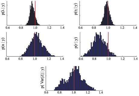
Figure 1. Parameter posterior distribution. The panels show different marginals of the posterior distribution computed using the Bayesian inference MCMC approach described in Section 3.2. For each panel, the x-axis has been rescaled to show ratios of inferred to true parameter value. The red line highlights the 1/1 ratio, which corresponds to perfectly inferred parameters. The maximum a posteriori estimates $\widehat{\gamma }$_MAP are those maximizing the posterior distribution. The parameters are λ = birth, η = death, α = immigration, r = recovery rate.

In Figure 2, the mean and variance, computed from the model using Equation (5) and γ = $\widehat{\gamma }$_MAP, are compared to the sample means and variances $\widehat{\mu }$(t_s) of the considered data set.

FIGURE 2

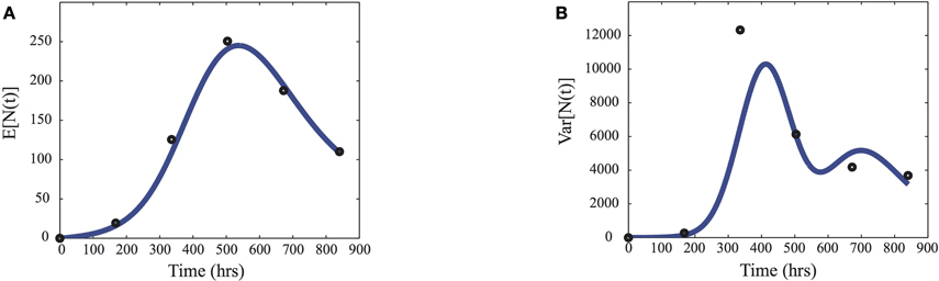
Figure 2. Inference data. Comparison of the sample means (A) and variances (B) of the pest population N(t) used to infer the parameters (dots) and the predictions given by the moment Equation (5) using the maximum a posteriori estimates $\widehat{\gamma }$_MAP given in Equation (9).

To assess the advantages of the proposed stochastic approach with respect to more standard methods based on measurements of the average species density only, we repeated the previously described inference process using only the means {$\widehat{\mu }$₁(t_s)}^S_{s = 1} as data. By comparing the parameter posterior distribution obtained in this case (Figure 3) with the one obtained using as inference data also the variance (Figure 1) one can immediately see that higher order statistics may contain valuable information regarding the parameters. As a consequence, the proposed approach could help solving identifiability problems of standard inference approaches based on deterministic models.

FIGURE 3

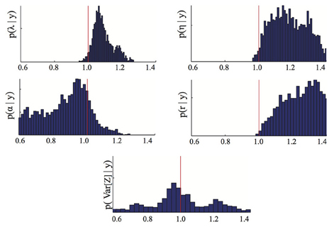
Figure 3. Parameter posterior distribution. The panels show different marginals of the posterior distribution computed using the Bayesian inference MCMC approach if only the means of the dataset D are used. For each panel, the x-axis has been rescaled to show ratios of inferred to true parameter value. The red line highlights the 1/1 ratio, which corresponds to perfectly inferred parameters. The parameters are λ = birth, η = death, α = immigration, r = recovery rate.

The previous results were obtained assuming a dataset that contains n = 100 replicates of the system for each measurement time. As rigorously encoded in the mathematical description of the noise given in Equation (6), the variance of the estimates is inversely proportional to the number of samples n. Consequently, if the number of replicates is very low, the variance of the data used in the inference may be large resulting in inconclusive (i.e., very spread) parameter posterior distributions. This is due to the fact that many different parameters give rise to model predictions that are consistent with the high level of noise given by Equation (6). To test the performance of the proposed approach for different levels of noise, we performed a case study in which we estimated the real parameter values given in Equation (8) using mean and variances estimated from different numbers of replicates. In particular, we considered four different scenarios with n = 10, n = 25, n = 50 and n = 100 replicates and simulated 10 different datasets for each scenario to reduce the influence of the particular realization of the data in the results. We then performed the parameter inference for all scenarios and all datasets (i.e., 40 times) and computed the relative error (e.g., 100 · $\frac{|\widehat{\lambda }-\lambda |}{\lambda }$) of the MAP estimates with respect to the real ones. The results are reported in Table 1. It can be seen that the precision of the estimates becomes larger as the number of replicates increases. In particular, n = 10 replicates lead to very imprecise results, whereas the estimates obtained from both n = 50 and n = 100 replicates attain reasonable precision. The scenario with n = 25 replicates provides an intermediate case and may or may not be sufficiently accurate depending on what errors are tolerable for the application.

TABLE 1

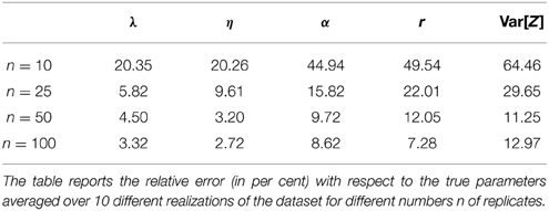
Table 1. Average error of the MAP estimates.

3.3. Optimal Control

The identified model can be used to derive optimal control strategies for pest control. Specifically, we suppose in the following that we can influence the system in Equation (7) by means of two different control strategies: pesticides and release of sterile pest individuals. While pesticides are probably the most used strategy for pest control, they present some disadvantages, as for example progressive reduction of efficiency, negative impact on beneficial insect populations (as pest natural enemies) or chemical residues in crops and in the ecosystem (Rafikov and Balthazar, 2005). For these reasons, the use of complementary or alternative biological control approaches has been suggested (Bhattacharyya and Bhattacharya, 2006; Greenman and Norman, 2007; Vreysen et al., 2007). The release of sterile insects, in particular, is a biological control method that aims at reducing the pest population size by introducing in the ecosystem sterile insects, usually male, that compete with the wild type for reproduction (Dyck et al., 2005). The desired effect is thus achieved as a result of the fact that females mating with sterile males will have no offspring. In other words sterile releases reduce the number of pest individuals available for reproduction and hence the birth rate. This approach has been successfully employed, for example, to eradicate screwworm flies, melon flies, the codling moth and pink bollworm among others, see Barclay and Li (1991) and references therein. Pesticide and sterile release are very different strategies also from an economical perspective: while the cost of pesticide is proportional to the area that has to be treated, the cost of steriles depends on the amount released. We notice that, in order to prevent a given fraction of the population from reproduction, the amount of released steriles should be roughly proportional to the number of pest individuals present in the system. Finally, the two approaches differ in the effect that they have on the ecosystem. In the following, we model the effect of pesticide as an instantaneous state reset of the pest population to N(t⁺) = (1 − u_p(t))N(t⁻), where u_p(t) ∞ [0, 1] is the percentage of the field treated with pesticide at time t. Note that since X(t) is a stochastic process, this reset influences all the moments and cross-moments of X(t) involving the random process N(t). For example, for the ith moment of N(t), that is μ^N_i(t): = 𝔼 [Nⁱ(t)], we get μ^N_i(t⁺) = (1 − u_p(t))ⁱ μ^N_i(t⁻) in Equation (5). To model the effect of the release of sterile individuals we need to include them as a new species S(t). In particular, we model the interaction between healthy and sterile individuals by

$\begin{array}{cc}\begin{array}{ccc}N+S& \stackrel{{\kappa }_1}{\to }& B\\ B& \stackrel{{\kappa }_2}{\to }& N+S\\ B+C& \stackrel{\eta }{\to }& C\\ S+C& \stackrel{\eta }{\to }& C.\end{array}& (10)\end{array}$

Note that we assume that the steriles have the same death rate as the healthy individuals, but they cannot reproduce. The interaction between the two species is modeled by assuming that each sterile individual can prevent one healthy individual from reproducing for a random time period during which both the individuals can die. Accordingly, the introduction of steriles effectively reduces the birth rate of the population. This is captured by B(t), which quantifies how many of the healthy individuals cannot reproduce at a certain time. If we denote by u_s(t) ∞ [0, 1] the percentage of steriles introduced at time t, with respect to an assumed maximal number of steriles S that can be introduced, we can again model this control action as a state reset of the extended model. Specifically, let Q(t): = u_s(t)S be the deterministic amount of steriles added at time t, then S(t⁺) = S(t⁻) + Q(t) and C(t⁺) = C(t⁻) + Q(t). Note that C(t) is updated as well since we assume that sterile individuals are also damaging the field. Again, the state reset action leads to an update of the moment equations: for example, for the moments involving only S(t), we get ${\mu }_i^S(t^{+})=E\left[S{(t^{+})}^i\right]=E\left[{(S(t^{-})+Q)}^i\right]={\displaystyle {\sum }_{h=0}^i\left(\begin{array}{c}i\\ h\end{array}\right)·{\mu }_h^S(t^{-})·Q^{i-h}}$. Overall, the effect of the two control actions is to reset the state of the extended stochastic system, leading to a hybrid model.

One of the main problems in pest management is to determine what combinations of the available treatments are most effective for maintaining the infesting population below a given economic threshold, as described in Barclay and Li (1991), (or eventually eradicating the invasion) while minimizing the economic cost. Specifically, consider a given time horizon = [0, T] and suppose that control actions can be taken at discrete time intervals t_h = hΔ_Tac where h = 1, …, H with H: = ⎿T/Δ_Tac⏌. The optimal pest management problem can be stated as the following optimization problem

$\begin{array}{cc}\begin{array}{l}\underset{\begin{array}{c}{u}_p(t_h),u_s(t_h)\\ h=1,\dots ,H\end{array}}{\min }{\displaystyle \sum _{h=1}^H[{\rho }^P{u}_p(t_h)A+{\rho }^S{u}_s(t_h)\overline{S}]}+{\rho }^C{\mu }_1^C(T)\\ \text{s}\text{.t}\text{.}P\left[N(t)>\xi \right]\le \delta ,\forall t\in \left[0,T\right],\end{array}& (11)\end{array}$

where ρ^P > 0 models the cost of pesticide per area (possibly including a disincentive to penalize the use of pesticide with respect to biological control), A is the total area of the habitat, ρ^S > 0 is the cost per sterile and ρ^C > 0 is a factor that translates the expected value of the process C at the end of the period into an economic cost due to damage to the field and hence decrement in productivity. The parameter ξ represents the economic threshold below which the pest should be contained. Note that since the considered model is stochastic it is not possible to guarantee that, for a given control strategy, all the realizations of the process will be below the economic threshold. We can however impose that the constraint should be satisfied with a given probability 1 − δ, that is, the constraint should be satisfied in 100(1 − δ)% of the realizations. In the following we assume that the average population starts below the economic threshold ξ. If this was not the case, for example due to on-going infestations, one could substitute the constraint in Equation (11) with a time-varying decreasing threshold ξ(t), which is higher at the beginning (to guarantee the feasibility of the optimization problem) and eventually reaches the desired threshold ξ.

The problem in Equation (11) is a chance constrained optimal control problem and is in general very difficult to solve (Prékopa, 1995). Some possible approaches are based on sampling techniques (Vapnik and Chervonenkis, 1971; Tempo et al., 2012; Grammatico et al., in press) or convex relaxations (see Nemirovski and Shapiro, 2006 and references therein). Here, we decided to solve a simplified version of the problem in Equation (11) by assuming that the distribution of the pest N(t) is approximately Gaussian. If this is the case, we can rewrite the constraint $P\left[N(t)>\xi \right]\le \delta$ in terms of mean and variance of the stochastic process N(t) as follows

$\begin{array}{cc}\begin{array}{l}\underset{\begin{array}{c}{u}_p(t_h),u_s(t_h)\\ h=1,\dots ,H\end{array}}{\min }{\displaystyle \sum _{h=1}^H\left[{\rho }^P{u}_p(t_h)A+{\rho }^S{u}_s(t_h)\overline{S}\right]}+{\rho }^C{\mu }_1^C(T)\\ \text{s}\text{.t}\text{.}{\mu }_1^N(t)+{\Phi }^{-1}(1-\delta )·{\sigma }^N(t)\le \xi ,\forall t\in \left[0,T\right],\end{array}& (12)\end{array}$

where Φ(·) is the cumulative distribution function of a normalized Gaussian random variable⁴ and ${\sigma }^N(t):=\sqrt{{\mu }_2^N(t)-{\mu }_1^N{(t)}^2}$ is the standard deviation of the process N(t) (Boyd and Vandenberghe, 2004, p. 157; Nemirovski and Shapiro, 2006). Note that the problem in Equation (12) depends on the moments of the stochastic processes N(t) and C(t) only. Hence it can be solved using the approximated moment equations derived in Equation (5). Given the fact that we modeled the control actions as state resets, the controlled system in Equation (5) can be thought of as a deterministic continuous-time system with discrete-time controlled jumps, leading to a hybrid optimal control problem (Branicky et al., 1998; Bensoussan and Menaldi, 2000; Shaikh and Caines, 2007).

We assume in the following that ρ^C = ρ^P = 1, ρ^S = 4, S = 200, and A = 100. Figure 4 reports the result of the optimization problem, solved using the function fmincon of Matlab, for δ = 0.1, a horizon of 6 weeks, Δ_Tac = 1 week and deterministic initial state N(0) = C(0) = 10. The lowest possible economic threshold that guarantees feasibility of the problem in Equation (12), given the chosen initial condition and the fact that the first intervention is after 1 week, is 130. For the results of Figure 4, we fixed ξ = 150. To find the global minimum of the non-convex problem in Equation (12) we restarted the optimization from 10 different random initial control vectors and then selected the strategy with minimum cost. For solving the moment equations in Equation (12), we used the identified parameters $\widehat{\gamma }$_MAP given in Equation (9) and we set the unknown parameters κ₁ = κ₂ = 0.01. The resulting optimal control laws, u^⋆_p, u^⋆_s, consist of applying pesticide to almost all the crop field at the first possible control time t₁ = 168 hrs and subsequently controlling the population with consecutive sterile releases. This result is consistent with the analysis reported in Barclay and Li (1991), where it was shown that releasing steriles is economically preferable when the infesting population is low, while if the population is high, pesticide has to be preferred.

FIGURE 4

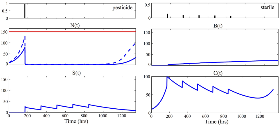
Figure 4. Optimal control strategy. The two panels at the top visualize the optimal control strategy u^⋆_p, u^⋆_s, solution of Equation (12). For all the other panels, the solid blue line represents the time evolution of the mean of the corresponding process, [respectively, N(t), S(t), B(t), and C(t)], according to the optimal control laws. To obtain these results we solved the approximated moment Equations (5) using the identified parameters $\widehat{\gamma }$_MAP, given in Equation (9), together with κ₁ = κ₂ = 0.01. In the plot of the healthy population N(t), the dashed line represents the quantity μ^N₁(t) + Φ⁻¹(0.9) · σ^N(t). The fact that this line is below the economic threshold ξ = 150 (red line) guarantees that the constraint of the problem in Equation (12) is satisfied. Consequently the stochastic realizations of the pest population are contained below the economic threshold, that is N(t) < ξ, with probability 100(1-δ) = 90%.

In order to test the performance of the derived control law, we simulated the behavior of the model in Equations (7) and (10), according to the real parameters given in Equation (8), using the stochastic simulation algorithm. Specifically, we performed 500 simulations and reported in Figure 5 the median (blue line) and the probability distribution of N(t) and C(t). Figure 5A illustrates the behavior of the system if no control action is taken. We see that in this case the pest population exceeds the economical threshold ξ = 150. In Figure 5B, on the other hand, we see that the computed optimal control laws u^⋆_p, u^⋆_s successfully regulate all the possible realizations, maintaining the population well-under the given threshold. This result is obtained by applying pesticide at time t₁ = 168 h and then using only sterile release. To show that a single application of pesticide at the beginning of the horizon would not suffice to control the population, we show in Figure 5C the behavior of the system if only the optimal control law u^⋆_p is applied. From the result it appears that the use of steriles is fundamental to complement the effect obtained by applying u^⋆_p.

FIGURE 5

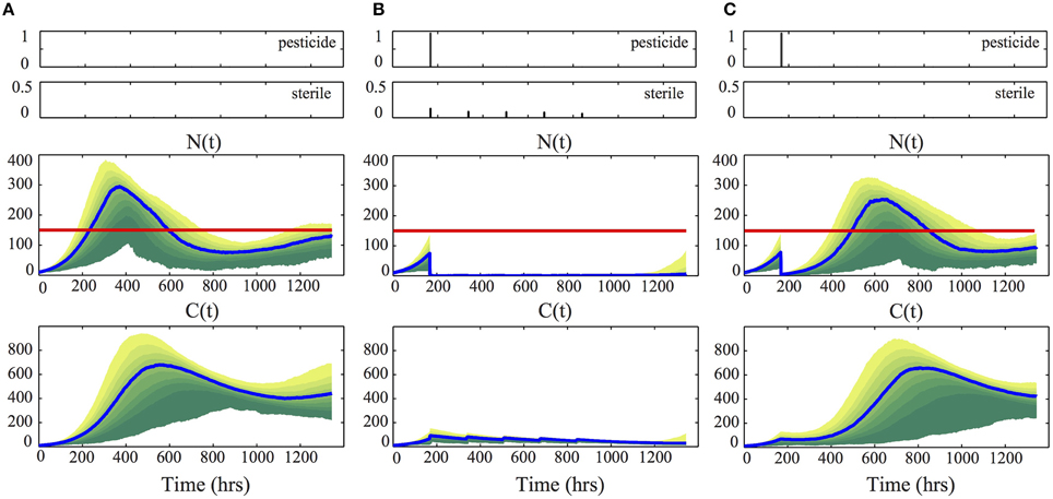
Figure 5. Control performances. For each column, the performance of the control strategy shown at the top is illustrated. Specifically, the middle and bottom panels visualize the probability distribution of N(t) and C(t), obtained from 500 stochastic simulations, using the real parameters given in Equation (8) and κ₁ = κ₂ = 0.01. The blue line denotes the median of the distribution (i.e., 50% of the realizations are below this line), the nested colored regions represent the cumulative distribution of N(t) and C(t), with steps of 10% (i.e., 10% of the realizations are inside the dark green region and 90% are inside the yellow one). The red line represent the economical threshold ξ = 150. (A) refers to no control action, (B) to the optimal strategy u^⋆_p, u^⋆_s, and (C) to the use of u^⋆_p, only.

4. Discussion

One of the major future challenges for ecologists is to find strategies for organizing human interactions with the environment in a long-term sustainable way. We believe that dynamical models, inferred from measured data, together with optimal control theory have the potential to be of substantial help in achieving this task. While it is usually straightforward to incorporate the effect of human actions in a model and to formulate related optimal control problems, solving these problems may be a challenge. This has however not prevented the advancement of control theory across all engineering disciplines. So why is it that optimal control has not found more applications in ecology? A reason for this is the intrinsic complexity of ecological systems. Contrary to engineering disciplines, where the systems usually have known structure and parameters, ecological systems have been shaped by evolution in ways that we do not yet fully understand. Therefore, before we can attempt to control an ecological system with the help of a mathematical model, we first need to identify an appropriate model and its parameters from measured field data. This task is complicated by the fact that ecological systems are inherently driven by random interactions between individuals that take place in spatially structured habitats and may be influenced by different environmental conditions. To be applicable in practice, a model should take into account all these factors.

In this paper, we took a first step in this direction by proposing an approach for dealing with stochasticity and varying environmental conditions, neglecting the spatial aspect of the problem. Our approach requires data from many different replicates of the system. In the current paper we used a simulated dataset; as future work it is important to test this method on real data. These may not be straightforward to obtain in some applications, as for the pest control application considered here. However, one could envision grouping a habitat into many small and clearly separated patches. Each patch could then provide a replicate of the system. Another possibility would be to “zoom out” and regard the model not as a model for one specific habitat (i.e., one specific crop), but as a model for all habitats of this kind (i.e., all cotton crops), for instance in an entire country. Based on the identified model, we formulated an optimal control problem in which two different control strategies can be used to reduce the pest population, both resulting in a state reset. This lead to a hybrid system in which the control operator can reset the state at certain given intervention times, while the dynamics of the system between the reset times are given by a continuous-time stochastic process.

All of the results of this paper rely on the possibility to obtain good approximations of the moments of the species abundances, that is, on the existence of an adequate moment closure method for the studied system. In some applications, it can happen that all the available methods do not perform adequately. To address this issue, further work is required on the development of new moment closure methods. From a hybrid systems perspective, an appealing approach is to group the interacting species into highly and lowly abundant species and to model them using continuous deterministic and discrete stochastic dynamics, respectively. Methods to analyze such hybrid models have been developed recently (Jahnke, 2011), but their use for parameter inference or optimal control has so far not been documented.

Author Contributions

FP and JR designed and performed the research. All authors wrote the paper.

Funding

The research leading to these results has received funding from the People Programme (Marie Curie Actions) of the European Union's Seventh Framework Programme (FP7/2007-2013) under REA grant agreement No. [291734] and from SystemsX under the project SignalX.

Conflict of Interest Statement

The authors declare that the research was conducted in the absence of any commercial or financial relationships that could be construed as a potential conflict of interest.

Acknowledgments

The authors would like to acknowledge contributions from Baptiste Mottet who performed preliminary analysis regarding parameter inference for the considered case study in a student project (Mottet, 2014/2015).

Footnotes

1. ^Extension to multiple measured species is straightforward.

2. ^The assumption that n is the same for each time point is only for notational convenience and is by no means necessary.

3. ^For ease of notation we omit the dependence of this probability on the initial condition.

4. ^If no information is known about the distribution, Chebyshev's inequality can be used to enforce the constraint P[ N(t) > ξ] ≤ δ, leading to the more restrictive bound ${\mu }_1^N(t)+\sqrt{\frac{1}{\delta }}·{\sigma }^N(t)\le \xi$.

References

Altermatt, F., Fronhofer, E. A., Garnier, A., Giometto, A., Hammes, F., Klecka, J., et al. (2014). Big answers from small worlds: a user's guide for protist microcosms as a model system in ecology and evolution. Methods Ecol. Evol. 6, 218–231. doi: 10.1111/2041-210X.12312

CrossRef Full Text | Google Scholar

Balazsi, G., van Oudenaarden, A., and Collins, J. (2011). Cellular decision making and biological noise: from microbes to mammals. Cell 144, 910–925. doi: 10.1016/j.cell.2011.01.030

PubMed Abstract | CrossRef Full Text | Google Scholar

Barclay, H. J., and Li, C. (1991). Combining methods of pest control: minimizing cost during the control program. Theor. Popul. Biol. 40, 105–123.

Google Scholar

Bensoussan, A., and Menaldi, J. L. (2000). Stochastic hybrid control. J. Math. Anal. Appl. 249, 261–288. doi: 10.1006/jmaa.2000.7102

CrossRef Full Text | Google Scholar

Bhattacharyya, S., and Bhattacharya, D. (2006). Pest control through viral disease: mathematical modeling and analysis. J. Theor. Biol. 238, 177–197. doi: 10.1016/j.jtbi.2005.05.019

PubMed Abstract | CrossRef Full Text | Google Scholar

Black, A., and McKane, A. (2012). Stochastic formulation of ecological models and their applications. Trends Ecol. Evol. 27, 337–345. doi: 10.1016/j.tree.2012.01.014

PubMed Abstract | CrossRef Full Text | Google Scholar

Boyd, S., and Vandenberghe, L. (2004). Convex Optimization. Cambridge, UK: Cambridge University Press.

Google Scholar

Branicky, M. S., Borkar, V. S., and Mitter, S. K. (1998). A unified framework for hybrid control: model and optimal control theory. IEEE Trans. Automat. Control 43, 31–45.

Google Scholar

Carrara, F., Giometto, A., Seymour, M., Rinaldo, A., and Altermatt, F. (2014). Experimental evidence for strong stabilizing forces at high functional diversity of aquatic microbial communities. Ecology 96, 1340–1350. doi: 10.1890/14-1324.1

CrossRef Full Text | Google Scholar

Cordero, O., Ventouras, L., DeLong, E., and Polz, M. (2012). Public good dynamics drive evolution of iron acquisition strategies in natural bacterioplankton populations. Proc. Natl. Acad. Sci. U.S.A. 109, 20059–20064. doi: 10.1073/pnas.1213344109

PubMed Abstract | CrossRef Full Text | Google Scholar

DeAngelis, D. L., and Mooij, W. M. (2005). Individual-based modeling of ecological and evolutionary processes. Annu. Rev. Ecol. Evol. Syst. 36, 147–168. doi: 10.1146/annurev.ecolsys.36.102003.152644

CrossRef Full Text | Google Scholar

Dyck, V. A., Hendrichs, J., and Robinson, A. S. (2005). Sterile Insect Technique. Dordrecht: Springer.

Google Scholar

Gillespie, C., and Golightly, A. (2010). Bayesian inference for generalized stochastic population growth models with application to aphids. J. R. Stat. Soc. C 59, 341–357. doi: 10.1111/j.1467-9876.2009.00696.x

CrossRef Full Text | Google Scholar

Gillespie, D. (1976). A general method for numerically simulating the stochastic time evolution of coupled chemical reactions. J. Comput. Phys. 22, 403–434. doi: 10.1016/0021-9991(76)90041-3

CrossRef Full Text | Google Scholar

Goutsias, J., and Jenkinson, G. (2013). Markovian dynamics on complex reaction networks. Phys. Rep. 529, 199–264. doi: 10.1016/j.physrep.2013.03.004

CrossRef Full Text | Google Scholar

Grammatico, S., Zhang, X., Margellos, K., Goulart, P., and Lygeros, J. (in press). A scenario approach for non-convex control design. IEEE Trans. Automat. Control. doi: 10.1109/TAC.2015.2433591

CrossRef Full Text | Google Scholar

Greenman, J. V., and Norman, R. A. (2007). Environmental forcing, invasion and control of ecological and epidemiological systems. J. Theor. Biol. 247, 492–506. doi: 10.1016/j.jtbi.2007.03.031

PubMed Abstract | CrossRef Full Text | Google Scholar

Hekstra, D. R., and Leibler, S. (2012). Contingency and statistical laws in replicate microbial closed ecosystems. Cell 149, 1164–1173. doi: 10.1016/j.cell.2012.03.040

PubMed Abstract | CrossRef Full Text | Google Scholar

Hespanha, J. (2008). “Moment closure for biochemical networks,” in 3rd International Symposium on Communications, Control and Signal Processing (St Julians), 142–147.

Google Scholar

Isham, V. (1991). Assessing the variability of stochastic epidemics. Math. Biosci. 107, 209–224. doi: 10.1016/0025-5564(91)90005-4

PubMed Abstract | CrossRef Full Text | Google Scholar

Jahnke, T. (2011). On reduced models for the chemical master equation. Multiscale Model. Simul. 9, 1646–1676. doi: 10.1137/110821500

CrossRef Full Text | Google Scholar

Jaquette, D. (1970). A stochastic model for the optimal control of epidemics and pest populations. Math. Biosci. 8, 343–354.

Google Scholar

Krishnarajah, I., Cook, A., Marion, G., and Gibson, G. (2005). Novel moment closure approximations in stochastic epidemics. Theor. Popul. Biol. 67, 855–873. doi: 10.1016/j.bulm.2004.11.002

PubMed Abstract | CrossRef Full Text | Google Scholar

Kügler, P. (2012). Moment fitting for parameter inference in repeatedly and partially observed stochastic biological models. PLOS ONE 7:e43001. doi: 10.1371/journal.pone.0043001

PubMed Abstract | CrossRef Full Text | Google Scholar

Lagarrigues, G., Jabot, F., Lafond, V., and Courbaud, B. (2014). Approximate Bayesian computation to recalibrate individual-based models with population data: illustration with a forest simulation model. Ecol. Modell. 306, 278–286. doi: 10.1016/j.ecolmodel.2014.09.023

CrossRef Full Text | Google Scholar

Lavielle, M. (2014). Mixed Effects Models for the Population Approach: Models, Tasks, Methods and Tools. Boca Raton, FL: Chapman & Hall; CRC.

Google Scholar

Marion, G., Renshaw, E., and Gibson, G. (1998). Stochastic effects in a model of nematode infection in ruminants. Math. Med. Biol. 15, 97–116. doi: 10.1093/imammb/15.2.97

PubMed Abstract | CrossRef Full Text | Google Scholar

Matis, J., Kiffe, T., Matis, T., and Stevenson, D. (2007). Stochastic modeling of aphid population growth with nonlinear power-law dynamics. Math. Biosci. 208, 469–494. doi: 10.1016/j.mbs.2006.11.004

PubMed Abstract | CrossRef Full Text | Google Scholar

McKinley, T., Cook, A., and Deardon, R. (2009). Inference in epidemic models without likelihoods. Int. J. Biostat. 5, 24. doi: 10.2202/1557-4679.1171

PubMed Abstract | CrossRef Full Text | Google Scholar

Milner, P., Gillespie, C., and Wilkinson, D. (2013). Moment closure based parameter inference of stochastic kinetic models. Stat. Comput. 23, 287–295. doi: 10.1007/s11222-011-9310-8

CrossRef Full Text | Google Scholar

Mottet, B. Q. (2014/2015). Application of Moment-Based Methods for Parameter Inference to Nonlinear Stochastic Population Growth Model. Technical Report, Semester Project, ETH Zurich. Supervisors: F. Parise, J. Ruess, and J. Lygeros.

Munsky, B., and Khammash, M. (2006). The finite state projection algorithm for the solution of the chemical master equation. J. Chem. Phys. 124:044104. doi: 10.1063/1.2145882

PubMed Abstract | CrossRef Full Text | Google Scholar

Murray, J. D. (2002). “Mathematical biology I. An introduction,” in Interdisciplinary Applied Mathematics, Vol. 17, eds S. S. Antman, J. E. Marsden, L. Sirovich, and S. Wiggins (New York, NY: Springer), 1–537.

Nemirovski, A., and Shapiro, A. (2006). Convex approximations of chance constrained programs. SIAM J. Optimiz. 17, 969–996. doi: 10.1137/050622328

CrossRef Full Text | Google Scholar

Neuert, G., Munsky, B., Tan, R., Teytelman, L., Khammash, M., and van Oudenaarden, A. (2013). Systematic identification of signal-activated stochastic gene regulation. Science 339, 584–587. doi: 10.1126/science.1231456

PubMed Abstract | CrossRef Full Text | Google Scholar

Nåsell, I. (2002). Stochastic models of some endemic infections. Math. Biosci. 179, 1–19. doi: 10.1016/S0025-5564(02)00098-6

PubMed Abstract | CrossRef Full Text | Google Scholar

Nåsell, I. (2003). Moment closure and the stochastic logistic model. Theor. Popul. Biol. 63, 159–168. doi: 10.1016/S0040-5809(02)00060-6

PubMed Abstract | CrossRef Full Text | Google Scholar

Ovaskainen, O., and Cornell, S. (2006). Space and stochasticity in population dynamics. Proc. Natl. Acad. Sci. U.S.A. 103, 12781–12786. doi: 10.1073/pnas.0603994103

PubMed Abstract | CrossRef Full Text | Google Scholar

Ovaskainen, O., and Meerson, B. (2010). Stochastic models of population extinction. Trends Ecol. Evol. 25, 643–652. doi: 10.1016/j.tree.2010.07.009

PubMed Abstract | CrossRef Full Text | Google Scholar

Poovathingal, S., and Gunawan, R. (2010). Global parameter estimation methods for stochastic biochemical systems. BMC Bioinformatics 11:414. doi: 10.1186/1471-2105-11-414

PubMed Abstract | CrossRef Full Text | Google Scholar

Prékopa, A. (1995). Stochastic Programming. Dordrecht: Kluwer Academic Publishers.

Rafikov, M., and Balthazar, J. M. (2005). Optimal pest control problem in population dynamics. Comput. Appl. Math. 24, 65–81. doi: 10.1590/S1807-03022005000100004

CrossRef Full Text | Google Scholar

Railsback, S., and Grimm, V. (2012). “Individual-based ecology,” in Encyclopedia of Theoretical Ecology, eds A. Hastings and L. J. Gross (Berkeley: University of California Press), 365–370.

Ross, J., Pagendam, D., and Pollett, P. (2009). On parameter estimation in population models II: multi-dimensional processes and transient dynamics. Theor. Popul. Biol. 75, 123–132. doi: 10.1016/j.tpb.2008.12.002

PubMed Abstract | CrossRef Full Text | Google Scholar

Ruess, J., and Lygeros, J. (2013). “Identifying stochastic biochemical networks from single-cell population experiments: a comparison of approaches based on the Fisher information,” in IEEE 52nd Annual Conference on Decision and Control (CDC) (Florence), 2703–2708.

Google Scholar

Ruess, J., and Lygeros, J. (2015). Moment-based methods for parameter inference and experiment design for stochastic biochemical reaction networks. ACM Trans. Model. Comput. Simul. 25:8. doi: 10.1145/2688906

CrossRef Full Text | Google Scholar

Ruess, J., Milias-Argeitis, A., and Lygeros, J. (2013). Designing experiments to understand the variability in biochemical reaction networks. J. R. Soc. Interface 10:20130588. doi: 10.1098/rsif.2013.0588

PubMed Abstract | CrossRef Full Text | Google Scholar

Ruess, J., Milias-Argeitis, A., Summers, S., and Lygeros, J. (2011). Moment estimation for chemically reacting systems by extended Kalman filtering. J. Chem. Phys. 135:165102. doi: 10.1063/1.3654135

PubMed Abstract | CrossRef Full Text | Google Scholar

Shahid Shaikh, M., and Caines, P. E. (2007). On the hybrid optimal control problem: theory and algorithms. IEEE Trans. Automat. Control 52, 1587–1603. doi: 10.1109/TAC.2007.904451

CrossRef Full Text | Google Scholar

Singh, A., and Hespanha, J. (2006). “Lognormal moment closures for biochemical reactions,” in 45th IEEE Conference on Decision and Control (San Diego, CA), 2063–2068. doi: 10.1109/CDC.2006.376994

CrossRef Full Text | Google Scholar

Srivastava, D. S., Kolasa, J., Bengtsson, J., Gonzalez, A., Lawler, S. P., Miller, T. E. et al. (2004). Are natural microcosms useful model systems for ecology? Trends Ecol. Evol. 19, 379–384. doi: 10.1016/j.tree.2004.04.010

PubMed Abstract | CrossRef Full Text | Google Scholar

Stumpf, M. (2014). Approximate Bayesian inference for complex ecosystems. F1000Prime Rep. 6:60. doi: 10.12703/P6-60

PubMed Abstract | CrossRef Full Text | Google Scholar

Tempo, R., Calafiore, G., and Dabbene, F. (2012). Randomized Algorithms for Analysis and Control of Uncertain Systems: With Applications. London: Springer Science & Business Media.

Google Scholar

Toni, T., Welch, D., Strelkowa, V., Ipsen, A., and Stumpf, M. (2009). Approximate Bayesian computation scheme for parameter inference and model selection in dynamical systems. J. R. Soc. Interface 6, 187–202. doi: 10.1098/rsif.2008.0172

PubMed Abstract | CrossRef Full Text | Google Scholar

Vapnik, V. N., and Chervonenkis, A. Y. (1971). On the uniform convergence of relative frequencies of events to their probabilities. Theory Probab. Appl. 16, 264–280.

Google Scholar

Vreysen, M. J., Robinson, A., and Hendrichs, J. (2007). Area-wide Control of Insect Pests: From Research to Field Implementation. Dordrecht: Springer Science & Business Media.

Google Scholar

Whittle, P. (1957). On the use of the normal approximation in the treatment of stochastic processes. J. R. Stat. Soc. B 19, 268–281.

Google Scholar

Wickwire, K. (1977). Mathematical models for the control of pests and infectious diseases: a survey. Theor. Popul. Biol. 11, 182–238.

PubMed Abstract | Google Scholar

Wolf, V., Goel, R., Mateescu, M., and Henzinger, T. (2010). Solving the chemical master equation using sliding windows. BMC Syst. Biol. 4:42. doi: 10.1186/1752-0509-4-42

PubMed Abstract | CrossRef Full Text | Google Scholar

Zechner, C., Ruess, J., Krenn, P., Pelet, S., Peter, M., Lygeros, J., et al. (2012). Moment-based inference predicts bimodality in transient gene expression. Proc. Natl. Acad. Sci. U.S.A. 109, 8340–8345. doi: 10.1073/pnas.1200161109

PubMed Abstract | CrossRef Full Text | Google Scholar