Atmospheric CO2 fertilization effects on biomass yields of 10 crops in northern Germany

1. Introduction

Ever since the 1970s plant and crop scientists have undertaken attempts to quantify the effects of atmospheric carbon dioxide [CO₂] concentrations on the development of plants (Fleisher et al., 2011). Since then basically two mechanisms have emerged that might have critical implications for crop yields if [CO₂] concentrations are changed.

One is an elevated photosynthesis rate, resulting in more energy and thus a quicker development of the plant. In a stricter sense this is often the effect meant when implicating a [CO₂] fertilization effect. C₃-plants like wheat, rice or barley interact directly with [CO₂] for their photosynthesis and are thus more susceptible to concentration changes in the ambient air. It is commonly expected that these plants will increasingly benefit from elevated photosynthesis rates up to around 1000 ppm [CO₂], more than twice the concentration of today's atmosphere. C₄ plants like maize, sorghum or sugarcane are however, comparatively independent of changes in [CO₂]. Their photosynthesis rate does increase similar to C₃-plants toward today's [CO₂] concentration, then, however, starts to quickly level out around 400 ppm (Ehleringer and Cerling, 2002; Chmielewski, 2007; Lambers et al., 2008).

On the other hand an increase in [CO₂] reduces the amount of water needed to produce an equivalent amount of biomass. This improvement in water use efficiency (WUE) is due to a closing of the stomata to regulate the flux of [CO₂] molecules and affects both C₃- and C₄-plants alike. More or less as a byproduct, these more narrow stomata restrict the amount of H₂O molecules that are transpired by the plant (Steffen and Canadell, 2005; Lambers et al., 2008).

Some discrepancies about the quantity of both effects arose when FACE (Free-Air-CO₂ Enrichment) studies emerged during the 1990s, as prior knowledge on [CO₂] fertilization effects was based entirely on experiments in growing chambers. FACE experiments are situated in open air, within the natural atmosphere. [CO₂] is emitted through tubes around the plant samples and regulated to the desired level (Kimball et al., 2002; Kimball, 2011). Tests in secluded SPAR (Soil-Plant-Atmosphere-Research) chambers produce results that mostly surpassed those in FACE experiments under near natural conditions. The advantage of such chamber tests is an extensive control of all parameters within the chamber (Fleisher et al., 2011). The diverging results in biomass yields, grain yields or photosynthesis rate, however, suggest that not all natural processes are reproduced satisfactorily within these secluded environments.

As an example, tests with some C₃-plants did show an increase in biomass and grain yields by 17% and 13%, respectively. This was done in FACE tests at 25°C and 550 ppm [CO₂]. These yields are only about half of those from comparable chamber tests. C₄-plants did not show any increase at all (Long et al., 2006). However, those studies are generally hard to compare. FACE studies, done since 1989, are still relatively rare in comparison to chamber tests, as they require considerably more resources to conduct. Those studies available often use different conditions, most importantly different [CO₂] concentrations. The matter becomes even more complex when the plant's supply of nutritional elements (e.g. N), water supply and temperature as well as their interaction are considered, as they have a major impact on the final result. If, for example, the water availability is accounted for, even C₄-plants are then affected by an elevated [CO₂], as they do not react under normal or optimal conditions to more [CO₂] but do so if their water supply is limited (Kimball, 2011).

Some authors (Morgan et al., 2004) even suggest that the indirect water saving aspect of elevated [CO₂] levels might outperform the direct effect of increased photosynthesis rates, especially under increasingly dry conditions due to climatic changes. Apparently, this effect can be so strong that even under conditions of increasing summer drought stress, when one would normally expect declining yields, some Grasslands still gained in yields due to a rise in [CO₂] (Taube and Herrmann, 2009).

To date, no comprehensive approach exists that would represent all related aspects and interactions within a single modeling environment. In any case the uncertainties concerning crop yields seem to be relatively large today. As many models use the results from SPAR and similar experiments to quantify the role of [CO₂] in plant growth, it might be the case that studies conducted using these models over-estimate future yields. It is further suggested that the variability in yields due to [CO₂] responses is almost as large as those caused by climate interactions (McGrath and Lobell, 2013). While global studies on crop yields might be relatively robust in regard to this variability, it might have a larger impact at regional scales. However, regional disparities in the context of climate and crops are not well understood and studies concerning this topic are relatively sparse today (Rosenthal and Tomeo, 2013).

A regional study in this regard was done in Germany by Huang et al. (2012) at two catchments for winter wheat. Their results suggested that a decrease in yields by the mid-twenty-first century of 6–10% due to a negative change in water availability, reverses into an increase of 9–14% when [CO₂] fertilization effects are included. A similar study by Kersebaum and Nendel (2014), also for winter wheat and varying sites in Germany, using the same climate model and scenario as the presented study, reported yield decreases by -11.6% if the effect was neglected and depending on the algorithm (three tested in total), 0.9 to 6.0% yield increases if the [CO₂] effect was included. Apart from this, several articles exist that deal with [CO₂] and crop yields on different scales and approaches (Ziska and Bunce, 2007; Högy and Fangmeier, 2008; Soussana et al., 2010; Vanuytrecht et al., 2011; Weigel and Manderscheid, 2012; Tausz et al., 2013; Wang et al., 2013).

This study aims at extending this knowledge by estimating the influence an elevated [CO₂] concentration has on the biomass yields of 10 different crops throughout the twenty-first century in the area of Niedersachsen, Germany. This is done site specific to capture interactions between species, [CO₂], temperature, precipitation and different soils. The mentioned abiotic influences serve as input variables for the BioSTAR crop model that calculates annual biomass yields. To estimate the strength of the [CO₂] signal on the resulting yields, two separate runs were conducted: (I) all climate variables are changed annually according to the used climate model data including [CO₂] and (II) all climate variables are changed annually according to the used climate model data except for [CO₂] which is kept at 390 ppm. The difference of both runs is then used to estimate the quantitative [CO₂] influence (i.e., is there a measurable effect at all and how strong is it?) and to determine its quality (i.e., is it the photosynthesis or the water saving aspect that is the main responsible factor). The strength and significance of all abiotic input variables are estimated using a multivariate linear regression model. The results will be assessed in general for the entire research area as well as site-specific.

2. Materials and Methods

Basically climate and soil data were combined within a crop model to estimate biomass yields. Modeling was done for each crop and each year individually, once with an adapted [CO₂] concentration and once with fixed 390 ppm. The modeling with the fixed [CO₂] concentration should be seen as a hypothetical framework to distinguish the [CO₂] influence signal on yields from that of the other input variables. It should not reflect an actual future climate development. Results are given as relative to today, whereas today refers to the period 2001-2010. All involved components are discussed in detail below.

2.1. Area of Interest: Niedersachsen

Niedersachsen (NI) constitutes a land area of about 46,500 km² and is thus the second largest of all 16 federal states in Germany, providing roughly 1/6 of the national agricultural land (DeStatis, 2013). Located to the North-West of Germany (Figure 1), the state lies in a transition zone between a more maritime (NW) toward a more continental climate (SE) (Seedorf and Meyer, 1992) with an average annual temperature of around 9°C and a mean precipitation of 749 mm in the period of 1971–2000 (DWD, 2014).

FIGURE 1

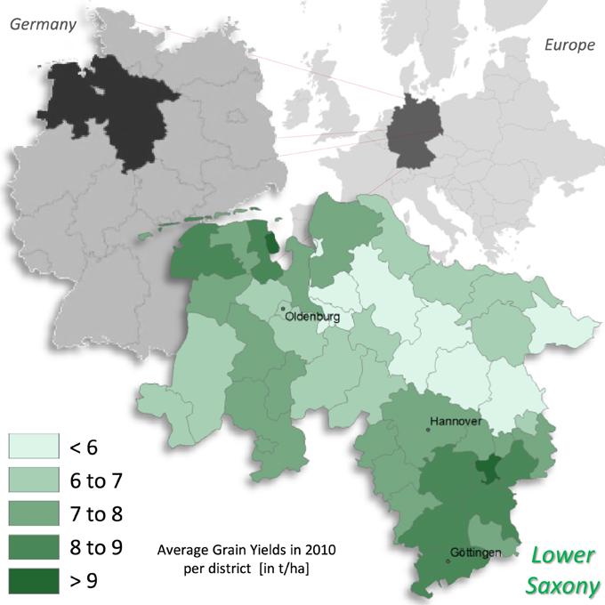
Figure 1. The Research Area Niedersachsen. Displayed are the average yields of all grains for the year 2010 by district in t/ha (LSN, 2014).

NI can be subdivided into three major landscape structures: the coast, including the East Frisian Islands, the German North-Western Lowland (amounting for three quarters of NI overall land area) as well as a low mountain range to its south, with the Harz as its most prominent member (Drachenfels, 2010).

The broad loess valleys to the south and especially the fertile “Börde” that fronts the low mountain range to the north are the main cultivation areas for high-demand crops like winter wheat. Here, average grain yields are generally above 8 t/ha, though dropping below 6 t/ha in the northern Lowland, mainly consisting of “Geest”-land, quaternary sediments that are particularly sandy to the North-East, with precipitation as low as 500 mm, making irrigation already today necessary on several sites. The west of NI is dominated by livestock farming with the coastal area predominantly used for grassland farming as high ground water levels prevent intensive agricultural use. On those sites where intensive agriculture is feasible the grain yields reach levels comparable to the very good soils in Niedersachsen's south-east (Heunisch et al., 2007).

2.2. Crop Model

The crop model used for the modeling of biomass was BIOSTAR, recently developed at the Georg-August-University in Göttingen (Bauböck, 2013). The model was chosen for this study mostly for its carbon-based growth engine but also due to the fact that it was developed and validated on sites in Niedersachsen and can be used on a large number of sites. The local validation increased the confidence in the results, as no cross-checking for model biases due to change in geographic location was necessary. Even more important, the carbon-based growth engine allowed to explicitly take [CO₂] fertilization effects into account.

Model validation was performed using data from two test sites of the Chamber of Agriculture: Poppenburg and Werlte. Data on actual yields were available between 2006 and 2010. Deviations between measured and modeled data were calculated as the Root Mean Square Error (RMSE). The %-error values $\left(\frac{RSME}{measured mean}\times 100\right)$ in Table 1 show that the difference in measured and modeled yields is generally below 10% and the model is thus expected to represent the reality of yields in Niedersachsen reasonably well (Bauböck, 2013).

TABLE 1

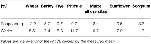
Table 1. Validation of the BioSTAR crop model with measured data at two test sites.

The model requires precipitation, temperature, [CO₂], solar radiation, relative air humidity and wind-speed at 2 m altitude to compute yields. As the model was originally conceived to estimate bio-energy potentials, the primary computation product is the crop's biomass.

To estimate the [CO₂] influence the model uses equations taken from an 1995 article from Hoffmann (1995) that were used to describe photosynthesis rates in beeches. These were constructed in accordance to the Michaelis–Menten Theory and originally described by Gaastra (1959) to assess photosynthesis rates of sugar beet. However, HOFFMANN expects due to further testing that the presented results hold true for other C₃-plants as well.

In a comparison of several different approaches to determine photosynthesis rates in C₃-plants against actual results from FACE experiments (Nendel et al., 2009), the approach suggested by HOFFMANN did show the best results when estimating dry matter, yield, LAI and soil moisture changes.

The plants water consumption is calculated by BioSTAR using fluxes between the leaf and atmosphere, using the water vapor gradient and CO₂ concentrations within the leaf. All related equations and further discussions of model parameters have been published by the model's developer (Bauböck, 2013, 2014).

Within the scope of all known uncertainties, it is therefore expected that the BioSTAR crop model can adequately represent biomass yield changes due to changes in [CO₂].

All in all ten different crops are included in this study. These crops are the winter grains wheat, barley, rye and triticale, an early, medium and late maize variety as well as sunflower, sorghum and spring wheat. These crops were chosen simply because they were already available and validated at the time this study was conducted. The late maize variety and sorghum are currently not part of the crop rotation in NI, as local temperatures are not sufficient yet. No adaptation of sowing date due to climate change was applied and all plants were modeled until full maturity.

2.3. Soil Data

The soil data in this study were derived from the official digital soil survey map of Niedersachsen in a resolution of 1 : 50,000, labeled BÜK 50 (Boess et al., 2004). This map was intersected with data from the CORINE land-use classification of 2005 for Niedersachsen to extract sites that are used for agricultural purposes. The result between the intersected soil and land-use map was a data-set of 91,014 sites where each was used for a unique modeling run. The soil map contained codified information on the soil type and its thickness that were translated into the format required by BioSTAR. Fifteen 10 cm soil levels had to be identified, each containing the information on prevalent soil type with a 16th level representing everything below these initial 1.5 m. The crop model uses this information for the calculation of soil water content and flows (Bauböck, 2014).

2.4. Climate Model and Data

The regional climate model used for this study is WETTREG, a German portmanteau word translating into “weather condition-based regional model.” The model is developed by the “Climate & Environment Consulting Potsdam GmbH” on behalf of several German state authorities and uses a statistical downscaling method. Large scale atmospheric patterns are statistically connected with data from local climate stations. An initial link is created between measured data at these stations and globally gridded reanalysis data, using both ERA 40 and NCEP/NCAR data. This link is then reestablished through GCM-derived gridded data of a future climate. In this case, data from the ECHAM 5 global climate model came to use. For each large scale weather pattern of the future, a pool of local station data is available that is then resampled several times to create the climate signal (Enke and Spekat, 1997; Enke et al., 2005). The model's actual name is WETTREG 2010, as the initial approach (today labeled WETTREG 2006) neglected atmospheric patterns that are relatively rare as of today but will increasingly emerge under a future climate. Thus, two patterns were added to this latest version, significantly reducing the model bias in comparison to other climate models (Kreienkamp et al., 2010).

The data was provided by the State Authority for Mining, Energy and Geology (LBEG), where WETTREG 2010 was applied at 248 stations distributed throughout NI, whereas the mean of 10 iterations at each station was used as the climate signal for the twenty-first century (A1B SRES scenario). Using spatial interpolation methodology, these point-based information were further downscaled to a grid of 100×100 m at the Jülich Research Centre through the CLINT interpolation model (Müller et al., 2012). This resulted in a grid of 11,520,000 data points for each time step (with 10-day-values amounting to 36 single steps per year) for Temperature, Precipitation and Potential Evapotranspiration. The data was available for the years 1961–2100 with an additional data-set of interpolated measured station data from Germany's National Meteorological Service (DWD) for the years 1961–2005 for validation purposes. The climate data-sets agreed reasonably well in temperature and precipitation (with WETTREG2010 showing a mean annual average bias of +0.02°C and −2.24% precipitation in the period 1971–2000). Especially this precipitation bias is about the same magnitude as the projected precipitation changes during the twenty-first century, at least in its first half.

Further data on Global Radiation was taken from a run of ECHAM 5 in a global T31 grid of 48 × 96 that was calculated within the scope of the ENSEMBLES project (Roeckner, 2009). The ECHAM 5 data was chosen for the purpose of data consistency as the WETTREG2010 data did also employ ECHAM 5 runs for its boundary conditions. The data-set was provided for the years 2001 until 2099, thus setting the limits for this study's time-frame. Global radiation was calculated as the sum of surface net downward shortwave flux and surface net downward longwave flux.

Wind Speed was taken from official maps of NI of 2005 provided through the State Authority for Mining, Energy and Geology (LBEG) that uses the FAO approach for wind speed at a height of 2 m above grass. Typical wind speed ranges from 5 to 6 m/s in coastal areas to around 1–2 m/s in the south of NI. To present knowledge, no significant change in the wind speed pattern is anticipated for the future (NMUEK, 2012); hence, the data was applied without further changes.

Relative Air Humidity was calculated backwards from the WETTREG2010 data on evapotranspiration, as this was derived through the Penman-Monteith approach.

All of the above mentioned data was then intersected with the soil sites using the respective variables mean value.

[CO₂] levels used in this study were extracted from the official IPCC SRES A1B scenario (Nakicenovic et al., 2000). Each year's yields have been calculated using a unique [CO₂] concentration. A short overview over some of these values can be found in Table 2.

TABLE 2

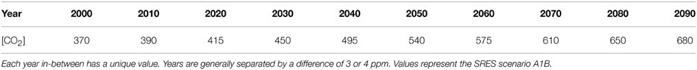
Table 2. Numerical values of [CO₂] concentrations in ppm used in this study in 10-year steps.

2.5. Statistics

To determine how the climatic input variables and [CO₂] affect biomass yields, a multivariate linear regression (MLR) model was used. This provided the ability to determine each input variable's significance as well as the strength and direction of its influence. The MLR model was applied for two distinct approaches.

Approach I, the results of which are displayed in Figure 2, uses 11 input values as independent variables for the MLR. These include 5 temperature and precipitation values respectively (annual, winter, spring, summer, fall), as well as atmospheric CO₂ concentration. This was done to incorporate all relevant variables within a single model to give an impression of how they influence the outcome in comparison to each other. The MLR was calculated in the following form (Faraway, 2002; Schönwiese, 2013):

$\begin{array}{cc}\begin{array}{l}Y={\beta }_0+{\beta }_1·C{O}_2+{\beta }_2·P_{Win}+{\beta }_3·P_{Spr}+{\beta }_4·P_{Sum}\hfill \\ +{\beta }_5·P_{Fal}+{\beta }_6·P_{Annual}+{\beta }_7·T_{Win}+{\beta }_8·T_{Spr}\hfill \\ +{\beta }_9·T_{Sum}+{\beta }_{10}·T_{Fal}+{\beta }_{11}·T_{Annual}+ϵ\hfill \end{array}& \left(1\right)\end{array}$

with Y as the effect variable; β₀ as the so-called Intercept or the general shift of the entire model along the y-axis; the coefficients β₁ through β₁₁ denoting how strong the change in their subsequent parameter would influence the outcome Y (in a fictional example β₁₁ = 150 would indicate that a rise in annual mean temperature would result in a rise in yields by 150 g∕m²); ϵ is commonly referred to as error term that represents variables omitted in the equation.

FIGURE 2

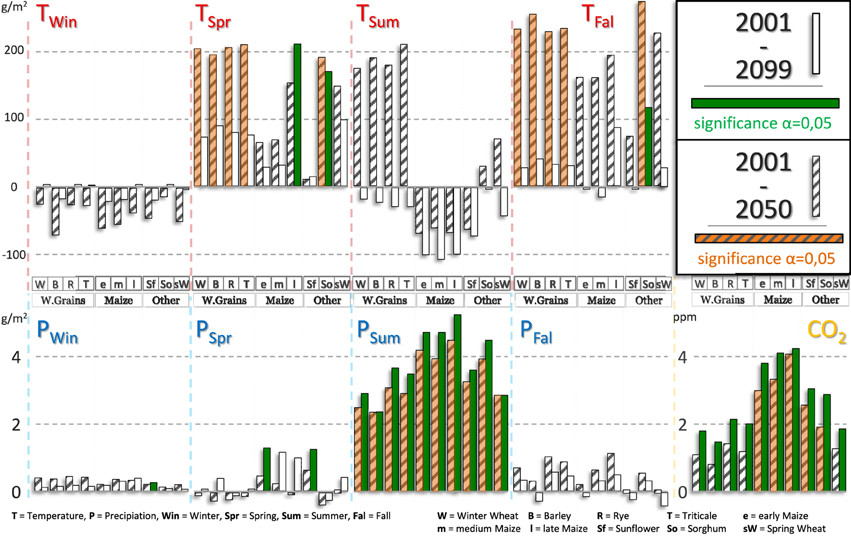
Figure 2. Results from the multivariate regression model. Mean values of 91,014 multivariate regression models for each of the time-spans 2001–2099 and 2001–2050. Bar heights indicate regression strength and direction. Bar color indicates significance. Values are given for each crop for four different precipitation and temperature periods as well as for [CO₂]. Example: A green value of +2 of P_sum means that if summer precipitation rises by 1 mm, yields would rise by 2 g/m² with α < 0.05 for the time 2001–2099.

Due to processing time limitations this equation was solved only for half of all available sites (about 40,000). This was done for two different periods, 2001–2050 and 2001–2099, to determine if the influence of single variables changes throughout the century. Using a t-test the significance of each variable during each period is determined. It is assumed that a variable is significant for α < 0.05. For each time period each site resulted in one p-Value derived from the t-test. The displayed results are the averages of all 40,000 sites.

Single-colored bars in Figure 2 always refer to period 2001–2099 while striped bars always refer to period 2001–2050. Colorless bars represent no significance and colored bars represent significance. For each independent variable there exist exactly 20 bars, representing the 10 crops in the 2 periods. Note that in Figure 2, the annual temperature and precipitation are not displayed, as they are never significant and of vastly different scale than the displayed seasonal variables.

Approach II was devised in order to verify the results from Approach I. This becomes necessary as auto-correlation is very likely to occur in Approach I, as at least temperature trends seem to be relatively equal across the five variables. However, auto-correlation in MLR models can lead to variables appearing as significant even if they are not or vice versa.

In principle, this second approach determines the best MLR model for each individual site by constructing every single possible MLR-equation using 11 independent variables. In total, there exist 2047 unique ways to construct an MLR-equation from 11 variables if their order is neglected (compare Figure 3). Each of these 2047 equations was calculated for a total of 3740 randomly distributed sites (resulting in 7,655,780 MLR model runs) due to computational efficiency. The MLR model quality, or how well a particular set of independent variables could explain the output yield, was determined by an F-test. Generally speaking, the larger the F-test value, the better one MLR model was suited to explain the yield output. The MLR model with the highest F-value was then logged for each site. Sites where several MLR models share equal F-values get the one MLR model assigned that uses the least number of input variables.

FIGURE 3

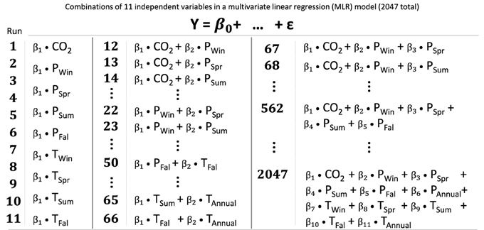
Figure 3. Schematic of how variables were sampled for the MLR models of Approach 2 in Section 2.5.

All statistics in this study have been calculated using MS Excel 2010 and Python (v 2.7) with the addition of SCIPY and NUMPY (Jones et al., 2001), Pandas (McKinney, 2010) and MATPLOTLIB (Hunter, 2007). For the calculation of the multivariate regression models R (v 2.15.2) and rpy2 (v 2.3.0) came to use as well.

3. Results

3.1. Climate Change in Niedersachsen

As displayed in Figure 4, the annual precipitation average will change only slightly over the course of the twenty-first century. Until 2070, the annual mean is reduced by less than 2%. Almost everywhere in NI the precipitation changes are below a rate of ±10%. In the period 2071–2100, the annual average decreases by 6%, with an extending area, decreases more than 10%.

FIGURE 4

Figure 4. Climate Change in Niedersachsen. Maps depict the mean change in temperature or precipitation respectively for the given time period. Changes are relative to 1971–2000. Temperature differences are in degree centigrade, precipitation differences in percent. The bars indicate the overall mean for Niedersachsen, with the bold bar indicating annual averages and the other bars for each season. The model used was Wettreg2010 with scenario A1B.

A greater divergence becomes apparent when precipitation values are not considered annually but rather by season. While spring and fall changes are pretty close to the annual changes (i.e., practically non-existent), winter and summer changes are drifting apart into opposite directions. This development can first be seen for the period 2041–2070, when winter precipitation increases by 8.2% as opposed to −13.2% in summer. Until the end of the century, this trend strengthens, especially for the decreases in summer. In 2071–2100, summer precipitation will on average be −25.2% below today's—with local outliers close to −50%. However, the increases in winter precipitation, on average +12.9% with outliers close to +40%, lack in necessary substance to compensate the severe summer losses in its entirety.

In contrast to precipitation changes, the temperature development is only directed into one direction: up. There are neither any time spans nor any regions in NI that will experience a stagnant or even declining temperature development until 2100. However, that does not implicate uniformity in development. Locally, the south-east will undergo the strongest development, the north-west the lowest, respectively. This pattern follows the increasing continentality as the north-west is more maritime influenced. Differences between both extremes amount to roughly 1°C.

By season, it's again the summer and even more so the winter months that heat up above average. For 2071–2100, the model results suggest increases of >4.5°C in winter and >4°C in summer. Spring and fall are always below average, with spring temperatures showing the least increases.

In short, the deviations from today's climate will increase with passing time, fostering a local development toward a more winter rain climate that features increasingly hot and dry summers and mild wet winters.

3.2. Yields Development: State Average

As becomes quickly evident from Figure 5 and Table 3, different [CO₂] levels have an obvious effect on the resulting crop yields throughout the twenty-first century. Again, results are given relative to 2001–2010.

FIGURE 5

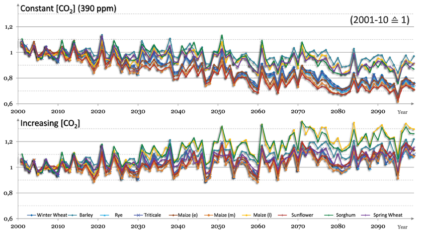
Figure 5. Biomass development with constant and changing [CO₂]. Top: biomass development throughout the 21st century if [CO₂] is hold constantly at 390 ppm-Below: Same modeling approach as above, only [CO₂] is changed for each year according to SRES scenario A1B.

TABLE 3

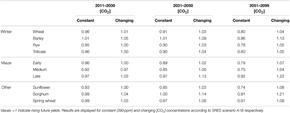
Table 3. Quotient of crop biomass of specified periods in relation to 2001–2010 (=1).

This effect will gain strength with passing time. In the near future (2011–2030), modeling with increasing [CO₂] will result in average yield increases of merely 1.3%, with a maximum of 5% for barley. If modeled with a constant level of 390 ppm, almost all crops show a decline in yields — on average −3.6% but as much as −8% for the medium maize variety. Only the yield of barley will still increase, though small at just 1%.

If the second half of the century is regarded, crop yields rise on average 9.7% with rising [CO₂]. The spread between the crops is, however, substantially larger than at the beginning of the century. Barley (13%), sorghum (21%) and the late maize variety (22%) benefit greatly, while winter wheat, rye, triticale and the late maize variety remain below 5% increases.

A constant [CO₂] now results in an average decline, over all 10 crops, of −16.4%. Only barley (−4%) can barely keep up with today's yields. The other winter grains (≤ − 20%) and especially the medium maize variety (−25%) and sunflower (−26%) would suffer dramatically under a future climate if a [CO₂] fertilization effect was to be neglected. These effects would be even worse if the last decade(s) would have been chosen for comparison instead of the entire century's half.

A constant [CO₂] leads, furthermore, to a more linear development. Assuming a linear trend, yields decline with an average R² = 0.60 (between barley 0.24 and the late maize variety 0.83) under constant [CO₂] but increase only with an average R² = 0.28 (between rye 0.08 and the late maize variety 0.64) when [CO₂] concentrations are adapted. Interestingly, the coefficient of variability (COV) per decade follows the same pattern for both model runs, ascending toward the middle of the century and descending afterwards, but the use of 390 ppm [CO₂] leads to a slightly higher variability. The decade with the highest variability for both runs, 2051–2060, has a COV of 7.0% when [CO₂] is elevated and 8.4% at 390 ppm. The differences in the other decades are generally around 0.5%. Relative to the decadic mean an elevated [CO₂], thus, has a dampening effect on outliers.

Figure 6 emphasizes on the yield differences of each crop between their two modeling approaches throughout the century. While barley and spring wheat are relatively robust toward the end of the century, with yield differences around 20%, sunflower and the medium maize variety surpass or come close to the 50% mark. To put it into other words, if the last decade of the century is considered, a [CO₂] concentration of roughly 1.8×390 ppm, as described by SRES-A1B, would lead to about 1.5× larger sunflower yields.

FIGURE 6

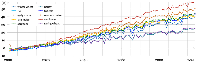
Figure 6. Biomass yield difference between constant and changing [CO₂]. A value of +20% would indicate that biomass yields are 20% higher when modeled using increasing [CO₂] instead of fixed 390 ppm.

As early as about 2020, sunflower clearly separates itself from the bulk of the other crops, which develop quite similar in a relatively narrow corridor with differences around 40% toward the century's end. Barley and spring wheat split from this bulk around the year 2040, medium and early maize around the year 2055.

3.3. Yields Development: Regional Differentiation

Yield differences are not solely found between different crops but also between regions, as can be seen in Figure 7. While those crops whose yield development is strongly influenced by a rise in [CO₂] (e.g., sunflower) or very weakly (e.g., barley and spring wheat) show a rather uniform regional development, the others do not necessarily. On average, the research area's east or north-east depends the most on rising [CO₂] for a positive yield development. The south has also a substantial number of areas where differences between both [CO₂] scenarios are above 60%.

FIGURE 7

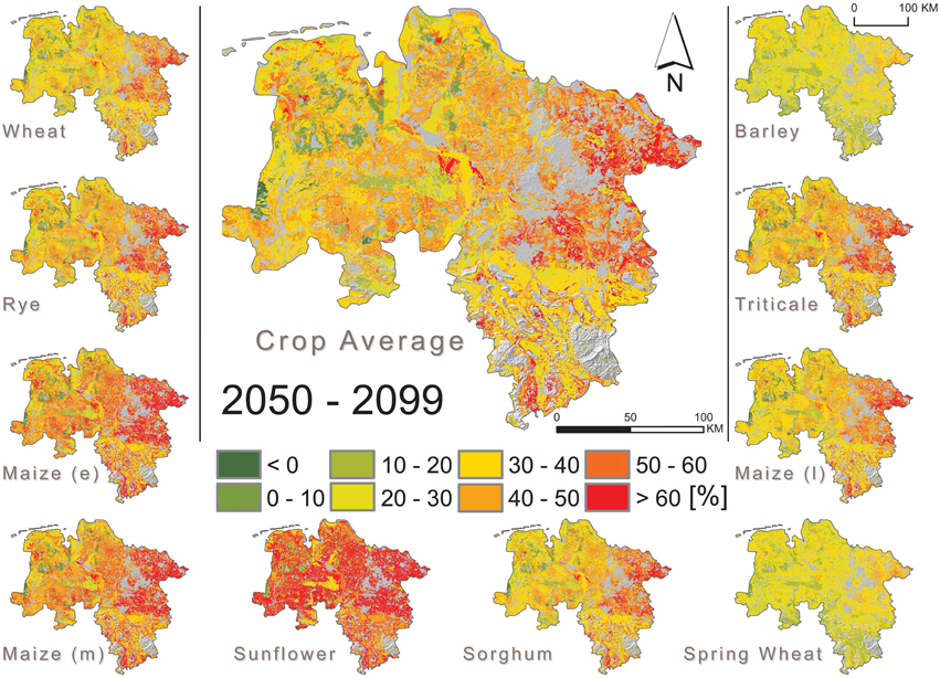
Figure 7. Spatial percentage variation between crop yields modeled with constant and changing [CO₂]. A value of +20% would indicate that biomass yields are 20% higher when modeled using increasing [CO₂] instead of fixed 390 ppm.

The least differences can be found to the west and north-west. However, only 2% of all sites have yield differences <10% anyway, while almost 10% of the sites have differences >60%.

A simple correlation between the mean modeling spread (Figure 6) and the respective soil's available water capacity (AWC) of all 91,014 sites results in a correlation coefficient of r = −0.66. Thus, the higher the AWC, or the more water a soil can store, the smaller is the difference between a modeling approach with constant or adapted [CO₂]. The strongest relation can be found in the south (official Region 8.2 Degener, 2013) with r = −0.91. Alternating good and bad soils do also show alternating large or small modeling differences. This is a clear indicator that the soil's ability to retain larger amounts of water will have a critical influence on crop yields. Interestingly though, the area with the weakest correlation of r = −0.52 is the one to the north-east (official Region 5.2 Degener, 2013). Soils in this region are generally of poor quality and precipitation is already quite low today. It seems that there are too few good soils that could make a difference or that the climatic changes will be so severe that even the better soils cannot fully absorb the negative impacts caused by reduced precipitation.

3.4. Statistical Analysis

The results from the MLR model consisting of 11 variables (Approach 1, see above) indicate that six of the independent variables (T_Win,T_Sum,T_Annual,P_Win,P_Fal,P_Annual) almost never show a significant relation with the resulting yields.

For the period 2001–2099, it is almost a sole matter of the two variables P_Sum and [CO₂] on the question how yields will develop. Only plants like the late maize variety or sorghum, which are in need of higher temperature sums than are currently present in the research area for a full development cycle, are additionally affected by a rise in temperatures and here especially in T_Spr.

If, however, only the first half of the century is regarded, the quantitative annual influence of P_Sum and [CO₂] is reduced. Even more, for winter grains and spring wheat, the [CO₂] influence is no longer significant, as the temperature development in the early century will be of greater importance. However, this rise in temperature becomes quickly detrimental to a healthy plant growth, as the quantitative influence is strongly reduced if the entire century is regarded and is possibly negative if only the second half would be regarded. This is especially true for summer temperatures. While they do not significantly influence yields (they would, however, for 0.05 < α < 0.10), their impact changes from strongly positive in the first half to slightly negative if the entire century is concerned for winter grains, sorghum and spring wheat. For maize and sunflower, summer temperatures have a negative impact regardless of the chosen period, though also not significant in the chosen MLR model.

These results hold true even if auto-correlation is ruled out by choosing the best multivariate model for each site (Approach 2, compare Figure 8). For 2001–2099, the best MLR model would solely contain both P_Sum and [CO₂] to describe the yield development across 76% of all sites and crops. Twelve percent would use a model only containing spring temperatures (T_Spr). This is mostly true for barley, as on more than 50% of all sites, it uses only spring temperatures as its optimal MLR model, while almost none of the other crops uses this scenario as the optimal one.

FIGURE 8

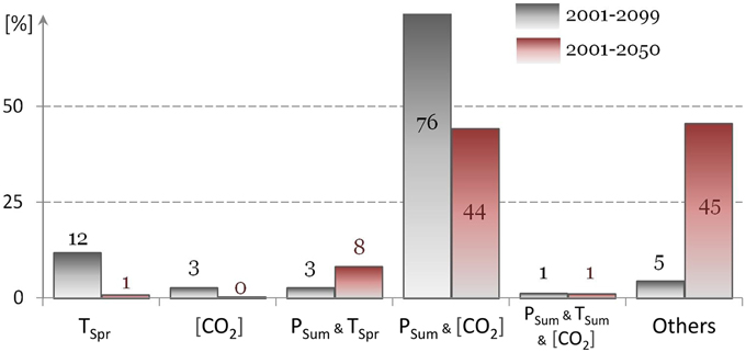
Figure 8. Percentage of optimal MLR models by model composition and time periods. The presented list of model combinations is not exhaustive.

For 2001–2050, only 44% of all sites and crops would use a model consisting of P_Sum and [CO₂]. The remaining models often consist of a combination of P_Sum and T_Spr; however, there is now a much larger number of different variable combinations than for 2001–2099. 45% of these best MLR models are thus classified as “Others” in Figure 8. These “Others” are now much more dependent on the respective crop. A large part of these other models for winter grains (excluding barley) as well as for early and medium maize uses only P_Sum as the optimal model. For the late maize variety and sorghum, now models only featuring T_Fal are showing up quite often.

4. Discussion

All of these results point into one direction. The basic climatic factors like precipitation and temperature will change in a way detrimental to the growth of crops. While increasing temperatures are beneficial at first to winter grains and spring wheat, they will increasingly inhibit an optimal development throughout the seasons. Maize is already today grown at near optimal temperatures, thus even small temperature change upwards, show negative effects on maize yields (Schlenker and Roberts, 2009). Even worse is the development of precipitation, especially during the summer months, the main growing season of most crops. Declines of about 25%, on average, are more than substantial and can potentially disrupt the known agricultural structure of NI. Only crops with a substantial part of their growth phase outside of the dry summer months, like barley before or late maize before and after, could defy the negative effects of climatic change without further external changes, at least to some degree.

This is supported by the results from the MLR models, as mostly two variables will have a major impact on future crop yields: summer precipitation (P_Sum) and [CO₂]. Both significantly and positively correlate with crop yields. As P_Sum is declining, this positive correlation will diminish yields, whereas rising [CO₂] levels will increase them. Both effects are stronger for the length of the entire century as compared to its first half. Drought stress and the ability to counter this stress are thus increasingly the defining factors for plant growth in the course of the twenty-first century.

The effects of reduced water availability can also be found in the regional pattern of larger soil areas within NI (Eckl and Raissi, 2009). Sites with yield differences above 60% between the scenario with constant and changing [CO₂] can mainly be found to the east and north-east, a region characterized by sandy soils and average precipitation of less than 700 mm annually. Even worse, those regions are among those with the strongest decline in summer precipitation with a reduction of 30–40% in the last decade (Degener, 2013). A similar connection can be found in the south. Here, very poor soils in the hills alternate with rather excellent soils in the quite fertile river valleys. The poorer sites almost exclusively differ >60% in yields in the second half of the century, whereas the good sites are about average for Niedersachsen. While the average summer precipitation is also reduced by about 30% in the south, the total amount of precipitation is substantially higher at the end of the century compared to parts farther east.

The effects of rising temperatures and declining precipitation might even be underestimated in this study as they were fed as monthly means into the crop model. The model then assumes that both variables are distributed evenly over all days of the month thus eliminating the impact of extreme events from the data. It is, however, expected that frequency and magnitude of such extreme events will increase in Germany and thus within NI (Beniston et al., 2007). Related to this, the model did not take into account the more sensitive growing stages of the plants where drought stress would have led to a disproportionately larger yield drop (Ehlers, 1996).

It is, therefore, quite conceivable for the yields to be reduced even lower than −17% on average in the second half of the century as depicted in this study. The more important becomes the one factor that counteracts this negative trend: the atmospheric CO₂ concentration. Not only is the described negative climatic effect balanced out, it is reversed by a rise in [CO₂] if it would follow the increases of the A1B scenario. A former yield reduction is now an increase of roughly 10%. However, this does not affect all crops similarly. In literature, it is often indicated that in C₃-species photosynthesis and dry matter production are generally stimulated positively by elevated [CO₂] levels while C₄-crops show little to none (Fleisher et al., 2011). While this will hold true on many occasions, it clearly does not within the scope of this study.

The one crop benefiting most from an elevated [CO₂] level is sunflower, a C₃-crop (Figure 6). The next two crops in line are, however, C₄-crops, early and medium maize variety. On the other hand, the two crops that benefit the least are C₃-crops, barley and spring wheat. Therefore, C₃-crops do not seem to necessarily benefit more from higher [CO₂] levels in general. As already described, elevated [CO₂] levels will increase the water use efficiency (WUE) in C₃- as well as in C₄-plants. This water saving effect seems to be here of greater importance than an elevated photosynthesis rate. That this magnitude is conceivable has been argued before (Taube and Herrmann, 2009) with an example of Grasslands profiting from a rise in [CO₂] even under considerable summer drought stress. Under some circumstances, the water saving aspect is thus much more important than the direct fertilization effect (Morgan et al., 2004) and might well be for locations other than Niedersachsen.

An example to further support this point are the three maize varieties. While the physiological processes are quite similar in the early, medium and late variety, and are also treated almost equally within the model, their absolute yield differences are mostly subject to different temperature sums and thus the length and time of their growing seasons. As Table 3 shows, the differences in the relative yield development are quite substantial and the factor that could account for such difference must be connected to the growing season. While the late variety will at first also benefit from rising temperatures, today's sums are not sufficient to reach full maturity; its exceptional yield gains in relation to the other two varieties needs more explanation. The idea is thus, supported by the results from the multivariate regression analysis, that summer precipitation again plays a major role to describe the yield development. More precisely, the more time a plant spends during the drier summer months, in relation to its entire growing season, the more negative its yield development will be. The late variety may experience sufficient water input during the spring and fall months, the early variety in spring. The medium variety may also use the spring months, where precipitation is expected to remain more or less constant but would grow longer during the drier summer season. In accordance to similar studies (Southworth et al., 2000), it could thus be concluded that a plant's ability to evade the drier summer months, by shorter or longer growing seasons, will be crucial to at least maintain current yield levels. This will go hand in hand with an adaption of sowing dates that was, however, not applied in this study, though initial testing would suggest that especially, medium and early variety would benefit from earlier sowing dates.

The same pattern of the maize varieties can be found for the winter grains. The one grain that is harvested before all others, barley, will have the least negative effects of reduced summer precipitation, as it again spends a relatively short amount of time growing in the drier summer. Sunflower, a crop with huge water demand (Ehlers, 1996), will benefit disproportionately from an increased WUE when water becomes more scarce. Therefore, it is no surprise to see the largest discrepancies in yields for sunflower when modeled with or without rising [CO₂]. Sorghum, adapted to hot and dry climates, will also show substantial yield increases simply due to expected warming in Germany but can also cope with the drier summer months due to its adapted physiology. In this regard, it is comparable to the late maize variety.

That [CO₂] is of such importance for future plant development now raises two concerns. (1) is the expected influence of [CO₂] as strong as depicted by the crop model and (2) will [CO₂] levels change as assumed under the A1B IPCC scenario?

(1) As mentioned before, there is an active discussion about this question (Long et al., 2006; Fleisher et al., 2011; Kimball, 2011; McGrath and Lobell, 2013). Even more, there is rather little knowledge on the interaction of [CO₂], temperature, water and nutrient availability and other site characteristics. However, the overall notion tends toward yield results under elevated [CO₂] that are below those estimated in today's crop models. Nevertheless, this is still an open question and it may very well be that chamber experiments with elevated [CO₂] overestimate yields while open atmosphere experiments underestimate them (Kimball, 2011). While it is hard to quantify the difference, especially given the heterogeneous structure of the research area, it could be assumed that yields achieved under adapted [CO₂] are still overestimated in this study. As at least some effect is expected though, it seems also unrealistic to assume that the model runs using 390 ppm are closer to the truth and the real yield changes might possibly lie somewhere in-between.

(2) [CO₂] levels will probably not change exactly as depicted in any of the SRES scenarios. The question remains how certain we are today that the general development will be as described, especially considering that these scenarios were devised one and a half decades ago. Figure 9 presents a comparison of the more recent RCP scenarios with the SRES-A1B scenario used in this study. It should, however, be noted that in contrast to the SRES scenarios, the RCP [CO₂] pathways are not fixed but are rather probable courses under the assumed change in radiative forcing (Moss et al., 2010). The presented RCP [CO₂] concentrations can thus vary between studies. Except for the worst-case scenario, RCP 8.5, all other scenarios have lower [CO₂] concentrations throughout most of the twenty-first century than A1B. However, even RCP 8.5 would be slightly lower than A1B around the 2040s in this data-set. Therefore, [CO₂] concentrations might be overestimated in this study. A decreased fertilization effect and WUE would be the case.

FIGURE 9

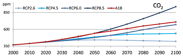
Figure 9. Possible RCP [CO₂] pathways compared to the SRES A1B scenario. RCP Data was taken from the RCP-Database (Kolp and Riahi, 2013).

In how far both assumptions will become an issue in reality must be a future discussion as today's data is not sufficient to further clarify this subject.

Related to these uncertainties, it should be noted that apart from the choice of scenario, the global circulation model (GCM) and the related downscaling approach introduce uncertainties of their own. In short, this comprises four aspects: initial conditions, boundary conditions, parametrization as well as structural insecurities (Tebaldi and Knutti, 2007; Knutti et al., 2010). These inevitably lead to projections of the climate that will not match the future in detail. However, as Flato et al. (2013, p.825) point out in the last IPCC report “(…) climate models are based, to a large extent, on verifiable physical principles and are able to reproduce many important aspects of past response to external forcing. In this way, they provide a scientifically sound preview of the climate response to different scenarios of anthropogenic forcing.”

Similarly, the crop model introduces uncertainties of its own. There are two ways this article addresses these concerns. One is the comparison of measured field data and modeled data for the years 2006–2010. With error margins generally below 10%, the model is able to represent the reality reasonably well. It might be argued that at least for the early twenty-first century this lies within the model's error range. However, this study focuses on changes in future yields, whereas both today's and future yields are calculated within the model. Using this delta change approach, there is no emphasis on absolute future yields (e.g., in g/m²); thus, the distortion of results is at least reduced as the model's internal bias should be the same for today and for the future. The other way is to compare the output of similar simulations. As mentioned in the introduction, the available results for winter wheat are quite similar to those presented in this study. This is true for the general direction of the yield trends (downward without elevated [CO₂], upward when elevated) as well as for the magnitude of these trends.

The results presented in this study are in accordance with these observations and the uncertainties of both climate and crop model are acknowledged when discussing the study's outcome. Therefore, the presented results should be considered as projections rather than predictions.

Furthermore, there are several other aspects to consider that are, however, not discussed in depth within this study. These include an altered metabolism of plants under changed [CO₂] concentrations, with all possible kinds of implications on plant growth, protein content, leaf morphology, etc. (Ziska, 2011). Another is the interaction with tropospheric ozone that is hazardous to plant growth. The idea is that even when tropospheric O₃ concentrations rise, the effect might be reduced when closed stomata due to elevated [CO₂] prevent the ozone from entering the plants (Fuhrer, 2009).

On the other hand, it could be questioned if declining summer precipitation will really have such a destructive effect, even if [CO₂] effects are neglected, as irrigation is a viable option in northern Germany. Groundwater management to balance the summer water losses with increased winter precipitation would be one key to this approach (Müller et al., 2012).

Conflict of Interest Statement

The author declares that the research was conducted in the absence of any commercial or financial relationships that could be construed as a potential conflict of interest.

Acknowledgments

We acknowledge support by the German Research Foundation and the Open Access Publication Funds of the Göttingen University.

Abbreviations

[CO₂], atmospheric carbon dioxide; AWC, available water capacity; COV, coefficient of variability (standard deviation divided by mean value); GCM, Global Climate Model; NI, Niedersachsen, state in Germany; MLR, multivariate linear regression; P_x, precipitation sums of x (win, winter, spr, spring, sum, summer, fal, fall); RMSE, Root Mean Square Error; T_x, temperature means of x (win, winter, spr, spring, sum, summer, fal, fall); WUE, water-use-efficiency.

References

Bauböck, R. (2013). GIS-gestützte Modellierung und Analyse von Agrar- Biomassepotentialen in Niedersachsen – Einführung in das Pflanzenmodell BioSTAR. PhD thesis, Georg-August-Universität, Göttingen.

Bauböck, R. (2014). Simulating the yields of bioenergy and food crops with the crop modeling software BioSTAR: the carbon-based growth engine and the BioSTAR ET0 method. Environ. Sci. Eur. 26, 1–9. doi: 10.1186/2190-4715-26-1

CrossRef Full Text

Beniston, M., Stephenson, D. B., Christensen, O. B., Ferro, C. A. T., Frei, C., Goyette, S., et al. (2007). Future extreme events in European climate: an exploration of regional climate model projections. Clim. Change 81, 71–95. doi: 10.1007/s10584-006-9226-z

CrossRef Full Text | Google Scholar

Boess, J., Gehrt, E., Müller, U., Ostmann, U., Sbresny, J., and Steininger, A. (2004). Erläuterungsheft zur digitalen nutzungsdifferenzierten Bodenkundlichen Übersichtskarte 1:50.000 (BÜK50n) von Niedersachsen, Vol. 3 of Arbeitshefte Boden. Hannover: LBEG (State Authority for Mining, Energy and Geology).

Chmielewski, F.-M. (2007). “Folgen des klimawandels für land- und forstwirtschaft,” in Der Klimawandel, ed W. Endlicher (Potsdam: Potsdam-Inst. für Klimafolgenforschung), 75–85.

Degener, J. (2013). Auswirkungen des regionalen Klimawandels auf die Entwicklung der Biomasseerträge ausgewählter landwirtschaftlicher Nutzpflanzen in Niedersachsen. PhD thesis, University of Goettingen, Göttingen.

DeStatis. (2013). Statistical Yearbook of Germany 2013, 1 Edn. Wiesbaden: Statistisches Bundesamt.

Drachenfels, O. (2010). Überarbeitung der naturräumlichen regionen niedersachsens. Inf. Naturschutz Niedersachsen 30, 249–252.

DWD. (2014). Website of the German Weather Service. Offenbach: Deutscher Wetterdienst.

Eckl, H., and Raissi, F. (2009). Leitfaden für hydrologische und bodenkundliche Fachgutachten bei Wasserrechtsverfahren in Niedersachsen. Hannover: Landesamt für Bergbau, Energie und Geologie (LBEG).

Ehleringer, J. R., and Cerling, T. E. (2002). “The earth system: biological and ecological dimensions of global environmental change,” in Encyclopedia of Global Environmental Change, eds H. A. Mooney and J. G. Canadell (Chichester: John Wiley & Sons, Ltd.), 186–190.

Ehlers, W. (1996). Wasser in Boden und Pflanze: Dynamik des Wasserhaushalts als Grundlage von Pflanzenwachstum und Ertrag. Stuttgart: Ulmer (Eugen).

Google Scholar

Enke, W., Deutschlander, T., Schneider, F., and Kuchler, W. (2005). Results of five regional climate studies applying a weather pattern based downscaling method to ECHAM4 climate simulation. Meteorol. Z. 14, 247–257. doi: 10.1127/0941-2948/2005/0028

CrossRef Full Text | Google Scholar

Enke, W., and Spekat, A. (1997). Downscaling climate model outputs into local and regional weather elements by classification and regression. Clim. Res. 8, 195–207. doi: 10.3354/cr008195

CrossRef Full Text | Google Scholar

Faraway, J. (2002). Practical Regression and Anova using R. Available online at: www.cran.r-project.org/doc/contrib/Faraway-PRA.pdf.

Flato, G., Marotzke, J., Abiodun, B., Braconnot, P., Chou, S. C., Collins, W., et al. (2013). “Evaluation of climate models,” in Climate Change 2013: The Physical Science Basis. Contribution of Working Group I to the Fifth Assessment Report of the Intergovernmental Panel on Climate Change, eds T. F. Stocker, D. Qin, G.-K. Plattner, M. Tignor, S. K. Allen, J. Boschung, A. Nauels, Y. Xia, V. Bex, and P. M. Midgley (Cambridge; New York: Cambridge University Press), 741–866. doi: 10.1017/CBO9781107415324.020

CrossRef Full Text

Fleisher, D., Timlin, D., Reddy, K., Reddy, V., Yang, Y., and Kim, S. (2011). “Effects of CO2 and temperature on crops: lessons from SPAR growth chambers,” in Handbook of Climate Change and Agroecosystems, Volume 1 of ICP Series on Climate Change Impacts, Adaptation, and Mitigation, eds D. Hillel and C. Rosenzweig (London: Imperial College Press), 55–86.

Fuhrer, J. (2009). Ozone risk for crops and pastures in present and future climates. Naturwissenschaften 96, 173–194. doi: 10.1007/s00114-008-0468-7

PubMed Abstract | CrossRef Full Text | Google Scholar

Gaastra, P. (1959). Photosynthesis of Crop Plants as Influenced by Light, Carbon Dioxide, Temperature, and Stomatal Diffusion Resistance. Wageningen, NL: H. Veenman & Zonen N.V.

Google Scholar

Heunisch, C., Caspers, G., Elbracht, J., Langer, A., Röhling, H.-G., Schwarz, C., et al. (2007). Erdgeschichte von Niedersachsen: Geologie und Landschaftsentwicklung. Hannover: Landesamt für Bergbau, Energie und Geologie (LBEG) Geoberichte (6).

Hoffmann, F. (1995). FAGUS, a model for growth and development of beech. Ecol. Model. 83, 327–348. doi: 10.1016/0304-3800(94)00101-8

CrossRef Full Text | Google Scholar

Högy, P., and Fangmeier, A. (2008). Effects of elevated atmospheric CO2 on grain quality of wheat. J. Cereal Sci. 48, 580–591. doi: 10.1016/j.jcs.2008.01.006

CrossRef Full Text | Google Scholar

Huang, S., Krysanova, V., and Hattermann, F. (2012). “Impacts of climate change on water availability and crop yield in germany,” in Conference: International Environmental Modelling and Software Society (iEMSs) (Leipzig).

Google Scholar

Hunter, J. D. (2007). Matplotlib: A 2D graphics environment. Comput. Sci. Eng. 9, 90–95. doi: 10.1109/MCSE.2007.55

CrossRef Full Text | Google Scholar

Jones, E., Oliphant, E., Peterson, P., et al. (2001). SciPy: Open Source Scientific Tools for Python. Available online at: http://www.scipy.org/

Kersebaum, K., and Nendel, C. (2014). Site-specific impacts of climate change on wheat production across regions of Germany using different CO2 response functions. Eur. J. Agron. 52, 22–32. doi: 10.1016/j.eja.2013.04.005

CrossRef Full Text | Google Scholar

Kimball, B. (2011). “Lessons from FACE: CO2 effects and interactions with water, nitrogen and temperature,” in Handbook of Climate Change and Agroecosystems, Vol. 1 of ICP Series on Climate Change Impacts, Adaptation, and Mitigation, eds D. Hillel and C. Rosenzweig (London: Imperial College Press), 87–108.

Kimball, B., Kobayashi, K., and Bindi, M. (2002). “Responses of agricultural crops to free-air CO2 enrichment,” in Advances in Agronomy, Vol. 77, ed D. L. Sparks (Newark, DE: Elsevier), 293–368. doi: 10.1016/s0065-2113(02)77017-x

CrossRef Full Text

Knutti, R., Furrer, R., Tebaldi, C., Cermak, J., and Meehl, G. A. (2010). Challenges in combining projections from multiple climate models. J. Climate 23, 2739–2758. doi: 10.1175/2009JCLI3361.1

PubMed Abstract | CrossRef Full Text | Google Scholar

Kolp, P., and Riahi, K. (2013). RCP Web-Database: Version 2.0.5.

Kreienkamp, F., Spekat, A., and Enke, W. (2010). Weiterentwicklung von WETTREG bezüglich neuartiger Wetterlagen. Potsdam: Climate & Environment Consulting Potsdam GmbH.

Google Scholar

Lambers, H., Pons, T. L., and Chapin, F. S. (2008). Plant Physiological Ecology. 2nd Edn. New York, NY:Springer Verlag. doi: 10.1007/978-0-387-78341-3

CrossRef Full Text

Long, S. P., Ainsworth, E. A., Leakey, A. D. B., Nösberger, J., and Ort, D. R. (2006). Food for thought: lower-than-expected crop yield stimulation with rising CO2 concentrations. Science 312, 1918–1921. doi: 10.1126/science.1114722

PubMed Abstract | CrossRef Full Text | Google Scholar

LSN. (2014). Statistical Data of the Statistical Office of Lower Saxony. Hannover: Landesamt für Statistik Niedersachsen (LSN).

McGrath, J. M., and Lobell, D. B. (2013). Regional disparities in the CO 2 fertilization effect and implications for crop yields. Environ. Res. Lett. 8:014054. doi: 10.1088/1748-9326/8/1/014054

CrossRef Full Text | Google Scholar

McKinney, W. (2010). “Data structures for statistical computing in Python,” in Proceedings of the 9th Python in Science Conference, eds S. van der Walt and J. Millman, 51–56.

Google Scholar

Morgan, J. A., Pataki, D. E., Körner, C., Clark, H., Del Grosso, S. J., Grünzweig, J. M., et al. (2004). Water relations in grassland and desert ecosystems exposed to elevated atmospheric CO2. Oecologia 140, 11–25. doi: 10.1007/s00442-004-1550-2

PubMed Abstract | CrossRef Full Text | Google Scholar

Moss, R. H., Edmonds, J. A., Hibbard, K. A., Manning, M. R., Rose, S. K., van Vuuren, D. P., et al. (2010). The next generation of scenarios for climate change research and assessment. Nature 463, 747–756. doi: 10.1038/nature08823

PubMed Abstract | CrossRef Full Text | Google Scholar

Müller, U., Engel, N., Heidt, L., Schäfer, W., Kunkel, R., Wendland, F., et al. (2012). Klimawandel und Bodenwasserhaushalt. Hannover: Landesamt für Bergbau, Energie und Geologie (LBEG).

Nakicenovic, N., Alcamo, J., Davis, G., Vries, B. d., Fenhann, J., Gaffin, S., et al. (2000). Special Report on Emissions Scenarios : a special report of Working Group III of the Intergovernmental Panel on Climate Change. New York, NY: Cambridge University Press.

Nendel, C., Kersebaum, K., Mirschel, W., Manderscheid, R., Weigel, H.-J., and Wenkel, K.-O. (2009). Testing different CO2 response algorithms against a FACE crop rotation experiment. NJAS - Wageningen J. Life Sci. 57, 17–25. doi: 10.1016/j.njas.2009.07.005

CrossRef Full Text | Google Scholar

NMUEK. (2012). Empfehlung für eine niedersächsische Klimaanpassungsstrategie. Hannover: Niedersächsisches Ministerium für Umwelt, Energie und Klimaschutz.

Roeckner, E. (2009). ENSEMBLES STREAM2 ECHAM5C-MPI-OM SRA1B run1: World Data Center for Climate: CERA-DB ENSEMBLES2_MPEH5C_SRA1B_1_MM. Hamburg: World Data Center for Climate, DKRZ.

Rosenthal, D., and Tomeo, N. (2013). Climate, crops and lacking data underlie regional disparities in the CO2 fertilization effect. Environ. Res. Lett. 8:031001. doi: 10.1088/1748-9326/8/3/031001

CrossRef Full Text | Google Scholar

Schlenker, W., and Roberts, M. J. (2009). Nonlinear temperature effects indicate severe damages to U.S. crop yields under climate change. Proc. Natl. Acad. Sci. U.S.A. 106, 15594–15598. doi: 10.1073/pnas.0906865106

PubMed Abstract | CrossRef Full Text | Google Scholar

Schönwiese, C. (2013). Praktische Statistik fr Meteorologen und Geowissenschaftler. Stuttgart: Borntraeger.

Google Scholar

Seedorf, H. H., and Meyer, H.-H. (1992). Historische Grundlagen und naturräumliche Ausstattung. Wachholtz: Neumünster.

Soussana, J.-F., Graux, A.-I., and Tubiello, F. (2010). Improving the use of modelling for projections of climate change impacts on crops and pastures. J. Exp. Bot. 61, 2217–2228. doi: 10.1093/jxb/erq100

PubMed Abstract | CrossRef Full Text | Google Scholar

Southworth, J., Randolph, J., Habeck, M., Doering, O., Pfeifer, R., Rao, D., et al. (2000). Consequences of future climate change and changing climate variability on maize yields in the midwestern United States. Agri. Ecosyst. Environ. 82, 139–158. doi: 10.1016/S0167-8809(00)00223-1

CrossRef Full Text | Google Scholar

Steffen, W., and Canadell, P. (2005). Carbon Dioxide Fertilisation and Climate Change Policy. Canberra: Department of the Environment and Heritage, Australian Greenhouse Office.

Taube, F., and Herrmann, A. (2009). “Relative benefit of maize and grass under conditions of climatic change,” in Optimierung des Futterwertes von Mais und Maisprodukten, volume 331 of Landbauforschung / Sonderheft, ed F. J. Schwarz (Braunschweig: VTI), 115–126.

Tausz, M., Tausz-Posch, S., Norton, R., Fitzgerald, G., Nicolas, M., and Seneweera, S. (2013). Understanding crop physiology to select breeding targets and improve crop management under increasing atmospheric CO2 concentrations. Environ. Exp. Bot. 88, 71–80. doi: 10.1016/j.envexpbot.2011.12.005

CrossRef Full Text | Google Scholar

Tebaldi, C., and Knutti, R. (2007). The use of the multi-model ensemble in probabilistic climate projections. Philos. Trans. R. Soc. A Math. Phys. Eng. Sci. 365, 2053–2075. doi: 10.1098/rsta.2007.2076

PubMed Abstract | CrossRef Full Text | Google Scholar

Vanuytrecht, E., Raes, D., and Willems, P. (2011). Considering sink strength to model crop production under elevated atmospheric CO2. Agri. Forest Meteorol. 151, 1753–1762. doi: 10.1016/j.agrformet.2011.07.011

CrossRef Full Text | Google Scholar

Wang, L., Feng, Z., and Schjoerring, J. (2013). Effects of elevated atmospheric CO2 on physiology and yield of wheat (Triticum aestivum L.): a meta-analytic test of current hypotheses. Agri. Ecosyst. Environ. 178, 57–63. doi: 10.1016/j.agee.2013.06.013

CrossRef Full Text | Google Scholar

Weigel, H., and Manderscheid, R. (2012). Crop growth responses to free air CO2 enrichment and nitrogen fertilization: Rotating barley, ryegrass, sugar beet and wheat. Eur. J. Agron. 43, 97–107. doi: 10.1016/j.eja.2012.05.011

CrossRef Full Text | Google Scholar

Ziska, L., and Bunce, J. (2007). Predicting the impact of changing CO2 on crop yields: some thoughts on food. New Phytol. 175, 607–617. doi: 10.1111/j.1469-8137.2007.02180.x

PubMed Abstract | CrossRef Full Text | Google Scholar

Ziska, L. H. (2011). “Global climate change and carbon dioxide: assessingWeed biology and management,” in Handbook of Climate Change and Agroecosystems, Vol. 1 of ICP Series on Climate Change Impacts, Adaptation, and Mitigation, eds D. Hillel and C. Rosenzweig (London: Imperial College Press), 191–208.