The potential of satellite-observed crop phenology to enhance yield gap assessments in smallholder landscapes

Introduction

Currently, 805 million people on planet Earth are undernourished (FAO et al., 2014); with the majority of this food insecure population in developing countries, particularly, Sub-Saharan Africa and South Asia, where the rates of reduction in undernourishment are also slowest. Under the current food system a substantial proportion of the world's population is food insecure. Worryingly, projected increases in population and diets will require significant increases in food production (Tilman et al., 2011). This is problematic on numerous fronts; firstly, current trends in crop yield growth will fall short of meeting future demand (Ray et al., 2013); secondly, there is little room for expansion of croplands (Foley et al., 2011; Smith, 2013); thirdly, it highlights the complex interplay of socio-economic, political, cultural, and environmental factors that inhibit access to safe, sufficient, and nutritious food for sizeable vulnerable populations (Enfors, 2013; Pritchard et al., 2013; FAO et al., 2014). Expanding croplands is not an option for increasing crop production given environmental and developmental concerns (Rockström et al., 2009; Foley et al., 2011; Smith, 2013; Godfray and Garnett, 2014). Therefore, to address current and future food insecurity requires adjusting modes of access or demand for food, or increasing production on existing croplands.

A large proportion of the current level of undernourishment is borne by smallholder farmers in developing countries, particularly in Sub-Saharan Africa and South Asia (FAO et al., 2012; HLPE, 2013). Defining smallholder farmers is complex (HLPE, 2013), and different aspects of smallholding, such as size of land holding, asset levels, productivity of land or market engagement all influence a smallholder household's capacity to access food (Sen, 1981; Enfors, 2013; HLPE, 2013; Tittonell and Giller, 2013; Rammohan and Pritchard, 2014). The croplands in Sub-Saharan Africa and South Asia have the largest share devoted to producing crops for human consumption (Foley et al., 2011) whilst also suffering from the largest yield gaps (Mueller et al., 2012). Broadly put, yield gaps are the difference in crop yield between what is realized by farmers and what is potentially attainable in a given context (Tittonell and Giller, 2013; Van Ittersum et al., 2013). Different approaches have been utilized to measure and define yield gaps for specific contexts (Lobell et al., 2009; Licker et al., 2010). This suggests that closing yield gaps in smallholder landscapes can contribute toward the multiple goals of reducing food insecurity, increasing levels of crop production without negative environmental side-effects (Foley et al., 2011), catching up with projected demand (Ray et al., 2013), and improving the livelihoods of smallholders and their capacity to access food (Enfors, 2013; Tittonell and Giller, 2013; Dzanku et al., 2015).

Using data from household surveys across Sub-Saharan Africa, Dzanku et al. (2015) highlighted the elasticity between yield gaps and rural poverty, indicating that as yield gaps close the associated poverty also reduces. The concept of closing yield gaps in smallholder settings to enhance food security and poverty alleviation outcomes fits with the theory of poverty traps and development resilience (Barrett and Constas, 2014). The literature on poverty traps theorizes that certain thresholds in asset holdings exist which if exceeded lead to asset accumulation, higher returns (e.g., income, crop yield) and graduation to more desirable welfare levels (Carter and Barrett, 2006; Sabates-Wheeler and Devereux, 2011). In the context of yield gaps in smallholder croplands this theory suggests that if smallholders' assets (e.g., land, agricultural machinery, financial capital to purchase fertilizers and seeds, knowledge resources) are increased then they will receive higher returns from these assets, directly in the form of crop yield and indirectly through sales in markets. Through increased outputs, either through crop yield or incomes, smallholders will experience reduced levels of poverty and food insecurity enhancing their ability to access food via own-production or trade-based entitlements (Sen, 1981).

Closing yield gaps among smallholder croplands holds significant potential for poverty alleviation and food security (Dzanku et al., 2015). However, the context-specific nature of smallholder environments means that large amounts of data on the location, the magnitude, and the causation of yield gaps are required to effectively target responses. In other words, for such data to be utilizable in a policy-making sense, where the units of policy-making are much broader (e.g., region, country, global) than the scale at which yield gaps afflict the poorest and food insecure (e.g., plot-to-plot in smallholder settings) they must cover large extents without sacrificing local detail. These data requirements resonate with the characteristics provided by satellite sensor-derived remote sensing.

The data records accumulated through the Advanced Very High Resolution Radiometer (AVHRR), SPOT-VEGETATION (SPOT-VGT), Moderate Resolution Imaging Spectroradiometer (MODIS), and Medium Resolution Imaging Spectrometer (MERIS) have generated time-series of remote sensing imagery that enable monitoring of the intra-annual, and inter-annual, dynamics of vegetation growth. Vegetation growth dynamics is usually discerned through repeat satellite sensor observations of a location throughout the course of a growing season. From such observations, the vegetative signal is typically captured through various mathematical combinations of spectral reflectance in the red and near infrared (NIR) spectral bands into vegetation indices (VIs), such as the Normalized Difference Vegetation Index (NDVI) and the Enhanced Vegetation Index (EVI; Huete et al., 2002; Pettorelli et al., 2005), or through computation of biophysical variables, such as fraction of absorbed photosynthetically active radiation (fAPAR) or leaf area index (LAI; Duveiller et al., 2011; Meroni et al., 2014). Repeat satellite sensor observations of the land surface can reveal vast amounts of information about the dynamics of vegetation growth; this in turn can be used to estimate several phenological variables including the timing and length of seasons, and peak growing season (Pettorelli et al., 2005; Dash et al., 2010; Vrieling et al., 2011, 2013; Harris et al., 2014). Phenology refers to the timing recurring biological events (Brown and de Beurs, 2008).

Decades of research have shown spectral reflectance, and derived VIs, to be correlated with several biophysical variables including vegetation greenness, photosynthetic activity, canopy structure, biomass, and productivity (Tucker, 1979; Pinter et al., 1981; Huete et al., 2002; Pettorelli et al., 2005). It is this characteristic, and often via computing VIs, that makes remote sensing attractive for monitoring spatio-temporal patterns in vegetation growth and observing phenological transitions. However, given their prominence in remote sensing of vegetation it is important to note that different VIs have varying strengths and weaknesses with regards to monitoring vegetation; for example, the NDVI is chlorophyll sensitive whilst the EVI is more sensitive to canopy structure and related variables, such as LAI (Huete et al., 2002). The NDVI has been critiqued for scaling problems, the non-linear relationship with vegetation fraction within pixels (Lobell and Asner, 2004; Jiang et al., 2006), saturation at high biomass levels, and sensitivity to canopy background variation (Huete et al., 2002). Gitelson (2004) demonstrated how the NDVI did not capture variability in fraction of vegetation cover above 60% or LAI greater than two and posited the wide dynamic range vegetation index (WDRVI) as being more suitable. These differences in VIs will have subsequent impacts upon abilities to monitor vegetation, to estimate biophysical variables and observe phenological transitions.

Reflecting the value of phenological information to studies of vegetation growth and productivity (and a range of other fields) there are several “pre-processed” remote sensing data products available to facilitate observations of vegetation phenology. These include the Global Inventory Modeling and Mapping Studies (GIMMS) dataset produced using bi-monthly composites of AVHRR NDVI data at an ~8 km spatial resolution from 1981 to 2011 (see http://www.mdpi.com/journal/remotesensing/special_issues/monitoring_global for a special issue of Remote Sensing introducing the new GIMMS NDVI 3 g dataset). Several VI products are derived from MODIS data at a range of temporal and spatial resolutions (https://lpdaac.usgs.gov/products/modis_products_table); for example, the MOD09A1 product enables computation of NDVI and EVI at a 500 m spatial resolution in 8 day composites. Specific VI (e.g., MOD13A1) and vegetation phenology (e.g., MCD12Q2; Ganguly et al., 2010) products are also available from MODIS data. The MCD12Q2 product provides estimates of the date of various phenological transitions including onset of greenness, onset of maximum greenness, onset of decrease in greenness and minimum greenness along with associated EVI-values (Ganguly et al., 2010). Other coarse to medium resolution sensors which enable monitoring of land surface (and vegetation) phenology include SPOT-VGT and MERIS (see http://www.spot-vegetation.com/ and https://earth.esa.int/web/guest/missions/esa-operational-eo-missions/envisat/instruments/meris). Finer spatial resolution optical products are available from the Landsat Thematic Mapper (TM), Enhanced Thematic Mapper (ETM+), and Operational Land Imager (OLI) sensors carried on a succession of satellites with a 30 m spatial resolution (see http://landsat.usgs.gov/ for a review of the Landsat project). Other similar products exist, such as the imagery from the Linear Imaging Self Scanning (LISS) III sensor with a 23.5 m spatial resolution (see https://earth.esa.int/web/guest/data-access/browse-data-products/-/article/liss-iii-data-products-1660) and a range of other sensors with sub-10 m spatial resolutions (for example, Worldview, IKONOS, GeoEye). However, challenges persist with monitoring vegetation growth and dynamics with finer spatial resolution data due to infrequent revisit periods, obtaining sequences of cloud free images, and access to data.

Here, the capacity to monitor temporal profiles of vegetation growth via optical remote sensing, and estimate associated phenological variables, over smallholder croplands to enhance yield gap analysis is reviewed. Thus, there is a specific focus on monitoring crop growth and estimating crop phenological transitions. To ensure clarity in use of terms crop phenology when referred to at the plant scale refers to specific development stages crops go through (e.g., emergence, heading, anthesis), whereas remote sensing observations refer to less specific metrics (e.g., start-of-season, green up, peak growing season, end-of-season, onset-of-senescence); crop growth and crop growth dynamics refer to the green up and senescence cycles displayed by crops as they pass through phenological stages. It is worth mentioning that a range of sensors can reveal information on crop growth and phenology (e.g., radar, Shao et al., 2001; Li et al., 2003); however, this review is restricted to optical, satellite sensors. This focus on optical remote sensing is justified at the current moment; “long”-term records of optical imagery monitoring intra- and inter-annual dynamics in croplands, such as GIMMS AVHRR, SPOT-VGT and MODIS, have been accumulated permitting a large body of research to be conducted. Furthermore, we are about to enter a new phase of optical remote sensing with the recent launch of Landsat-8 and the imminent launches of Sentinel-2 and Sentinel-3 which will advance current capacities for cropland monitoring alongside extending existing data records. Thus, now is an opportune moment to take stock of existing research and capacities, and suggest how this research agenda could move forward to help close productivity gaps in smallholder croplands.

As discussed, there is considerable information contained within remote sensing observations of croplands which complements the need for “fine” spatial detail covering large spatial extents for yield gap analysis. Thus, this paper reviews the utility in observing crop growth dynamics and phenology from satellite remote sensing sensors to identify and explain the causes of yield gaps in smallholder croplands. The structure of the paper follows a standard workflow to identify, quantify, and understand the causation of yield gaps in a smallholder setting exploring the potential added value or limitation of a phenology-based approach at each stage of the process. The stages in this workflow follow: Identification of croplands, Crop yield estimation, Yield gap estimation, Applicability of crop phenology in yield gap assessments in smallholder croplands, and Causation and closure of yield gaps.

Identification of Croplands

Accurate maps of crop extent and crop type are imperative for crop yield estimation from remote sensing data because crop extent maps can be used to avoid or minimize the error introduced by non-agricultural land covers (Atzberger, 2013; Bolton and Friedl, 2013). Thus, generating accurate crop maps generally forms the first stage of remote sensing based yield gap analysis.

Monitoring crop growth and phenological variables derived from remote sensing data can aid in the discrimination of croplands from non-croplands because croplands have an obviously distinct temporal and spectral signature from non-vegetated land surfaces (e.g., water bodies, urban). Importantly, the value of crop growth dynamics and phenology is more evident when treating separately croplands from other vegetated land covers; for example, multi-date imagery capturing the distinct green-up and senescence cycles of cereal crops is notably different from that for forests (Dash et al., 2010). Once croplands have been identified, remote sensing-derived crop growth profiles, reflecting a crops phenology, can provide substantial amounts of intra-cropland information. Furthermore, time-series of remote sensing observations over croplands and extracting phenological information also facilitates monitoring of spatial patterns in cropping intensity (i.e., single-cropping, double-cropping, and triple cropping; Dash et al., 2010; Biradar and Xiao, 2011; Vrieling et al., 2013).

Several studies have utilized variation in crop growth profiles and phenological variables in different classification procedures to identify different crop types. Wardlow et al. (2007) highlighted the advantage of multi-date imagery over single-date imagery for monitoring croplands, even if the single date imagery is of a finer spatial resolution, as different crops can look spectrally similar at a single time step but have different spectro-temporal profiles over a growing season. Xiao et al. (2005, 2006) use temporal profiles of EVI and Land Surface Water Index (LSWI) measurements to identify rice croplands. They use a searching algorithm which identifies a peak in LSWI corresponding to flooded fields at the beginning of the paddy rice growing season followed by a rapid increase in EVI as the crop enters its vegetative development stage. Spectral Matching Techniques (SMT) use statistical measures of similarity in the shape and amplitude of temporal VI profiles to endmember VI profiles to classify pixels into different crop types, cropping patterns, and irrigation characteristics (Thenkabail et al., 2007, 2009; Gumma et al., 2011). Thenkabail and Wu (2012) have fused multi-date MODIS imagery, capturing the phenology of different croplands and land cover types, with other remote sensing datasets in an Automated Cropland Classification Algorithm to generate 30 m irrigated vs. rainfed cropland maps over Tajikistan. Other studies have shown how it is possible to discriminate between different crop types based upon the timing of different phenological phases (e.g., onset of greenness, peak greenness) observed from multi-date remote sensing data (Wardlow et al., 2007).

Crop Yield Estimation

Basic Theory of Remote Sensing-derived Crop Yield Estimation

Remote sensing-derived VIs and biophysical variables provide measures of amount and condition of green vegetation on the land surface, this information in turn can be used to estimate biomass. Crop yield, which is the economically or nutritionally utilized part of the plant, is a fraction of the total biomass and green vegetation cover. Thus, the ability to estimate crop yield accurately from remote sensing is dependent upon the degree of correlation between total biomass and crop yield and the ability for remote sensing-derived VIs or biophysical measures to capture variation in above ground biomass. The ratio of total crop biomass to crop yield is known as the harvest index (HI), and the variation in HI between crops needs to be accounted for in crop yield estimation models (Bastiaanssen and Ali, 2003). Also, different varieties of the same crop have different HI; for example, there is variation in plant structure between high yielding and traditional rice varieties and variation in HI with environmental conditions and management practices (Zhang et al., 2008; Wassmann et al., 2009; Das, 2012). Variation in cultivars planted within croplands is difficult to distinguish from remote sensing data and will introduce some error into estimates of crop yield. Two main approaches are used to estimate crop yield from remote sensing data; firstly, regression models trained using VIs or biophysical measures, and crop yield statistics, and, secondly, incorporating VIs, spectral reflectance or biophysical variables (such as LAI see Doraiswamy et al., 2005) into crop growth simulation models (Rembold et al., 2013). Often VIs are utilized as independent variables in regression models to predict crop yield, whereas spectral reflectance measures or VIs are often used to estimate biophysical variables (Lobell et al., 2003; Duveiller et al., 2013) which are subsequently incorporated into crop growth simulation models. The following section reviews how the information on multi-temporal remote sensing of croplands, and observing crop phenology, can enhance both of these approaches.

Crop Yield–VI Regression Models

Different VIs have been used to estimate crop yield via regression models including the NDVI (Funk and Budde, 2009; Becker-Reshef et al., 2010; Mkhabela et al., 2011; Bolton and Friedl, 2013; Huang et al., 2013), Normalized Difference Water Index (NDWI; Bolton and Friedl, 2013), EVI (Bolton and Friedl, 2013; Duncan et al., 2014a), and WDRVI (Sakamoto et al., 2013). Studies have shown similarities between crop yield estimates based on different VIs; however, the EVI often outperforms the NDVI (Bolton and Friedl, 2013; Son et al., 2014). Spectral reflectance, transformed to VI, from croplands, at certain stages of the growing season, often gives an indication of crop yield or potential yield; regression models using observed crop yield statistics and VIs at certain growth stage can capitalize on this relationship (Funk and Budde, 2009; Bolton and Friedl, 2013). Often, in cereal crops this period is close to, and just following, peak VI and is an approximation of the timing of the heading, reproductive and grain filling phases (Funk and Budde, 2009; Rojas et al., 2011; Huang et al., 2013; Duncan et al., 2014a; Son et al., 2014). Spatial variation exists in the timing of these phases within, and between, croplands due to crops and cultivars of different durations, different planting dates and management practices and exposure to different environmental and climatic conditions. Crop phenology derived from remote sensing data can be used to capture local variation in the timing of optimum periods to use VI for crop yield estimation (Funk and Budde, 2009; Bolton and Friedl, 2013; Duncan et al., 2014a). Incorporating crop phenology into these statistical crop yield models can increase model accuracy by capturing the temporal variations of crop growth at pixel level; Bolton and Friedl (2013) demonstrate how phenologically adjusting VI time-series per-pixel increases the accuracy of crop yield estimates. Also, the accuracy of remote sensing-based yield models varies through a growing season; this demonstrates the importance of including multi-temporal VI information into crop yield models to isolate time-periods which correspond to the phenological stages of crop development which determine crop yield (Bolton and Friedl, 2013; Huang et al., 2013; Sakamoto et al., 2013).

Using crop phenology information derived from 500 m spatial resolution MODIS data, Duncan et al. (2014a) found that VI at peak VI and the following a 30 day period on a pixel-by-pixel basis provides the best estimate for wheat crop yield over Punjab and Haryana (R²-value of 0.6 when correlated with district-wise crop yields). This can be compared with estimates of district-wise crop yield estimates from single date Landsat imagery (30 m spatial resolution) over the same area which had an R² of 0.28 (Lobell et al., 2010). This indicates that despite the coarser spatial resolution of MODIS data the temporal detail enabling discrimination of local variability in the timing of phenological transitions can increase the accuracy of crop yield estimation; the drawback is the limited ability to monitor individual fields.

Crop Growth Models

Crop growth models can either take the form of crop simulation models, which simulate crop growth processes to estimate crop yield, or Net Primary Production (NPP) models based on Monteith's efficiency equations to estimate crop biomass production which is converted to crop yield via HI (Rembold et al., 2013). A key input to NPP models is fAPAR during the growing season which can be estimated using VIs (Bastiaanssen and Ali, 2003; Lobell et al., 2003; Rembold et al., 2013). NPP models require estimates of fAPAR throughout the crop growing season (Lobell et al., 2003); spatially explicit crop phenology information identifying start-of-season, end-of-season, and length-of-season per-location within croplands can reduce noise from non-crop growing time periods influencing crop yield estimates. In the absence of field-level, multi-temporal estimates of VIs Lobell et al. (2003) integrated infrequent Landsat 30 m spatial resolution images with field measured, typical, fAPAR growing season profiles. This demonstrates the need for a relatively high spatial and temporal resolution remote sensing data to provide inputs for NPP based models to capture local variability. The launch of Sentinel-2 in 2015 with a potential 5 day revisit period and a 10–60 m spatial resolution (ESA, 2010), and the ability to estimate within-field crop phenology, has the potential to improve estimates of fAPAR constrained to the crop growing season and enhance NPP crop yield models.

Rembold et al. (2013) reviewed the different approaches to incorporating remote sensing observations of croplands into crop simulation models. The use of crop phenological information derived from multi-temporal remote sensing data can increase the accuracy of estimates of simulated yields when models are applied spatially (Doraiswamy et al., 2005; De Wit et al., 2012; Rembold et al., 2013). De Wit et al. (2012) optimized the WOFOST crop model parameters over wheat croplands in Europe by minimizing the difference between simulated and MODIS observed green area index (GAI). However, in this approach only pixels which had >75% coverage of wheat cropland were utilized. Given the mismatch in scale between the spatial resolution of moderate spatial resolution sensors, from which multi-temporal data is typically derived, and the heterogeneity of smallholder landscapes such approaches will struggle due to difficulties in obtaining reliable input observations over fields. Again, the launch of Sentinel-2 may enhance capabilities to utilize remote sensing data with crop models over smallholder landscapes. On a similar note, Duveiller et al. (2013) demonstrate how the global MODIS LAI (MCD15) and the Carbon Cycle and Change in Land Observational Products from an Ensemble of Satellites (CYCLOPES) LAI (derived from SPOT data) struggle to capture crop (wheat) specific temporal profiles in LAI in Belgium where the mean field size was 3.62 ha. This precludes the ability to incorporate such measurements into crop growth simulation models to estimate crop yield; especially in smallholder croplands where field sizes and land holdings are much smaller.

Yield Gap Estimation

Lobell (2013) provides a comprehensive review of different approaches to estimate yield gaps via remote sensing data. The discussion here builds upon this review by briefly highlighting where phenological information from croplands can have added value. Remote sensing estimates actual yield, as it is realized in farmers' fields, and then uses assumptions to estimate potential yield and, thus, yield gaps (the difference between the potential and realized yield) across croplands.

One approach to yield gap estimation using remote sensing is to assign the maximum yield observed in a region (e.g., a 5 or 10 km window or agro-climatic zone) as a locally attainable, potential yield (Lobell, 2013). The difference between measured yield in fields and locally maximum yield represents the yield gap. However, this approach is static in time and, thus, subject to inter-annual fluctuations in yield being misinterpreted as longer-term underperformance. Therefore, the yield gap can be plotted between average yield and maximum yield, while increasing the number of years used to compute the average yield (Lobell et al., 2010). If the yield gaps are temporally persistent then the measured yield gap should not shrink when increasing the number of years used to compute the average yield. Lobell et al. (2007) present a statistical approach to estimate temporally persistent, field level yield gaps relative to a “regional” potential yield. These approaches are limited by modeling decisions made about the size of area to use when estimating potential yield and the assumption that some farmers in this area come close to realizing potential yield (Lobell, 2013). None of these approaches rely directly on multi-temporal imagery or crop phenology; yield estimates can be produced using single date remote sensing imagery (Lobell et al., 2010). However, as demonstrated in the previous sections multi-temporal information and crop phenological data can improve remote sensing-derived crop yield measures and, thus, increase the accuracy of yield gap estimates.

Multi-temporal imagery and crop phenology monitored from remote sensing data enables detection of spatial patterns in cropping intensity (Dash et al., 2010; Vrieling et al., 2013). This information can reveal where crop production, and, thus, annual yields per unit land, could be increased by placing the land under cultivation for a greater proportion of time (as opposed to increasing the productivity of a plot in a given season). Duncan et al. (2014b) demonstrate how remote sensing-derived crop phenology can be used to track the spatial dynamics in cropping intensity over a ~20 year period in North India. This could have significant implications for food security for smallholders as reducing the length of fallow periods increases the productive returns on existing assets (e.g., land or labor). However, in such situations it is likely additional assistance (e.g., extension services) and/or incentives will be necessary to enable smallholders to capitalize on gains from increased cropping intensity.

Applicability of Crop Phenology in Yield Gap Assessments in Smallholder Croplands

Low Quality Input Data

In a review of the performance of the MODIS MCD12Q2 Global Land Cover Dynamics product Ganguly et al. (2010) observed high levels of missing detections of phenological transitions over Sub-Saharan Africa and Asia. This is attributed to persistent cloud cover and high levels of atmospheric aerosols obscuring accurate measurement of land surface reflectance and, thus, inhibiting the performance of MODIS phenology detection algorithms. The locations which are most challenging for accurate phenology estimation from the MODIS MCD12Q2 product overlap geographically with the largest distributions of smallholder farmers and low productive farmlands. The determinants of the poor performance of the MODIS MCD12Q2 product over these regions are not product-specific, but would apply to all attempts to generate high quality crop phenology estimates from optical remote sensing. This would be particularly problematic for sensors with less frequent return periods, such as Landsat (16 days). A global study of cloud interference with MODIS observations during agricultural growing seasons, and specific phases of agricultural growing seasons demonstrates the challenges in obtaining repeatable cloud free imagery over South Asia, Sub-Saharan Africa and portions of Latin America (Whitcraft et al., 2015). This problem is particularly pronounced for the early and peak stages of the crop growing season which inhibit accurate retrieval of start-of-season estimates, early crop growth dynamics and monitoring crop performance around peak growing season which can be used to infer final crop yield (Whitcraft et al., 2015).

India is an exemplar point for this issue; almost a quarter of the world's undernourished population resides in India (FAO et al., 2014) whose livelihoods are tied to underperforming croplands. However, accurate and reliable remote sensing imagery during the dominant rice growing, kharif, season is obscured by cloud cover due to the monsoon (Figure 1) and aerosol loading over South Asia (Ramanathan and Carmicheal, 2008). Figure 1 displays the rice growth profile for two locations in eastern India as observed via the MODIS MOD09A1 data. It clearly highlights missing observations in the early and mid-stages of the crop growing season; this is similar to observations by Whitcraft et al. (2015). This indicates the challenge in monitoring crop growth dynamics in smallholder landscapes, thus, suggesting any use of crop phenology products derived from optical remote sensing data over these regions must be treated with caution. One approach to counteract the influence of clouds on cropland monitoring would be to use radar imagery, not sensitive to cloud or atmospheric effects (Chakraborty et al., 1997; Tso and Mather, 2009). Multi-date radar imagery has been used to classify cropland areas, monitor crop development, (Chakraborty et al., 1997; Shao et al., 2001), assimilate into crop simulation models (Dente et al., 2008), and estimate crop yield via statistical models (Li et al., 2003). However, approaches have also been developed to overcome imperfections in spectral reflectance data from optical remote sensors when generating multi-temporal profiles of crop growth and estimating crop phenological variables. Given the focus on optical remote sensing here the next section moves on to review these approaches and their effectiveness over smallholder croplands.

FIGURE 1

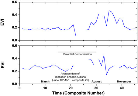
Figure 1. Missing values in the EVI time-series generated using the MODIS MOD09A1 product over two agricultural locations in Odisha, Eastern India in 2008. Missing values were detected using the MODIS quality assurance (QA) product; gaps in the time-series are where high-quality retrievals were not available to compute the EVI.

Issues in Phenology Profile Generation

Due to noise, multi-temporal remote sensing datasets exhibit local variation in spectral reflectance, and thus VI-values, punctuated by missing values (evident in Figure 1), whereas, over time, crop growth follows a smooth trajectory in normal conditions (events such as pest attacks, moisture shortage, natural disasters can perturb crop growth; see Sakamoto et al. (2007) for an example of mapping flood extent and duration in the Mekong Delta). To account for this several different approaches to filtering and smoothing raw remote sensing data are used to smooth remote sensing data to match an ideal crop growth profile. These approaches include Fourier transforms (Dash et al., 2010), Savitzky–Golay filters (Chen et al., 2004; Jonsson and Eklundh, 2004), logistic functions (Zhang et al., 2003), wavelet transforms (Sakamoto et al., 2005) or asymmetric Gaussian functions (Jonsson and Eklundh, 2004) amongst others. Hird and McDermid (2009) and Atkinson et al. (2012) provide comparisons of different smoothing approaches. Different smoothing techniques applied to the same raw remote sensing data can generate noticeable differences in crop growth dynamics, and, thus, detection of crop phenology. This is exemplified in Figure 2 which shows differences in rice crop growth profiles generated from the same raw data by Fourier and wavelet transforms.

FIGURE 2

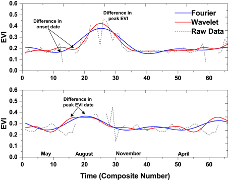
Figure 2. Smoothed phenology profiles, using Fourier and wavelet transforms, for the same pixels in Figure 1 (i.e., agricultural pixels in Odisha, Eastern India for the 2008–2009 cropping season. Annotations demonstrate how different smoothing techniques yield different start-of-season and peak VI retrievals. The time-series here has been extended to capture a potential second cropping season after the monsoon; the cropping season time-series displayed spans mid-March (pre-monsoon) in 2008 to the mid-May in 2009 (end of harvest of the post-monsoon crop).

Sakamoto et al. (2005) demonstrate the influence that different smoothing techniques have on estimating the timing of crop phenological development stages. This is evidenced in Figure 2 where there are clear differences in the timing and magnitude of peak VI and area under the curve, both proxy measures of crop productivity, yield, and biomass (Pettorelli et al., 2005; Funk and Budde, 2009). This source of error is particularly problematic in phenology-based approaches to yield gap analysis when shifts in the timing of crop development stages can have significant impacts on crop yield and influence crop sensitivity to climatic events (Lobell et al., 2012, 2013; Duncan et al., 2014a).

The phenological development stages observed from remote sensing data (such as onset of greenness and peak VI) are approximations of actual development stages that crops go through such as emergence, heading, anthesis, and grain filling. Numerous different approaches have been used across a range of studies and croplands to estimate the timing of crop development stages from VI derived crop phenology profiles (Jonsson and Eklundh, 2004; Sakamoto et al., 2005; Dash et al., 2010; Vrieling et al., 2011, 2013; Lobell et al., 2012, 2013). However, remote sensing does not measure directly the timing of specific crop development phases. Thus, approaches to estimate crop phenology from remote sensing data are typically not linked to environmental variables which drive crop development; often include calendar time as a predictor variable; are often arbitrary measures of crop green up, green down, and length of growing season; and susceptible to misdetection of a phenological transition (Brown and de Beurs, 2008).

Reflecting the above concerns, studies have sought to include environmental variables (such as temperature or relative humidity), which drive crop phenological development, into remote sensing based models of crop growth dynamics (De Beurs and Henebry, 2005; Brown and de Beurs, 2008; Duveiller et al., 2013). De Beurs and Henebry (2005) and Brown and de Beurs (2008) trained quadratic regression models expressing NDVI as a function of accumulated growing degree days (AGDD) and accumulated relative humidity (Arhum), respectively. Thus, crop development observed via VIs is not represented as a function of calendar time but of time crops are exposed to environmental variables which drive crop growth. In these models the intercept reflects crop greenness at low AGDD or Arhum, the slope parameter reflects the time (in units of AGDD or Arhum) to reach peak VI (or peak biomass), and the quadratic parameter determines the shape of the crop growth trajectory and length-of-season (De Beurs and Henebry, 2005). The advantage of these models are that they are tied to ecological theory and can be applied to VIs without the need for smoothing raw data (Brown and de Beurs, 2008). Duveiller et al. (2013) demonstrate that plotting multi-temporal LAI and green area index (GAI) (derived from MODIS and SPOT data) against AGDD over wheat croplands generates smoother crop trajectories than when plotted against calendar time.

However, the gains of incorporating environmental variables with remote sensing observations to estimate crop phenology is dependent upon understanding the environmental factors constraining (or driving) crop growth and development. For example, in some instances croplands are moisture-limited (Brown and de Beurs, 2008), temperature-limited (Lobell et al., 2012; Duncan et al., 2014a), or nutrient-limited (Tittonell and Giller, 2013). Therefore, identifying the correct environmental variables, or mix of environmental variables is critical to accurately modeling crop phenology. This is problematic in smallholder croplands on numerous counts due to the complex interplay of factors limiting crop growth, the spatial variability of these factors, and the availability of data required to resolve these issues at suitable spatio-temporal resolutions. Furthermore, the computation of AGDD is crop specific with regards to the values of the base temperature above which crop growth occurs and the values of critical temperatures which if exceeded are detrimental to crop growth (Hatfield et al., 2011; Gourdji et al., 2013; Teixeira et al., 2013). Also, a crop's sensitivity to temperature will vary throughout the growing season as it passes through different development stages (Hatfield et al., 2011). When computing AGDD for wheat croplands over Belgium Duveiller et al. (2013) do not specify a critical upper limit for temperature; if this method was directly applied in many of the smallholder croplands in the tropics it could miss out the harmful impact of extreme heat on crop growth (Lobell et al., 2012; Teixeira et al., 2013; Duncan et al., 2014a). Given the crop specific nature of these temperature values crop specific maps are required which are challenging to produce in heterogeneous smallholder croplands. Whilst linking environmental variables with remote sensing observations to monitor crop phenology offers a theoretical advance, its practical application in smallholder landscapes also remain challenging.

Approaches to estimating crop phenology from remote sensing, either using multi-temporal VIs in isolation or in combination with ancillary environmental variables, only enable estimates at the pixel level. In reality crop development phases occur at the plant scale which may not be universal across a pixel. Thus, it is difficult to validate the different approaches in the literature for estimating crop phenological parameters (Brown and de Beurs, 2008). Lobell et al. (2013) validated wheat crop start-of-season estimates, defined via a threshold approach, observed from EVI temporal profiles derived from MODIS using LAI generated from CERES crop simulation models. You et al. (2013) compared four approaches to estimate start-of-season and end-of-season with ground based measurements, across a range of crop types, in China; the four approaches were a 50% threshold between minimum and maximum NDVI (White and Nemani, 2006), curvature-change rate method (Zhang et al., 2003), maximum slope method (Yu et al., 2003), and threshold values for NDVI, slope of the NDVI temporal profile, and NDVI difference between NDVI at a given time-step and base (bare ground) NDVI trained using local observation data (You et al., 2013). All methods performed poorly in estimating end-of-season; however, for both start-of-season and end-of-season the thresholds trained with local observation data were the most accurate. Sakamoto et al. (2005) compared ground observations of planting date, heading date and harvesting date with estimates retrieved via inflection points and maximum values from MODIS EVI data smoothed via wavelet or Fourier transforms. Except for heading date, crop phenology retrievals from the wavelet transform had a noticeably lower root mean square error (RMSE) when compared to ground observations; however, Sakamoto et al. (2005) concluded the error in estimation dates was still too great for inclusion into crop simulation models. Brown and de Beurs (2008) compared start-of-season estimates derived from NDVI-Arhum regression models (trained using NDVI data from AVHRR, SPOT, and MODIS sensors) with rainfall based start-of-season estimates and farmer reported sowing and emergence dates. The NDVI based estimates were closer to farmer reported sowing and emergence dates than rainfall based estimates; start-of-season estimates based upon 8-day composites of MODIS data had a lower RMSE and a higher R² compared to 16-day MODIS composites and GIMMS AVHRR imagery when regressed against ground observations (Brown and de Beurs, 2008). However, Brown and de Beurs (2008) highlight sources of uncertainty in validating remote sensing-derived crop phenology: different farmers may have different interpretations of sowing or emergence dates, and averaging farmer reported sowing dates to a larger region may preclude the ability to validate the effect of image spatial resolution on crop phenology retrieval.

Thus, there is not a clear optimum approach to generating temporal profiles of crop growth or retrieving crop phenological parameters. This is compounded by challenges in validation, including: identifying what remote sensing-derived phenology metrics are observing, identifying suitable ground based metrics for validation, overcoming the different spatial scales at which satellite sensors observes crop growth dynamics and phenological developments occurring at the plant scale on the ground, and availability of ground based validation data over smallholder croplands. There is the potential that differences in methods used to generate crop growth dynamics from remote sensing data and to estimate crop phenological parameters will influence the results of yield gap analysis. It is important to be able to discriminate between observed yield variation which is real and yield variation which is an artifact of data processing and smoothing techniques.

Spatial Resolution

Typically, remote sensing-derived crop growth dynamics and phenology is monitored over croplands at a 250 m (Wardlow et al., 2007) or 500 m spatial resolution (Xiao et al., 2005, 2006) or with even coarser spatial resolutions (Rojas, 2007; Vrieling et al., 2011, 2013). This presents significant challenges in smallholder landscapes where average plot sizes can be far smaller than pixel sizes of the remote sensing data. For example, in Bihar, Odisha and Madhya Pradesh, some of India's poorest and most food insecure states (Menon et al., 2009; Pritchard et al., 2013), 91, 72, and 44%, respectively, of farm holdings are marginal (Ministry of Agriculture, 2014). At the national level in India, 67% of land holdings are marginal. Marginal holdings are less than 10,000 m² (Ministry of Agriculture, 2014). Whilst the majority of farmers in India have land holdings smaller than 10,000 m² the typical footprint of a 500 m gridded MODIS pixel is 250,000 m². Contrary to this, in the US. Great Central Plains where Wardlow et al. (2007) demonstrated that crop phenology can help discriminate crop types the field sizes are 325,000 m² or larger encompassing at least five 250 m spatial resolution MODIS pixels.

In smallholder landscapes this mismatch in scale is particularly problematic, firstly, the spatial resolution of pixels upon which spectral reflectance is recorded in gridded products (such as level 2G or level 3 MODIS or L1b and above MERIS products) will often cover a mix of land uses, fields and heterogeneous cropping patterns (Wolfe et al., 1998; Tan et al., 2006; Gómez-Chova et al., 2011). Thus, a single value (e.g., spectral reflectance, VI, LAI etc.) recorded within a pixel may mask locally important gradients in productivity and confound the ability to accurately estimate crop specific yield; this issue is clearly illustrated in the upper two panels of Figure 3 where one gridded MODIS pixel would encompass a mosaic of different fields and land cover types from ponds, forest, human settlement and fields. Furthermore, the pixels contained in gridded products, such as those depicted in Figure 3, are idealistic representations of the actual satellite sensor observation footprints (Wolfe et al., 1998; Tan et al., 2006; Duveiller et al., 2011; Gómez-Chova et al., 2011). The spatial resolutions of grid cells (for level 2G or level 3 MODIS products) and satellite sensor observation footprints will be the same at nadir, but observation footprint sizes will vary off-nadir, whereas pixel dimensions in grid cells will remain consistent across the landscape (Huang et al., 1998; Tan et al., 2006; Duveiller et al., 2011). For whiskbroom sensors, such as MODIS, the observation footprint increases with view zenith angle (Tan et al., 2006), but, misalignment and variation in observation footprints relative to uniform grids of processed products also impact pushbroom sensors, such as MERIS (Gómez-Chova et al., 2011). Thus, often, values in gridded pixels will be computed from a mix of radiance from adjacent regions which are also composed of a mix of land covers in smallholder croplands. This effect can be depicted by mapping observation coverage (obscov), which is the ratio of the intersection area, defined as the intersection area between the grid cell and the observation footprint, to the total area of the observation footprint (Tan et al., 2006). In the lower panel of Figure 3 the obscov is presented which illustrates the extent to which the area of the gridded pixel contributes to the observation value they report. Lobell (2013) highlights the problems of mixed land covers when using remote sensing in field scale yield gap analysis; he draws upon the challenge of generating accurate remote sensing estimates of crop yields in Sub-Saharan Africa where intercropping is common.

FIGURE 3

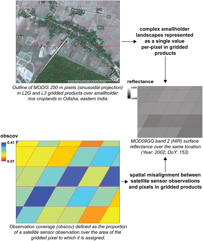
Figure 3. The upper panel depicts grid cell outlines, in Sinusoidal projection, from MODIS 250 m level 2G and 3 products over a smallholder landscape. The middle panel shows the corresponding spectral reflectance in the near-infrared wavelength reported for each grid cell in the MOD09GQ product. The bottom panel shows the observation coverage (obscov) values for the same grid cells. This image corresponds to smallholder croplands near the Bhitarkanika mangrove forests in Odisha, India (Sources: Esri, DigitalGlobe, GeoEye, i-cubed, Earthstar Geographics, CNES/Airbus DS, USDA, USGS, AEX, Getmapping, Aerogrid, IGN, IGP, swisstopo, and the GIS User Community).

When using coarse spatial resolution remote sensing data over relatively complex landscapes sampling methods have been proposed to select pixels of a specified purity (i.e., measured spectral reflectance is predominantly from a homogeneous land cover) for operational applications (e.g., monitoring crop development; Duveiller et al., 2008; Duveiller and Defourny, 2010). Over agricultural landscapes in Romania Duveiller et al. (2011) generate crop-specific, regional, multi-temporal profiles of GAI from MODIS 250 m imagery using pixel purity, observation coverage (obscov), and view zenith angle as criteria of selection for high quality, representative pixels. This approach has been extended to generate a longer-term time-series of GAI at the regional scale over croplands in Belgium (Duveiller et al., 2012), the ability to generate long-term data records offers advantages in being able to detect the occurrence of temporally persistent yield gaps and distinguish yield gaps from inter-annual yield variation (Lobell et al., 2010; Lobell, 2013).

In a similar vein, Bolton and Friedl (2013) discarded MODIS pixels with less than a 50% coverage of croplands and weighted the remaining pixel VI-values by the proportion of pixel cropland coverage when estimating crop yields. However, there are limitations to adopting these approaches in smallholder croplands. Monitoring crop growth and phenology from a sample of coarse spatial resolution pixels requires that enough pixels fall within fields; as discussed above pixel footprints from sensors with sufficient temporal resolution to resolve crop phenology are still coarse relative to the field dimensions in smallholder landscapes. Also, as demonstrated in Figure 4, using smallholder croplands in eastern India as an example, it is unlikely that there will be a large proportion of MODIS 500 m pixels with at least 50% cropland coverage. Furthermore, even if a pixel covers multiple fields of the same crop, in a smallholder landscape within-pixel variability will remain with regards to the timing of crop phenology, cultivars sown, management practices, and local gradients in crop yield (Tittonell and Giller, 2013). A recent map of global field sizes at a 1 km spatial resolution has been produced by Fritz et al. (2015) and is available at http://cropland.geo-wiki.org/; this product may open up opportunities for large-scale testing of how fragmented field patterns in smallholder landscapes confounds crop growth monitoring, phenology retrieval and subsequent yield estimation.

FIGURE 4

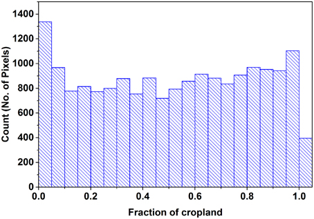
Figure 4. Histogram of cropland fraction in MODIS 500 m pixels derived from the MOD09A1 product over Jagatsinghpur and Kendrapara districts in Odisha, India. The cropland fraction within a MODIS 500 m pixel was derived from Landsat 30 m cropland map from the 2009 kharif rice growing season.

Sampling from a population of pixels, or discarding pixels based upon certain criteria reduces the ability to capture spatial variability in crop yields. For example, Funk and Budde (2009) and Bolton and Friedl (2013) aggregated yields estimated utilizing crop phenology derived from selected MODIS pixels to larger administrative units. The sampling, or selection, of high-quality MODIS observations to estimate crop-specific biophysical parameters captures regional growth dynamics (Duveiller and Defourny, 2010; Duveiller et al., 2011, 2012). However, such sampling approaches from moderate spatial resolution imagery come at the expense of the required spatial detail to observe local yield variability in smallholder croplands; often yield gaps will occur within the pixel footprints of moderate resolution sensors or will occur in pockets across a landscape which sampling approaches may fail to detect. Whilst these approaches are useful for inter-regional assessments of yield gaps they cannot reveal intra-regional or local variability in yield. For smallholders this local variability in yield is often important where crop yields vary over small distances (Tittonell and Giller, 2013) and, where, due to non-linear returns on assets a “relatively” small change in crop yield can have significant implications for levels of wellbeing (Carter and Barrett, 2006; Tittonell, 2014). Furthermore, the mismatch between the spatial resolution at which it is possible to observe crop growth and phenology and the size of fields and landscape heterogeneity in smallholder systems makes it difficult to accurately estimate crop yield. This inhibits identification of intra-cropland yield gaps and has obvious implications for the operational uses of crop phenology derived from remote sensing in this context.

Reflecting the discussion above, the challenge of using crop phenology-based approaches to estimate crop yield in smallholder landscapes, based on the current spatial resolution of suitable remote sensing data is evident in Figure 5. In Figure 5, a crop phenology-based approach to estimate peak WDRVI and EVI-values (using 500 m spatial resolution MOD09A1 MODIS data) across a smallholder rice cropping landscape in coastal Odisha, eastern India, captures a small amount of variation in rice crop yield (R² = 0.45 and 0.15, respectively). The method used to estimate rice crop yield here is similar to that employed by Bolton and Friedl (2013) over croplands in the USA; however, the relationship between EVI and maize and soybean yields in the USA approached R² = ~0.6. The distinction here is that these croplands are “intensive and extensive” with limited contamination from other land covers or mixed cropping mosaics (Bolton and Friedl, 2013, p. 76) compared to the predominantly small and marginal croplands of Odisha (Agriculture Department, 2013). The launch of Sentinel-2, and potential fusion with Landsat and other imagery, may overcome some of these limitations experienced by using current coarser spatial resolution remote sensing phenology products in smallholder croplands.

FIGURE 5

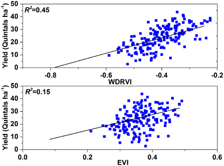
Figure 5. The relationship between block-wise kharif rice crop yields reported via agricultural statistics and block-wise weighted average peak WDRVI (upper panel) and EVI (lower panel) calculated using MODIS MOD09A1 data. The weight of each pixel's peak EVI in the calculation of block average peak EVI corresponds to the proportion of cropland within each pixel determined using two Landsat (30 m spatial resolution) crop maps (one from the 2002 kharif season and one from the 2009 kharif season). Here, only pixels with at least 50% cropland cover were retained for further analysis as in Bolton and Friedl (2013). Rice crop growing season and peak VI were extracted using a method similar to that outlined in Dash et al. (2010), but, with adapted thresholds. This analysis was performed for two districts (Jagatsinghpur and Kendrapara) in Odisha, India, from the 2001–2002 to the 2010–2011 cropping seasons.

Causation and Closure of Yield Gaps

Having identified where yield gaps exist, and estimated the magnitude of yield gaps, the next stage in the logical workflow to close yield gaps is to understand the underlying causes of underperforming fields. The timing of crop development stages, such as planting, anthesis, or grain filling can be correlated to final crop yield. Using phenology parameters (start-of-season and end-of-season) extracted from time-series of fAPAR derived from SPOT-VGT data over the Horn of Africa, Meroni et al. (2014) computed growing season cumulative sums of fAPAR (CfAPAR) as a proxy of gross primary production (GPP). Anomalies in CfAPAR from its average value at a location were used to detect drought, and the cause of such drought was identified through associated phenology parameters (e.g., late start-of-season shortening growing season length). It should be noted that detection of drought induced shortfalls in crop production is distinct from observing temporally persistent yield gaps; but such an approach could be adapted to identify where frequent droughts can contribute to long-term cropland underperformance. Lobell et al. (2013) observed yield declines for later sown crops using crop phenology derived from MODIS data for the wheat crop in north-west India.

Further studies have correlated crop phenology observed over wheat croplands in North-west India croplands with spatial grids of temperature data to explain patterns in crop yield declines (Lobell et al., 2012; Duncan et al., 2014a). These studies showed that earlier sowing decreased the exposure of crops to the periods of highest temperatures, and, identified which temperature variables influence crop performance. In this instance, remote sensing-derived crop phenology can be used to identify and explain the causes of yield gaps and suggest a remedy: earlier sowing. One route to achieving earlier sowing in North-west India is through zero-tillage; whilst zero-tillage may not result in increasing potential yields it can provide other benefits to farmers through reduced input costs (e.g., machine hire and fuel), reduced exposure to extreme heat events, and more sustainable agro-ecosystems (especially if zero-tillage is combined with other resource conserving practices; Gupta and Seth, 2007; Erenstein and Laxmi, 2008). This suggests that even if yield gaps are not closed per se; utilizing crop phenology to help target resource conserving practices can still yield benefits to smallholders. There is need for certain qualifications here; it has been suggested that moves toward conservation agriculture will not be universally beneficial for all smallholders; Giller et al. (2009) discuss the limitations of conservation agriculture in smallholder farming systems in Africa.

What the studies by Lobell et al. (2012) and Duncan et al. (2014a) also demonstrate is the potential to correlate crop phenological information with other spatial data to explore causes of yield gaps. Exploring the constraints of climatic variables on crop yields lends itself to this form of analysis given spatial gradients in rainfall and temperature, the availability of gridded climatic data (e.g., WORLDCLIM: http://www.worldclim.org/; APHRODITE: http://www.chikyu.ac.jp/precip/) or the ease of interpolating station data to grids at different spatial resolutions (Hijmans et al., 2005; Xie et al., 2007; Yatagai et al., 2009; Yasutomi et al., 2011). Alongside integrating climatic data with crop phenology to explain causes of yield gaps, Franch et al. (2015) extend the methodology of Becker-Reshef et al. (2010) by utilizing temperature data to compute AGDD, the heat the plant is exposed to, to predict peak NDVI (over a month in advance) and forecast wheat crop yields approximately two and a half months prior to harvest in the USA, China, and Ukraine. Thus, the integration of climatic data and remote sensing-derived crop phenology offers potential to predict within-season underperformance in croplands. However, the Franch et al. (2015) study forecasts yield at the administrative unit level and is not applied to forecast local variability in crop yields typical of smallholder croplands.

Whilst this analysis may reveal that smallholder croplands co-occur with certain challenging climates for crop growth (Brown et al., 2010; Vrieling et al., 2011); often, yield gaps exist within smallholder croplands and are explained by a range of, interacting, complex factors (Tittonell and Giller, 2013; Dzanku et al., 2015). For remote sensing-derived crop growth monitoring and phenology to shed light on the complex causes of yield gaps in smallholder croplands it must be compatible with a range of datasets from different disciplines. Lobell et al. (2002) combined multi-date maps of crop yield derived from 30 m spatial resolution Landsat imagery with soil type zone maps to explore the constraints on yield. Crop yields were grouped based on soil type and climate (determined by multi-date imagery capturing inter-annual climate variation); a statistical approach was then determined to explore the influence of between-group effects (e.g., soil type) vs. within-group effects (e.g., farmer-specific management practices) on crop yield. This work highlighted that most variation in crop yields was explained by within-group effects, highlighting the significant control of management practices on field-to-field crop yield as opposed to larger scale gradients corresponding to soil type. It was also shown that different management practices resulted in differential sensitivity to climate impacts upon yield. Field-to-field variability in yield can also be explained by soil quality, but at this scale this is likely to be the result of legacies of farm management decisions (Lobell et al., 2002; Tittonell and Giller, 2013). As mentioned, a recent advance is the generation of a global map of field sizes at a 1 km spatial resolution (Fritz et al., 2015) which could be coupled with spatial estimates of crop yield to assess what constraints field sizes are to realizing potential yields. This would open doors to large-scale testing of whether, and where, achieving economies of scale with regards to plot sizes and associated input/output factors presents barriers to farmers increasing their production.

As discussed in Section Spatial Resolution, the spatial resolution at which crop phenology can be estimated reliably with remote sensing data inhibits its use at the field scale in smallholder settings. Thus, whilst a phenology-based approach to monitoring local yield gaps remains limited in this context it will also be unable to help unpick the drivers of yield gaps. It is worth noting that single date per growing season Landsat images were used as inputs in the study by Lobell et al. (2002). There are further limitations in the utility of the use of the current state-of-the-art in remote sensing of crop growth and phenology retrieval over smallholder croplands. Firstly, there is a requirement for adequate ancillary datasets to correlate with crop phenology data; if these datasets are not available or of insufficient quality it reduces the explanatory value of the phenological information. Secondly, if crop phenological information can aid detection of local gradients in crop yield it does not explain what factor, or interaction of factors, is driving this variation. These factors can include fertilizer application, livestock interactions, soil salinity, cultivar type, pests, labor availability, behavioral choices by farmers, irrigation access and type, local institutions, road access, and past legacies of management (Tyagi et al., 2005; Lobell et al., 2010; Enfors, 2013; Tittonell and Giller, 2013; Tittonell, 2014). A location-specific understanding of these yield limiting factors is crucial to support effective policy and agricultural extension workers in delivering interventions which raise productivity on underperforming farms. Furthermore, smallholder farms and cropping landscapes are socio-ecological systems (Enfors, 2013) where farm productivity and potential productivity display complex and non-linear responses to inputs and management (Tittonell, 2014). Therefore, effective yield-gap-closing interventions need to be sensitive to local complexity, non-linear dynamics and the wider socio-economic and cultural context (Enfors, 2013). For example, Enfors (2013) highlighted how water management and conservation tillage interventions have little impact in fields unless they are coupled with supportive nutrient, agronomic and institutional environments. Currently, the information contained within remote sensing observations of crop growth and phenology estimates is ill suited to supporting such agricultural interventions, either by farmers or extension officers, in smallholder landscapes.

As stated by Tittonell and Giller (2013) demarcating zones of fertility, and estimating the proportion of fields in degraded states which need long-term rehabilitation, within smallholder landscapes is crucial to determining the true extent of yield gaps. Given the large (and often unavailable) data requirements for estimating zones of fertility and locally occurring potential yields via surveys or crop simulation modeling in smallholder landscapes (Tittonell and Giller, 2013) the potential uses of crop phenology from remote sensing should not be discounted. Also, as remote sensing measures actual crop yield it offers advantages in predicting locally attainable yield over methods, such as experimental plots which may be located on the most productive land or crop simulation models which are constrained by local data requirements (Tittonell and Giller, 2013).

Looking Forward and Future Research

Whilst the current suite of typical remote sensing products to monitor crop growth and estimate phenology is limited (e.g., MODIS, SPOT-VGT) research should focus on testing the validity of innovative data fusion methods, such as STARFM which combine the fine spatial detail in Landsat imagery with the temporal detail in MODIS imagery over smallholder landscapes (Gao et al., 2006; Lobell, 2013). The STARFM algorithm downscales MODIS spectral reflectance to a Landsat spatial resolution based upon a spatially weighted relationship between Landsat and MODIS spectral reflectance for a pair of images taken on similar dates (Gao et al., 2006). Other approaches to data fusion which generate “fine” spatial resolution, time-series to enable monitoring crop growth dynamics include linear-mixture models which exploit fine spatial detail in land-use/land-cover maps or fine resolution imagery with the spectral and temporal detail in moderate resolution imagery. Zurita-Milla et al. (2009) and Amorós-López et al. (2013) use linear mixture models to fuse Landsat imagery, MERIS imagery, and land-use/land-cover maps to compute VI and monitor crop growth dynamics and phenology at finer spatial resolutions. The STARFM approach to generating fine spatial resolution time-series of spectral reflectance is strengthened with increases in the numbers of temporally matching pairs of Landsat and MODIS imagery used as algorithm inputs (Gao et al., 2006; Watts et al., 2011). With Landsat 8 and Landsat 7 orbits designed to provide imagery every 8 days (Roy et al., 2014) it increases the likelihood of being able to match more Landsat and MODIS image pairs as inputs into data fusion algorithms. This in turn should enhance capabilities to generate finer spatial resolution temporal VI profiles over croplands. For all data fusion approaches there is a need for a quantitative evaluation of how effective data fusion techniques are in simulating fine spatial resolution crop growth, in estimating phenology, in enabling local yield, and yield gap estimates.

Furthermore, the upcoming launch of Sentinel-2 should strengthen the research agenda to explore ways to utilize crop phenology information over smallholder croplands. This could either be through using Sentinel-2 imagery in isolation, or combining it with Sentinel-3, MODIS, Landsat 8 or vector data via data fusion techniques. Looking forward, a strong theory of remote sensing of crop yield exists which new approaches to estimating remote sensing-derived crop phenology can draw upon. However, as demonstrated by Lobell et al. (2010) discriminating persistent yield gaps from inter-annual variability requires yield estimates from several years which presents problems with using Sentinel-2, or Sentinel-2 and Landsat 8 fusions, over more imminent time scales.

However, such a time-gap provides an opportunity to target research agendas before these products become operational in targeting and informing interventions to close yield gaps within smallholder croplands. Two key research agendas appear prominent, both linked to extensive validation relative to the context of application, i.e., the specific characteristics of smallholder croplands. Firstly, given the relatively “low” crop yields in many smallholder croplands it is important to ascertain whether real spatial variation in crop yield is distinguishable from error in crop yield estimates from new remote sensing products. Secondly, given the small field sizes and local landscape heterogeneity in smallholder croplands the extent to which the geometric accuracy (i.e., do satellite sensor observations correspond to gridded pixel outputs) of newly derived crop phenology retrievals confounds spatial targeting needs evaluation. If these two research agendas can be addressed then there is the potential to enhance the capability of using remote sensing to monitor crop growth and derive crop phenology measures to assist in increasing productivity within smallholder croplands.

Conclusions

This paper reviews the potential uses of crop phenology derived from remote sensing platforms in aiding yield gap assessments in smallholder cropping landscapes. Closing yield gaps in these contexts is a crucial step toward meeting required food demand and reducing food insecurity, with potential positive side effects for other development goals, such as poverty alleviation. Phenology-based approaches can increase the accuracy and thematic detail in crop area, crop type and cropping intensity classifications. The use of spatial-crop phenology information, when the correlation between spectral reflectance and crop yield varies through a growing season, has clear advantages for remote sensing-based yield estimation. These advantages have the potential to feed into and improve approaches to estimating yield gaps from remote sensing data.

However, most smallholder croplands are located in regions where obtaining reliable, repeat remote sensing observations is challenging due to atmospheric aerosols and cloud cover. Also, the spatial resolution at which remote sensing data is available to monitor crop growth dynamics and estimate phenology is too coarse to capture the heterogeneity and local variability of production in smallholder landscapes. These factors confound the use of phenological approaches to identifying yield gaps in smallholder contexts, especially when yield variation often occurs on a field-to-field basis. The spatial coverage of remote sensing-derived phenology datasets enables correlation with ancillary spatial datasets to explore the causes of yield gaps. However, this approach is undermined by (1) the requirement for a detailed number of spatial datasets with sufficient local detail to capture the complex causation of yield gaps in smallholder contexts and (2) the poor performance of estimating crop phenology at the finer scales of yield variability within smallholder landscapes. Thus, on a theoretical level the information contained within crop phenology could assist remote sensing-based yield gap analysis. However, in smallholder landscapes the characteristics of available remote sensing data used to estimate crop phenology is ill suited to yield gap identification or explanation.

The current state of remote sensing-derived crop phenology estimation can add value to yield gap assessments within larger, intensive, homogeneous croplands, such as those in the USA or north-west India. Given the global spatio-temporal coverage of MODIS and similar products crop phenological information can assist yield gap assessments between regions. However, the accuracy and applied value of remote sensing-derived crop phenology information within smallholder croplands must be treated with caution.

Author Contributions

JMAD, JD, and PA all contributed to the conception and drafting of this manuscript.

Conflict of Interest Statement

The authors declare that the research was conducted in the absence of any commercial or financial relationships that could be construed as a potential conflict of interest.

Acknowledgments

The authors would like to acknowledge the Leverhulme Trust who provides funds for JMAD and JD. PA is grateful to the University of Utrecht for supporting him with The Belle van Zuylen Chair.

References

Agriculture Department. (2013). State Agricultural Policy. Bhubaneswar.

Amorós-López, J., Gómez-Chova, L., Alonso, L., Guanter, L., Zurita-Milla, R., Moreno, J., et al. (2013). Multitemporal fusion of Landsat/TM and ENVISAT/MERIS for crop monitoring. Int. J. Appl. Earth Obs. Geoinf. 23, 132–141. doi: 10.1016/j.jag.2012.12.004

CrossRef Full Text | Google Scholar

Atkinson, P. M., Jeganathan, C., Dash, J., and Atzberger, C. (2012). Inter-comparison of four models for smoothing satellite sensor time-series data to estimate vegetation phenology. Remote Sens. Environ. 123, 400–417. doi: 10.1016/j.rse.2012.04.001

CrossRef Full Text | Google Scholar

Atzberger, C. (2013). Advances in remote sensing of agriculture: context description, existing operational monitoring systems and major information needs. Remote Sens. 5, 949–981. doi: 10.3390/rs5020949

CrossRef Full Text | Google Scholar

Barrett, C. B., and Constas, M. A. (2014). Toward a theory of resilience for international development applications. Proc. Natl. Acad. Sci. U.S.A. 111, 14625–14630. doi: 10.1073/pnas.1320880111

PubMed Abstract | CrossRef Full Text | Google Scholar

Bastiaanssen, W. G. M., and Ali, S. (2003). A new crop yield forecasting model based on satellite measurements applied across the Indus Basin, Pakistan. Agric. Ecosyst. Environ. 94, 321–340. doi: 10.1016/S0167-8809(02)00034-8

CrossRef Full Text | Google Scholar

Becker-Reshef, I., Vermote, E., Lindeman, M., and Justice, C. (2010). A generalized regression-based model for forecasting winter wheat yields in Kansas and Ukraine using MODIS data. Remote Sens. Environ. 114, 1312–1323. doi: 10.1016/j.rse.2010.01.010

CrossRef Full Text | Google Scholar

Biradar, C. M., and Xiao, X. (2011). Quantifying the area and spatial distribution of double- and triple-cropping croplands in India with multi-temporal MODIS imagery in 2005. Int. J. Remote Sens. 32, 367–386. doi: 10.1080/01431160903464179

CrossRef Full Text | Google Scholar

Bolton, D. K., and Friedl, M. A. (2013). Forecasting crop yield using remotely sensed vegetation indices and crop phenology metrics. Agric. For. Meteorol. 173, 74–84. doi: 10.1016/j.agrformet.2013.01.007

CrossRef Full Text | Google Scholar

Brown, M. E., and de Beurs, K. M. (2008). Evaluation of multi-sensor semi-arid crop season parameters based on NDVI and rainfall. Remote Sens. Environ. 112, 2261–2271. doi: 10.1016/j.rse.2007.10.008

CrossRef Full Text | Google Scholar

Brown, M. E., de Beurs, K., and Vrieling, A. (2010). The response of African land surface phenology to large scale climate oscillations. Remote Sens. Environ. 114, 2286–2296. doi: 10.1016/j.rse.2010.05.005

CrossRef Full Text | Google Scholar

Carter, M. R., and Barrett, C. B. (2006). The economics of poverty traps and persistent poverty: an asset-based approach. J. Dev. Stud. 42, 178–199. doi: 10.1080/00220380500405261

CrossRef Full Text | Google Scholar

Chakraborty, M., Panigrahy, S., and Sharma, S. A. (1997). Discrimination of rice crop grown under different cultural practices using temporal ERS-1 synthetic aperture radar data. ISPRS J. Photogramm. Remote Sens. 52, 183–191. doi: 10.1016/S0924-2716(97)00009-9

CrossRef Full Text | Google Scholar

Chen, J., Jonsson, P., Tamura, M., Gu, Z., Matsushita, B., and Eklundh, L. (2004). A simple method for reconstructing a high-quality NDVI time-series data set based on the Savitzky – Golay filter. Remote Sens. Environ. 91, 332–344. doi: 10.1016/j.rse.2004.03.014

CrossRef Full Text | Google Scholar

Das, S. R. (2012). Rice in Odisha. Los Banos, CA: International Rice Research Institute (IRRI). Available online at: http://books.irri.org/TechnicalBulletin16_content.pdf

Dash, J., Jeganathan, C., and Atkinson, P. M. (2010). Remote sensing of environment the use of MERIS terrestrial chlorophyll index to study spatio-temporal variation in vegetation phenology over India. Remote Sens. Environ. 114, 1388–1402. doi: 10.1016/j.rse.2010.01.021

CrossRef Full Text | Google Scholar

De Beurs, K. M., and Henebry, G. M. (2005). A statistical framework for the analysis of long image time series. Int. J. Remote Sens. 26, 1551–1573. doi: 10.1080/01431160512331326657

CrossRef Full Text | Google Scholar

De Wit, A., Duveiller, G., and Defourny, P. (2012). Estimating regional winter wheat yield with WOFOST through the assimilation of green area index retrieved from MODIS observations. Agric. For. Meteorol. 164, 39–52. doi: 10.1016/j.agrformet.2012.04.011

CrossRef Full Text | Google Scholar

Dente, L., Satalino, G., Mattia, F., and Rinaldi, M. (2008). Assimilation of leaf area index derived from ASAR and MERIS data into CERES-Wheat model to map wheat yield. Remote Sens. Environ. 112, 1395–1407. doi: 10.1016/j.rse.2007.05.023

CrossRef Full Text | Google Scholar

Doraiswamy, P. C., Sinclair, T. R., Hollinger, S., Akhmedov, B., Stern, A., and Prueger, J. (2005). Application of MODIS derived parameters for regional crop yield assessment. Remote Sens. Environ. 97, 192–202. doi: 10.1016/j.rse.2005.03.015

CrossRef Full Text | Google Scholar

Duncan, J. M. A., Dash, J., and Atkinson, P. M. (2014a). Elucidating the impact of temperature variability and extremes on cereal croplands through remote sensing. Glob. Chang. Biol. 21, 1541–1551. doi: 10.1111/gcb.12660

PubMed Abstract | CrossRef Full Text | Google Scholar

Duncan, J. M. A., Dash, J., and Atkinson, P. M. (2014b). Spatio-temporal dynamics in the phenology of croplands across the Indo-Gangetic Plains. Adv. Sp. Res. 54, 710–725. doi: 10.1016/j.asr.2014.05.003

CrossRef Full Text | Google Scholar

Duveiller, G., and Defourny, P. (2010). A conceptual framework to define the spatial resolution requirements for agricultural monitoring using remote sensing. Remote Sens. Environ. 114, 2637–2650. doi: 10.1016/j.rse.2010.06.001

CrossRef Full Text | Google Scholar

Duveiller, G., Baret, F., and Defourny, P. (2011). Crop specific green area index retrieval from MODIS data at regional scale by controlling pixel-target adequacy. Remote Sens. Environ. 115, 2686–2701. doi: 10.1016/j.rse.2011.05.026

CrossRef Full Text | Google Scholar

Duveiller, G., Baret, F., and Defourny, P. (2012). Remotely sensed green area index for winter wheat crop monitoring: 10-year assessment at regional scale over a fragmented landscape. Agric. For. Meteorol. 166–167, 156–168. doi: 10.1016/j.agrformet.2012.07.014

CrossRef Full Text | Google Scholar

Duveiller, G., Baret, F., and Defourny, P. (2013). Using thermal time and pixel purity for enhancing biophysical variable time series: an interproduct comparison. IEEE Trans. Geosci. Remote Sens. 51, 2119–2127. doi: 10.1109/TGRS.2012.2226731

CrossRef Full Text | Google Scholar

Duveiller, G., Defourny, P., and Gerard, B. (2008). “A method to determine the appropriate spatial resolution required for monitoring crop growth in a given agricultural landscape,” in Proceedings of the Geoscience and Remote Sensing Symposium, 2008. IGARSS 2008. IEEE International, Vol. 3 (Boston, MA), 562–565.

Google Scholar

Dzanku, F. M., Jirstrom, M., and Marstorp, H. (2015). Yield gap-based poverty gaps in rural Sub-Saharan Africa. World 67, 336–362. doi: 10.1016/j.worlddev.2014.10.030

CrossRef Full Text | Google Scholar

Enfors, E. I. (2013). Social–ecological traps and transformations in dryland agro-ecosystems: Using water system innovations to change the trajectory of development. Glob. Environ. Chang. 23, 51–60. doi: 10.1016/j.gloenvcha.2012.10.007

CrossRef Full Text | Google Scholar

Erenstein, O., and Laxmi, V. (2008). Zero tillage impacts in India's rice–wheat systems: a review. Soil Tillage Res. 100, 1–14. doi: 10.1016/j.still.2008.05.001

CrossRef Full Text | Google Scholar

ESA. (2010). GEMS Sentinel-2 Mission Documentation. Available online at: http://esamultimedia.esa.int/docs/GMES/Sentinel-2_MRD.pdf

FAO, IFAD, and WFP. (2012). The State of Food Insecurity in the World 2012. Economic Growth is Necessary but not Sufficient to Accelerate Reduction of Hunder and Malnutrition. Rome: FAO.

FAO, IFAD, and WFP. (2014). The State of Food Insecurity in the World. Strengthening the Enabling Environment for Food Security and Nutrition. Rome: FAO.

Foley, J. A., Ramankutty, N., Brauman, K. A., Cassidy, E. S., Gerber, J. S., Johnston, M., et al. (2011). Solutions for a cultivated planet. Nature 478, 337–342. doi: 10.1038/nature10452

PubMed Abstract | CrossRef Full Text | Google Scholar

Franch, B., Vermote, E. F., Becker-Reshef, I., Claverie, M., Huang, J., Zhang, J., et al. (2015). Improving the timeliness of winter wheat production forecast in the United States of America, Ukraine and China using MODIS data and NCAR Growing Degree Day information. Remote Sens. Environ. 161, 131–148. doi: 10.1016/j.rse.2015.02.014

CrossRef Full Text | Google Scholar

Fritz, S., See, L., McCallum, I., You, L., Bun, A., Moltchanova, E., et al. (2015). Mapping global cropland and field size. Glob. Chang. Biol. 21, 1980–1992. doi: 10.1111/gcb.12838

PubMed Abstract | CrossRef Full Text | Google Scholar

Funk, C., and Budde, M. E. (2009). Phenologically-tuned MODIS NDVI-based production anomaly estimates for Zimbabwe. Remote Sens. Environ. 113, 115–125. doi: 10.1016/j.rse.2008.08.015

CrossRef Full Text | Google Scholar

Ganguly, S., Friedl, M. A., Tan, B., Zhang, X., and Verma, M. (2010). Land surface phenology from MODIS: Characterization of the Collection 5 global land cover dynamics product. Remote Sens. Environ. 114, 1805–1816. doi: 10.1016/j.rse.2010.04.005

CrossRef Full Text | Google Scholar

Gao, F., Masek, J., Schwaller, M., and Hall, F. (2006). On the blending of the landsat and MODIS surface reflectance: predicting daily landsat surface reflectance. IEEE Trans. Geosci. Remote Sens. 44, 2207–2218. doi: 10.1109/TGRS.2006.872081

CrossRef Full Text | Google Scholar

Giller, K. E., Witter, E., Corbeels, M., and Tittonell, P. (2009). Conservation agriculture and smallholder farming in Africa: the heretics' view. F. Crop. Res. 114, 23–34. doi: 10.1016/j.fcr.2009.06.017

CrossRef Full Text | Google Scholar

Gitelson, A. A. (2004). Wide dynamic range vegetation index for remote quantification of biophysical characteristics of vegetation. J. Plant Physiol. 161, 165–173. doi: 10.1078/0176-1617-01176

PubMed Abstract | CrossRef Full Text | Google Scholar

Godfray, C. H. J., and Garnett, T. (2014). Food security and sustainable intensification. Philos. Trans. R. Soc. 369:20120273. doi: 10.1098/rstb.2012.0273

PubMed Abstract | CrossRef Full Text | Google Scholar

Gómez-Chova, L., Zurita-Milla, R., Alonso, L., Amorós-López, J., Guanter, L., and Camps-Valls, G. (2011). Gridding artifacts on medium-resolution satellite image time series: MERIS case study. IEEE Trans. Geosci. Remote Sens. 49, 2601–2611. doi: 10.1109/TGRS.2011.2108660

CrossRef Full Text | Google Scholar

Gourdji, S. M., Sibley, A. M., and Lobell, D. B. (2013). Global crop exposure to critical high temperatures in the reproductive period: historical trends and future projections. Environ. Res. Lett. 8, 024041. doi: 10.1088/1748-9326/8/2/024041

CrossRef Full Text | Google Scholar

Gumma, M. K., Nelson, A., Thenkabail, P. S., and Singh, A. N. (2011). Mapping rice areas of South Asia using MODIS multitemporal data. J. Appl. Remote Sens. 5, 053547. doi: 10.1117/1.3619838

CrossRef Full Text | Google Scholar

Gupta, R., and Seth, A. (2007). A review of resource conserving technologies for sustainable management of the rice-wheat cropping systems of the Indo-Gangetic plains (IGP). Crop Prot. 26, 436–447. doi: 10.1016/j.cropro.2006.04.030

CrossRef Full Text | Google Scholar

Harris, A., Carr, A. S., and Dash, J. (2014). Remote sensing of vegetation cover dynamics and resilience across southern Africa. Int. J. Appl. Earth Obs. Geoinf. 28, 131–139. doi: 10.1016/j.jag.2013.11.014

CrossRef Full Text | Google Scholar

Hatfield, J. L., Boote, K. J., Kimball, B. A., Ziska, L. H., Izaurralde, R. C., Ort, D., et al. (2011). Climate impacts on Agriculture: Impalications for Crop Production. Agron. J. 103, 351–370. doi: 10.2134/agronj2010.0303

CrossRef Full Text | Google Scholar

Hijmans, R. J., Cameron, S. E., Parra, J. L., Jones, P. G., and Jarvis, A. (2005). Very high resolution interpolated climate surfaces for global land areas. Int. J. Climatol. 25, 1965–1978. doi: 10.1002/joc.1276

CrossRef Full Text | Google Scholar

Hird, J. N., and McDermid, G. J. (2009). Noise reduction of NDVI time series: An empirical comparison of selected techniques. Remote Sens. Environ. 113, 248–258. doi: 10.1016/j.rse.2008.09.003

CrossRef Full Text | Google Scholar

HLPE. (2013). Investing in Smallholder Agriculture for Food Security. Rome. Available online at: http://www.fao.org/

Huang, C., Kalluri, S. N. V., Townshend, J. R. G., and Yang, K. (1998). Assessing and deconvolving the impacts of the point spread function on satellite remote sensing. Geosci. Remote Sens. Symp. 1998, 2035–2037.

Google Scholar

Huang, J., Wang, X., Li, X., Tian, H., and Pan, Z. (2013). Remotely sensed rice yield prediction using multi-temporal NDVI data derived from NOAA's-AVHRR. PLoS ONE 8:e70816. doi: 10.1371/journal.pone.0070816

PubMed Abstract | CrossRef Full Text | Google Scholar

Huete, A., Didan, K., Miura, T., Rodriguez, E. P., Gao, X., and Ferreira, L. G. (2002). Overview of the radiometric and biophysical performance of the MODIS vegetation indices. Remote Sens. Environ. 83, 195–213. doi: 10.1016/S0034-4257(02)00096-2

CrossRef Full Text | Google Scholar

Jiang, Z., Huete, A. R., Chen, J., Chen, Y., Li, J., Yan, G., et al. (2006). Analysis of NDVI and scaled difference vegetation index retrievals of vegetation fraction. Remote Sens. Environ. 101, 366–378. doi: 10.1016/j.rse.2006.01.003

CrossRef Full Text | Google Scholar

Jonsson, P., and Eklundh, L. (2004). TIMESAT—a program for analyzing time-series of satellite sensor data $. Comput. Geosci. 30, 833–845. doi: 10.1016/j.cageo.2004.05.006

CrossRef Full Text | Google Scholar

Li, Y., Liao, Q., Li, X., Liao, S., Chi, G., and Peng, S. (2003). Towards an operational system for regional-scale rice yield estimation using a time-series of Radarsat ScanSAR images. Int. J. Remote Sens. 24, 4207–4220. doi: 10.1080/0143116031000095970

CrossRef Full Text | Google Scholar

Licker, R., Johnston, M., Foley, J. A., Barford, C., Kucharik, C. J., Monfreda, C., et al. (2010). Mind the gap: How do climate and agricultural management explain the “yield gap” of croplands around the world? Glob. Ecol. Biogeogr. 19, 769–782. doi: 10.1111/j.1466-8238.2010.00563.x

CrossRef Full Text | Google Scholar

Lobell, D. B. (2013). The use of satellite data for crop yield gap analysis. F. Crop. Res. 143, 56–64. doi: 10.1016/j.fcr.2012.08.008

CrossRef Full Text | Google Scholar

Lobell, D. B., and Asner, G. (2004). Cropland distributions from temporal unmixing of MODIS data. Remote Sens. Environ. 93, 412–422. doi: 10.1016/j.rse.2004.08.002

CrossRef Full Text | Google Scholar

Lobell, D. B., Asner, G. P., Ortiz-Monasterio, J. I., and Benning, T. L. (2003). Remote sensing of regional crop production in the Yaqui Valley, Mexico: estimates and uncertainties. Agric. Ecosyst. Environ. 94, 205–220. doi: 10.1016/S0167-8809(02)00021-X

CrossRef Full Text | Google Scholar

Lobell, D. B., Cassman, K. G., and Field, C. B. (2009). Crop yield gaps: their importance, magnitudes, and causes. Annu. Rev. Environ. Resour. 34, 179–204. doi: 10.1146/annurev.environ.041008.093740

CrossRef Full Text | Google Scholar

Lobell, D. B., Ortiz-Monasterio, J. I., Addams, C. L., and Asner, G. P. (2002). Soil, climate, and management impacts on regional wheat productivity in Mexico from remote sensing. Agric. For. Meteorol. 114, 31–43. doi: 10.1016/S0168-1923(02)00138-7

CrossRef Full Text | Google Scholar

Lobell, D. B., Ortiz-Monasterio, J. I., and Falcon, W. P. (2007). Yield uncertainty at the field scale evaluated with multi-year satellite data. Agric. Syst. 92, 76–90. doi: 10.1016/j.agsy.2006.02.010

CrossRef Full Text | Google Scholar

Lobell, D. B., Ortiz-Monasterio, J. I., and Lee, A. S. (2010). Satellite evidence for yield growth opportunities in Northwest India. F. Crop. Res. 118, 13–20. doi: 10.1016/j.fcr.2010.03.013

CrossRef Full Text | Google Scholar

Lobell, D. B., Ortiz-Monasterio, J. I., Sibley, A. M., and Sohu, V. S. (2013). Satellite detection of earlier wheat sowing in India and implications for yield trends. Agric. Syst. 115, 137–143. doi: 10.1016/j.agsy.2012.09.003

CrossRef Full Text | Google Scholar

Lobell, D. B., Sibley, A., and Ortiz-monasterio, J. I. (2012). Extreme heat effects on wheat senescence in India. Nat. Clim. Chang. 2, 186–189. doi: 10.1038/nclimate1356

CrossRef Full Text | Google Scholar

Menon, P., Deolalikar, A., and Bhaskar, A. (2009). India State Hunger Index: Comparisons of Hunger across States. Washington, DC: Bonn and Riverside.

Meroni, M., Verstraete, M. M., Rembold, F., Urbano, F., and Kayitakire, F. (2014). A phenology-based method to derive biomass production anomalies for food security monitoring in the Horn of Africa. Int. J. Remote Sens. 35, 2472–2492. doi: 10.1080/01431161.2014.883090

CrossRef Full Text | Google Scholar

Ministry of Agriculture. (2014). All India Report on Number and Area of Operational Holdings. New Delhi. Available online at: http://dati.istat.it/

Mkhabela, M. S., Bullock, P., Raj, S., Wang, S., and Yang, Y. (2011). Crop yield forecasting on the Canadian Prairies using MODIS NDVI data. Agric. For. Meteorol. 151, 385–393. doi: 10.1016/j.agrformet.2010.11.012

CrossRef Full Text | Google Scholar

Mueller, N. D., Gerber, J. S., Johnston, M., Ray, D. K., Ramankutty, N., and Foley, J. A. (2012). Closing yield gaps through nutrient and water management. Nature 490, 254–257. doi: 10.1038/nature11420

PubMed Abstract | CrossRef Full Text | Google Scholar

Pettorelli, N., Vik, J. O., Mysterud, A., Gaillard, J.-M., Tucker, C. J., and Stenseth, N. C. (2005). Using the satellite-derived NDVI to assess ecological responses to environmental change. Trends Ecol. Evol. 20, 503–510. doi: 10.1016/j.tree.2005.05.011

PubMed Abstract | CrossRef Full Text | Google Scholar

Pinter, P. J., Jackson, R. D., Idso, S. B., and Reginato, R. J. (1981). Multidate spectral reflectance as predictors of yield in water stressed wheat and barley. Int. J. Remote Sens. 2, 43–48. doi: 10.1080/01431168108948339

CrossRef Full Text | Google Scholar

Pritchard, B., Rammohan, A., Sekher, M., Parasuraman, S., and Choithani, C. (2013). Feeding India: Livelihoods, Entitlements and Capabilities. Oxon: Routledge.

Google Scholar

Ramanathan, V., and Carmicheal, G. (2008). Global and regional climate changes due to black carbon. Nat. Geosci. 1, 221–227. doi: 10.1038/ngeo156

CrossRef Full Text | Google Scholar

Rammohan, A., and Pritchard, B. (2014). The role of landholding as a determinant of food and nutrition insecurity in rural Myanmar. World Dev. 64, 597–608. doi: 10.1016/j.worlddev.2014.06.029

CrossRef Full Text | Google Scholar

Ray, D. K., Mueller, N. D., West, P. C., and Foley, J. A. (2013). Yield trends are insufficient to double global crop production by 2050. PLoS ONE 8:e66428. doi: 10.1371/journal.pone.0066428

PubMed Abstract | CrossRef Full Text | Google Scholar

Rembold, F., Atzberger, C., Savin, I., and Rojas, O. (2013). Using low resolution satellite imagery for yield prediction and yield anomaly detection. Remote Sens. 5, 1704–1733. doi: 10.3390/rs5041704

CrossRef Full Text | Google Scholar

Rockström, J., Steffen, W., Noone, K., Lambin, E., Lenton, T. M., Scheffer, M., et al. (2009). Planetary boundaries: exploring the safe operating space for humanity. Ecol. Soc. 14, 32. Available online at: http://www.ecologyandsociety.org/vol14/iss2/art32/

PubMed Abstract

Rojas, O. (2007). Operational maize yield model development and validation based on remote sensing and agro-meteorological data in Kenya. Int. J. Remote Sens. 28, 3775–3793. doi: 10.1080/01431160601075608

CrossRef Full Text | Google Scholar

Rojas, O., Vrieling, A., and Rembold, F. (2011). Assessing drought probability for agricultural areas in Africa with coarse resolution remote sensing imagery. Remote Sens. Environ. 115, 343–352. doi: 10.1016/j.rse.2010.09.006

CrossRef Full Text | Google Scholar

Roy, D. P., Wulder, M. A., Loveland, T. R., Woodcock, C. E., Allen, R. G., Anderson, M. C., et al. (2014). Landsat-8: science and product vision for terrestrial global change research. Remote Sens. Environ. 145, 154–172. doi: 10.1016/j.rse.2014.02.001

CrossRef Full Text | Google Scholar

Sabates-Wheeler, R., and Devereux, S. (2011). Transforming Livelihoods for Resilient Futures: How to Facilitate Graduation in Social Protection Programmes. Brighton: Institute of Development Studies (IDS).

Google Scholar

Sakamoto, T., Gitelson, A. A., and Arkebauer, T. J. (2013). MODIS-based corn grain yield estimation model incorporating crop phenology information. Remote Sens. Environ. 131, 215–231. doi: 10.1016/j.rse.2012.12.017

CrossRef Full Text | Google Scholar

Sakamoto, T., Van Nguyen, N., Kotera, A., Ohno, H., Ishitsuka, N., and Yokozawa, M. (2007). Detecting temporal changes in the extent of annual flooding within the Cambodia and the Vietnamese Mekong Delta from MODIS time-series imagery. Remote Sens. Environ. 109, 295–313. doi: 10.1016/j.rse.2007.01.011

CrossRef Full Text | Google Scholar

Sakamoto, T., Yokozawa, M., Toritani, H., Shibayama, M., Ishitsuka, N., and Ohno, H. (2005). A crop phenology detection method using time-series MODIS data. 96, 366–374. doi: 10.1016/j.rse.2005.03.008

CrossRef Full Text | Google Scholar

Sen, A. (1981). Poverty and Famines. New York, NY: Oxford University Press.

Google Scholar

Shao, Y., Fan, X., Liu, H., Xiao, J., Ross, S., Brisco, B., et al. (2001). Rice monitoring and production estimation using multitemporal RADARSAT. Remote Sens. Environ. 76, 310–325. doi: 10.1016/S0034-4257(00)00212-1

CrossRef Full Text | Google Scholar

Smith, P. (2013). Delivering food security without increasing pressure on land. Glob. Food Sec. 2, 18–23. doi: 10.1016/j.gfs.2012.11.008

CrossRef Full Text | Google Scholar

Son, N. T., Chen, C. F., Chen, C. R., Minh, V. Q., and Trung, N. H. (2014). A comparative analysis of multitemporal MODIS EVI and NDVI data for large-scale rice yield estimation. Agric. For. Meteorol. 197, 52–64. doi: 10.1016/j.agrformet.2014.06.007

CrossRef Full Text | Google Scholar

Tan, B., Woodcock, C. E., Hu, J., Zhang, P., Ozdogan, M., Huang, D., et al. (2006). The impact of gridding artifacts on the local spatial properties of MODIS data: implications for validation, compositing, and band-to-band registration across resolutions. Remote Sens. Environ. 105, 98–114. doi: 10.1016/j.rse.2006.06.008

CrossRef Full Text | Google Scholar

Teixeira, E. I., Fischer, G., van Velthuizen, H., Walter, C., and Ewert, F. (2013). Global hot-spots of heat stress on agricultural crops due to climate change. Agric. For. Meteorol. 170, 206–215. doi: 10.1016/j.agrformet.2011.09.002

CrossRef Full Text | Google Scholar

Thenkabail, P. S., and Wu, Z. (2012). An automated cropland classification algorithm (ACCA) for Tajikistan by combining landsat, MODIS, and secondary Data. Remote Sens. 4, 2890–2918. doi: 10.3390/rs4102890

CrossRef Full Text | Google Scholar

Thenkabail, P. S., Biradar, C. M., Noojipady, P., Dheeravath, V., Li, Y., Velpuri, M., et al. (2009). Global irrigated area map (GIAM), derived from remote sensing, for the end of the last millennium. Int. J. Remote Sens. 30, 3679–3733. doi: 10.1080/01431160802698919

CrossRef Full Text | Google Scholar

Thenkabail, P. S., Gangadhararao, P., Biggs, T. W., Krishna, M., and Turral, H. (2007). Spectral matching techniques to determine historical land-use/land-cover (LULC) and irrigated areas using time-series 0. 1-degree AVHRR pathfinder datasets. Photogramm. Eng. Remote Sens. 73, 1029–1040. Available online at: http://info.asprs.org/publications/pers/2007journal/september/2007_sep_1029-1040.pdf

Tilman, D., Balzer, C., Hill, J., and Befort, B. L. (2011). Global food demand and the sustainable intensification of agriculture. Proc. Natl. Acad. Sci. U. S. A. 108, 20260–20264. doi: 10.1073/pnas.1116437108

PubMed Abstract | CrossRef Full Text | Google Scholar

Tittonell, P. (2014). Livelihood strategies, resilience and transformability in African. Agric. Syst. 126, 3–14. doi: 10.1016/j.agsy.2013.10.010

CrossRef Full Text | Google Scholar

Tittonell, P., and Giller, K. E. (2013). When yield gaps are poverty traps: the paradigm of ecological intensification in African smallholder agriculture. F. Crop. Res. 143, 76–90. doi: 10.1016/j.fcr.2012.10.007

CrossRef Full Text | Google Scholar

Tso, B., and Mather, P. M. (2009). Classification Methods for Remotely Sensed Data, 2nd Edn. Boca Raton, FL: CRC Press. doi: 10.1201/9781420090741

Google Scholar

Tucker, C. J. (1979). Red and photographic infrared l, lnear combinations for monitoring vegetation. Remote Sens. Environ. 150, 127–150. doi: 10.1016/0034-4257(79)90013-0

CrossRef Full Text | Google Scholar

Tyagi, N. K., Agrawal, A., Sakthivadivel, R., and Ambast, S. K. (2005). Water management decisions on small farms under scarce canal water supply: a case study from NW India. Agric. Water Manag. 77, 180–195. doi: 10.1016/j.agwat.2004.09.031

CrossRef Full Text | Google Scholar

Van Ittersum, M. K., Cassman, K. G., Grassini, P., Wolf, J., Tittonell, P., and Hochman, Z. (2013). Yield gap analysis with local to global relevance-a review. F. Crop. Res. 143, 4–17. doi: 10.1016/j.fcr.2012.09.009

CrossRef Full Text | Google Scholar

Vrieling, A., Beurs, K. M., and Brown, M. E. (2011). Variability of African farming systems from phenological analysis of NDVI time series. Clim. Change 109, 455–477. doi: 10.1007/s10584-011-0049-1

CrossRef Full Text | Google Scholar

Vrieling, A., De Leeuw, J., and Said, M. Y. (2013). Length of growing period over africa: Variability and trends from 30 years of NDVI time series. Remote Sens. 5, 982–1000. doi: 10.3390/rs5020982

CrossRef Full Text | Google Scholar

Wardlow, B. D., Egbert, S. L., and Kastens, J. H. (2007). Analysis of time-series MODIS 250m vegetation index data for crop classification in the U.S. Central Great Plains. Remote Sens. Environ. 108, 290–310. doi: 10.1016/j.rse.2006.11.021

CrossRef Full Text | Google Scholar

Wassmann, R., Jagadish, S. V. K., Heuer, S., Ismail, A., Redona, E., Serraj, R., et al. (2009). Climate change affecting rice production: the physiological and agronomic basis for possible adaptation strategies. Adv. Agron. 101, 59–122. doi: 10.1016/S0065-2113(08)00802-X

CrossRef Full Text | Google Scholar

Watts, J. D., Powell, S. L., Lawrence, R. L., and Hilker, T. (2011). Improved classification of conservation tillage adoption using high temporal and synthetic satellite imagery. Remote Sens. Environ. 115, 66–75. doi: 10.1016/j.rse.2010.08.005

CrossRef Full Text | Google Scholar

Whitcraft, A. K., Vermote, E. F., Becker-reshef, I., and Justice, C. O. (2015). Remote sensing of environment cloud cover throughout the agricultural growing season: impacts on passive optical earth observations. Remote Sens. Environ. 156, 438–447. doi: 10.1016/j.rse.2014.10.009

CrossRef Full Text | Google Scholar

White, M. A., and Nemani, R. R. (2006). Real-time monitoring and short-term forecasting of land surface phenology. Remote Sens. Environ. 104, 43–49. doi: 10.1016/j.rse.2006.04.014

CrossRef Full Text | Google Scholar

Wolfe, R. E., Roy, D. P., and Vermote, E. (1998). MODIS land data storage, gridding, and compositing methodology: Level 2 grid. IEEE Trans. Geosci. Remote Sens. 36, 1324–1338. doi: 10.1109/36.701082

CrossRef Full Text | Google Scholar

Xiao, X., Boles, S., Frolking, S., Li, C., Babu, J. Y., Salas, W., et al. (2006). Mapping paddy rice agriculture in South and Southeast Asia using multi-temporal MODIS images. Remote Sens. Environ. 100, 95–113. doi: 10.1016/j.rse.2005.10.004

CrossRef Full Text | Google Scholar

Xiao, X., Boles, S., Liu, J., Zhuang, D., Frolking, S., Li, C., et al. (2005). Mapping paddy rice agriculture in Southern China using multi-temporal MODIS images. Remote Sens. Environ. 95, 480–492. doi: 10.1016/j.rse.2004.12.009

CrossRef Full Text | Google Scholar

Xie, P., Chen, M., Yang, S., Yatagai, A., Hayasaka, T., Fukushima, Y., et al. (2007). A gauge-based analysis of daily precipitation over East Asia. J. Hydrometeorol. 8, 607–626. doi: 10.1175/JHM583.1

CrossRef Full Text | Google Scholar

Yasutomi, N., Hamada, A., and Yatagai, A. (2011). Development of a long-term daily gridded temperature dataset and its application to rain/snow discrimination of daily precipitation. Glob. Environ. Res. V15N2, 165–172. Available online at: http://www.chikyu.ac.jp/precip/data/Yasutomi2011GER.pdf

Yatagai, A., Arakawa, O., Kamiguchi, K., Kawamoto, H., Nodzu, M. I., and Hamada, A. (2009). A 44-year daily gridded precipitation dataset for asia based on a dense network of rain gauges. SOLA 5, 137–140. doi: 10.2151/sola.2009-035

CrossRef Full Text | Google Scholar

You, X., Meng, J., Zhang, M., and Dong, T. (2013). Remote sensing based detection of crop phenology for agricultural zones in China using a new threshold method. Remote Sens. 5, 3190–3211. doi: 10.3390/rs5073190

CrossRef Full Text | Google Scholar

Yu, F., Price, K. P., Ellis, J., and Shi, P. (2003). Response of seasonal vegetation development to climatic variations in eastern central Asia. Remote Sens. Environ. 87, 42–54. doi: 10.1016/S0034-4257(03)00144-5

CrossRef Full Text | Google Scholar

Zhang, X., Chen, S., Sun, H., Pei, D., and Wang, Y. (2008). Dry matter, harvest index, grain yield and water use efficiency as affected by water supply in winter wheat. Irrig. Sci. 27, 1–10. doi: 10.1007/s00271-008-0131-2

CrossRef Full Text | Google Scholar

Zhang, X., Friedl, M. A., Schaaf, C. B., Strahler, A. H., Hodges, J. C. F., Gao, F., et al. (2003). Monitoring vegetation phenology using MODIS. Remote Sens. Environ. 84, 471–475. doi: 10.1016/S0034-4257(02)00135-9

CrossRef Full Text | Google Scholar

Zurita-Milla, R., Kaiser, G., Clevers, J. G. P. W., Schneider, W., and Schaepman, M. E. (2009). Downscaling time series of MERIS full resolution data to monitor vegetation seasonal dynamics. Remote Sens. Environ. 113, 1874–1885. doi: 10.1016/j.rse.2009.04.011

CrossRef Full Text | Google Scholar