DeepTox: Toxicity Prediction using Deep Learning

1. Introduction

Humans are exposed to an abundance of chemical compounds via the environment, nutrition, cosmetics, and drugs. To protect humans from potentially harmful effects, these chemicals must pass reliable tests for adverse effects and, in particular, for toxicity. A compound's effects on human health are assessed by a large number of time- and cost-intensive in vivo or in vitro experiments. In particular, numerous methods rely on animal tests, trading off additional safety against ethical concerns. The aim of the “Toxicity testing in the Twenty-first century” initiative is to develop more efficient and less time-consuming approaches to predicting how chemicals affect human health (Andersen and Krewski, 2009; Krewski et al., 2010). The most efficient approaches employ computational models that can screen large numbers of compounds in a short time and at low costs (Rusyn and Daston, 2010). However, computational models often suffer from insufficient accuracy and are not as reliable as biological experiments. In order for computational models to replace biological experiments, they must achieve comparable accuracy. Within the “Tox21 Data Challenge” (Tox21 challenge), the performance of computational methods for toxicity testing was assessed in order to judge their potential to reduce in vitro experiments and animal testing.

The Tox21 challenge organizers invited participants to build computational models to predict the toxicity of compounds for 12 toxic effects (see Figure 1). These toxic effects comprised stress response effects (SR), such as the heat shock response effect (SR-HSE), and nuclear receptor effects (NR), such as activation of the estrogen receptor (NR-ER). Both SR and NR effects are highly relevant to human health, since activation of nuclear receptors can disrupt endocrine system function (Chawla et al., 2001; Grün and Blumberg, 2007), and activation of stress response pathways can lead to liver injury or cancer (Bartkova et al., 2005; Labbe et al., 2008; Jaeschke et al., 2012). For constructing computational models, high-throughput screening assay measurements of these twelve toxic effects were provided. The training set consisted of the Tox21 10K compound library, which includes environmental chemicals and drugs (Huang et al., 2014). For a set of 647 new compounds, computational models had to predict the outcome of the high-throughput screening assays (see Figure 1). The assay measurements for these test compounds were withheld from the participants and used to evaluate the performance of the computational methods. The “area under ROC curve” (AUC) was used as a performance criterion that reflects how well a method can rank toxic compounds higher than non-toxic compounds.

FIGURE 1

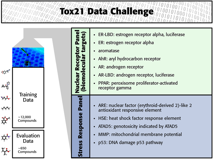
Figure 1. Overview of the Tox21 challenge dataset.

The participants in the Tox21 challenge used a broad range of computational methods for toxicity prediction, most of which were from the field of machine learning. These methods represent the chemical compound by chemical descriptors, the features, which are fed into a predictor. Methods for predicting biological effects are usually categorized into similarity-based approaches and feature-based approaches. Similarity-based methods compute a matrix of pairwise similarities between compounds which is subsequently used by the prediction algorithms. These methods, which are based on the idea that similar compounds should have a similar biological effect include nearest neighbor algorithms (e.g., Kauffman and Jurs, 2001; Ajmani et al., 2006; Cao et al., 2012) and support vector machines (SVMs, e.g., Mahé et al., 2005; Niu et al., 2007; Darnag et al., 2010). SVMs rely on a kernel matrix which represents the pairwise similarities of objects. In contrast to similarity based methods, feature based methods either select input features (chemical descriptors) or weight them by a score or a model parameter. Feature-based approaches include (generalized) linear models (e.g., Luco and Ferretti, 1997; Sagardia et al., 2013), random forests, (e.g., Svetnik et al., 2003; Polishchuk et al., 2009), and scoring schemes based on naive Bayes (Bender et al., 2004; Xia et al., 2004). Choosing informative features for the task at hand is key in feature-based methods and requires deep insights into chemical and biological properties and processes (Verbist et al., 2015), such as interactions between molecules (e.g., ligand-target), reactions and enzymes involved, and metabolic modifications of the molecules. Similarity-based approaches, in contrast, require a proper similarity measure between two compounds. The measure may use a feature-based, a 2D graph-based, or a 3D representation of the compound. Graph-based compound and molecule representations led to the invention of graph and molecule kernels (Kashima et al., 2003, 2004; Ralaivola et al., 2005; Mahé et al., 2006; Mohr et al., 2008; Vishwanathan et al., 2010; Klambauer et al., 2015). These methods are not able to automatically create task-specific or new chemical features. Deep Learning, however, excels in constructing new, task-specific features that result in data representations which enable Deep Learning methods to outperform previous approaches, as has been demonstrated in various speech and vision tasks.

Deep Learning (LeCun et al., 2015; Schmidhuber, 2015) has emerged as a highly successful field of machine learning. It has already impacted a wide range of signal and information processing fields, redefining the state of the art in vision (Cireşan et al., 2012a; Krizhevsky et al., 2012), speech recognition (Dahl et al., 2012; Deng et al., 2013; Graves et al., 2013), text understanding and natural language processing (Socher and Manning, 2013; Sutskever et al., 2014), physics (Baldi et al., 2014), and life sciences (Cireşan et al., 2013). MIT Technology Review selected it as one of the 10 technological breakthroughs of 2013. Deep Learning has already been applied to predict the outcome of biological assays (Dahl et al., 2014; Unterthiner et al., 2014, 2015; Ma et al., 2015), which made it our prime candidate for toxicity prediction.

Deep Learning is based on artificial neural networks with many layers consisting of a high number of neurons, called deep neural networks (DNNs). A formal description of DNNs is given in Section 2.2.1. In each layer Deep Learning constructs features in neurons that are connected to neurons of the previous layer. Thus, the input data is represented by features in each layer, where features in higher layers code more abstract input concepts (LeCun et al., 2015). In image processing, the first DNN layer detects features such as simple blobs and edges in raw pixel data (Lee et al., 2009; see Figure 2). In the next layers these features are combined to parts of objects, such as noses, eyes and mouths for face recognition. In the top layers the objects are assembled from features representing their parts such as faces.

FIGURE 2

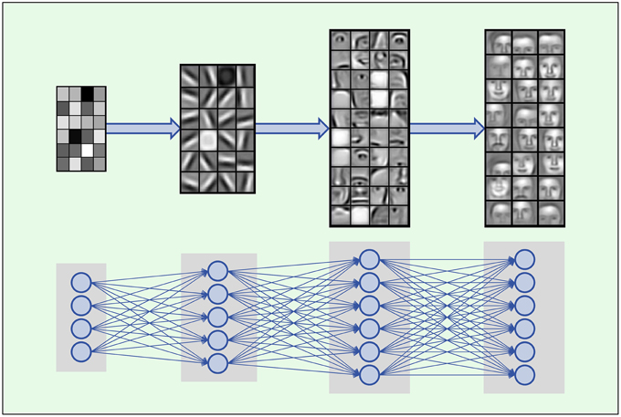
Figure 2. Hierarchical composition of complex features. DNNs build a feature from simpler parts. A natural hierarchy of features arises. Input neurons represent raw pixel values which are combined to edges and blobs in the lower layers. In the middle layers contours of noses, eyes, mouths, eyebrows and parts thereof are built, which are finally combined to abstract features such as faces. Images adopted from Lee et al. (2011) with permission from the authors.

The ability to construct abstract features makes Deep Learning well suited to toxicity prediction. The representation of compounds by chemical descriptors is similar to the representation of images by DNNs. In both cases the representation is hierarchical and many features within a layer are correlated. This suggests that Deep Learning is able to construct abstract chemical descriptors automatically. The constructed features can indicate functional groups or toxicophores (Kazius et al., 2005) as visualized in Figure 3.

FIGURE 3

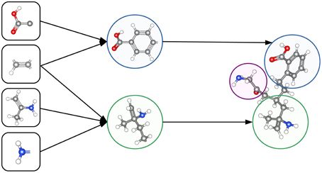
Figure 3. Representation of a toxicophore by hierarchically related features. Simple features share chemical properties coded as reactive centers. Combining reactive centers leads to toxicophores that represent specific toxicological effects.

The construction of indicative abstract features by Deep Learning can be improved by Multi-task learning. Multi-task learning incorporates multiple tasks into the learning process (Caruana, 1997). In the case of DNNs, different related tasks share features, which therefore capture more general chemical characteristics. In particular, multi-task learning is beneficial for a task with a small or imbalanced training set, which is common in computational toxicity. In this case, due to insufficient information in the training data, useful features cannot be constructed. However, multi-task learning allows this task to borrow features from related tasks and, thereby, considerably increases the performance.

Deep Learning thrives on large amounts of training data in order to construct indicative features (Krizhevsky et al., 2012) and, thereby, well-performing models. Recently, the availability of high-throughput toxicity assays provides sufficient data to use Deep Learning for toxicity prediction (Andersen and Krewski, 2009; Krewski et al., 2010; Shukla et al., 2010). In summary, Deep Learning is likely to perform well with the following prerequisites:

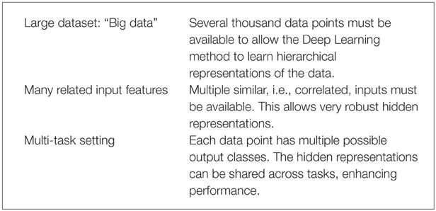
These three conditions are fulfilled for the Tox21 dataset: (1) High throughput toxicity assays have provided vast amounts of data. (2) Chemical compound descriptors are correlated. (3) A Multi-task setting is natural as different assays measure different but related toxic effects for the same compound (see Figure 4). To conclude, Deep Learning seems promising for computational toxicology because of its ability to construct abstract chemical features.

FIGURE 4

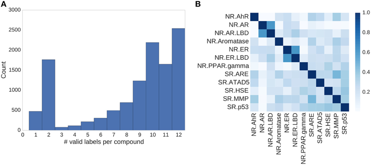
Figure 4. Assay correlation. (A) Histogram showing the number of unambiguous assay label assignments per compound. Only ≈500 compounds had a label for just one assay, more than half (54%) of the compounds had labels for 10 or more tasks. (B) Absolute correlation coefficient between the different assays of the Tox21 challenge.

2. Materials and Methods

For the Tox21 challenge, we used Deep Learning as key technology, for which we developed a prediction pipeline (DeepTox) that enables the use of Deep Learning for toxicity prediction. The DeepTox pipeline was developed for datasets with characteristics similar to those of the Tox21 challenge dataset and enables the use of Deep Learning for toxicity prediction. We first introduce the challenge dataset in Section 2.1. In Section 2.2 we then present, how we utilized Deep Learning for Toxicity prediction, while in Section 2.3 the DeepTox pipeline is explained.

2.1. Tox21 Challenge Data

In the Tox21 challenge, a dataset with 12,707 chemical compounds was given. This dataset consisted of a training dataset of 11,764, a leaderboard set of 296, and a test set of 647 compounds. For the training dataset, the chemical structures and assay measurements for 12 different toxic effects were fully available to the participants right from the beginning of the challenge, as were the chemical structures of the leaderboard set. However, the leaderboard set assay measurements were withheld by the challenge organizers during the first phase of the competition and used for evaluation in this phase, but were released afterwards, such that participants could improve their models with the leaderboard data for the final evaluation. Table 1 lists the number of active and inactive compounds in the training and the leaderboard sets of each assay. The final evaluation was done on a test set of 647 compounds, where only the chemical structures were made available. The assay measurements were only known to the organizers and had to be predicted by the participants. In summary, we had a training set consisting of 11,764 compounds, a leaderboard set consisting of 296 compounds, both available together with their corresponding assay measurements, and a test set consisting of 647 compounds to be predicted by the challenge participants (see Figure 1). The chemical compounds were given in SDF format, which contains the chemical structures as undirected, labeled graphs whose nodes and edges represent atoms and bonds, respectively. The outcomes of the measurements were categorized (i.e., that is labeled) as “active,” “inactive,” or “inconclusive/not tested.” Not all compounds were measured on all assays (see Figure 4A).

TABLE 1

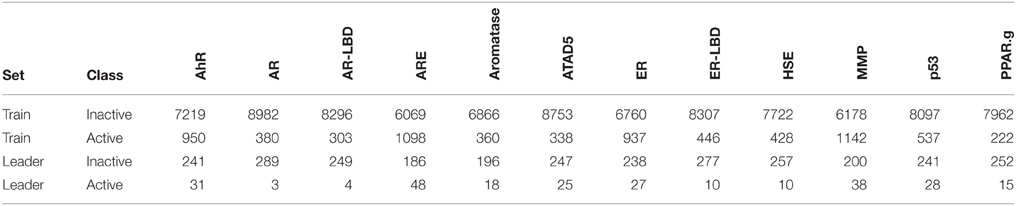
Table 1. Number of active and inactive compounds in the training (Train) and the leaderboard (Leader) sets of each assay.

2.2. Deep Learning for Toxicity Prediction

Deep Learning is a highly successful machine learning technique that has already revolutionized many scientific areas. Deep Learning comprises an abundance of architectures such as deep neural networks (DNNs) or convolutional neural networks. We propose a DNNs for toxicity prediction and present the method's details and algorithmic adjustments in the following. First we introduce neural networks, and in particular DNNs, in Section 2.2.1. In Section 2.2.2, we then discuss key techniques that led to the success of DNNs compared to shallow and small neural networks. The objective that was minimized for the DNNs for toxicity prediction and the corresponding optimization algorithms are discussed in Section 2.2.3. We explain DNN hyperparameters and the DNN architectures used in Section 2.2.4. In Section 2.2.5, we describe the hardware that was employed to optimize the objectives of the DeepTox DNNs.

2.2.1. Deep Neural Networks

A neural network, and a DNN in particular, can be considered as a function that maps an input vector to an output vector. The mapping is parameterized by weights that are optimized in a learning process. In contrast to shallow networks, which have only one hidden layer and only few hidden neurons per layer, DNNs comprise many hidden layers with a great number of neurons. A DNN may have thousands of neurons in each layer (Cireşan et al., 2012b), which is in contrast to traditional artificial neural networks, that employ only a small number of neurons. The goal is no longer to just learn the main pieces of information, but rather to capture all possible facets of the input.

A neuron can be considered as an abstract feature with a certain activation value that represents the presence of this feature. A neuron is constructed from neurons of the previous layer, that is, the activation of a neuron is computed from the activation of neurons one layer below. The first layer is the “input layer,” in which neuron activations are set to the value of the input vector. The last layer is the “output layer,” where the activations represent the output vector. The intermediate layers are the “hidden layers,” which give intermediate representations of the input vector.

Figure 5 visualizes the neural network mapping of an input vector to an output vector. A compound is described by the vector of its input features x. The neural network NN maps the input vector x to the output vector y. The activation value $h_j^l$ of a neuron j in a layer l of the neural network is computed as the weighted sum over the values $h_i^{l-1}$ of all neurons i in layer (l − 1), followed by the application of an activation function f. The weight $w_{ji}^l$ scales the activation $h_i^{l-1}$ of neuron i in layer (l − 1) before it is summed to compute the activation of neuron j in layer l. If the neural network has m layers, then the formulas are

$\begin{array}{l}y=\text{NN}(x),\hfill \\ h^0=x,\hfill \\ h_j^l=f({\displaystyle \sum _i}{w}_{ji}^l{h}_i^{l-1}),\hfill \\ y=h^m.\hfill \end{array}$

In matrix notation, the activation of neurons is

$h^l=f(W^l{h}^{l-1}).$

The output layer often has a special activation function, which is denoted by σ instead of f in Figure 5. Each neuron has a bias weight (i.e., a constant offset), that is added to the weighted sum for computing the activation of a neuron. To keep the notation uncluttered, these bias weights are not written explicitly, although they are model parameters like other weights.

FIGURE 5

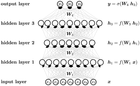
Figure 5. Schematic representation of a DNN.

2.2.2. Key Techniques for Deep Neural Networks

Recent algorithmic improvements in training DNNs enabled the success of Deep Learning: (1) “rectified linear units” (ReLUs) enforce sparse representations and counteract the vanishing gradient, (2) “dropout” for regularization, and (3) a cross-entropy objective combined with softmax or sigmoid activation.

One of the most successful inventions in the context of DNNs are rectified linear units (ReLUs) as activation functions (Nair and Hinton, 2010; Glorot et al., 2011). A ReLU f is the identity for positive values and zero otherwise. This activation function is called the “ramp function”:

$f\left(x\right)=\max \left(0,x\right).$

Using ReLUs in DNNs leads to sparse input representations, which are robust against noise and advantageous for classifiers because classification is more likely to be easier in higher-dimensional spaces (Ranzato et al., 2008). Probably the most important advantage of ReLUs is that they are a remedy for the vanishing gradient (Hochreiter, 1991; Hochreiter et al., 2000), from which networks with sigmoid activation functions and many layers suffer. “Vanishing” means in this context that the length of a gradient decreases exponentially when propagated through the layers, ultimately becoming too small for learning in the lower(/est) layers. Another enabling technique is “dropout,” which is one of the new regularization schemes that arose with the advent of DNNs in order to prevent overfitting—a serious problem for DNNs, as the number of hidden neurons is large and the complexity of the model class is very high. Dropout avoids co-adaption of units by randomly dropping units during training, that is, setting their activations and derivatives to zero (Hinton et al., 2012; Srivastava et al., 2014). The third technique that paved the way for the success of DNNs is the application of error functions such as cross-entropy and logistic-loss as objectives to be minimized. These error functions are combined with softmax or sigmoid activation functions in the output neurons.

2.2.3. DNN Learning, Objective and Optimization

The goal of neural network learning is to adjust the network weights such that the input-output mapping has a high predictive power on future data. We want to explain the training data, that is, to approximate the input-output mapping on the training data. Our goal is therefore to minimize the error between predicted and known outputs on that data. The training data consists of the output vector t for input vector x, where the input vector is represented using d chemical features, and the length of the output vector is n, the number of tasks. Let us consider a classification task. For classification, the output component t_k for task k is binary, that is, t_k ∈ {0, 1}. In the case of toxicity prediction, the tasks represent different toxic effects, where zero indicates the absence and one the presence of a toxic effect. The neural network predicts the outputs y_k. In the output layer of the neural network a sigmoid activation function is used. Therefore, the neural network predicts outputs y_k, that are between 0 and 1, and the training data are perfectly explained if for all training examples all outputs k are predicted correctly, i.e., y_k = t_k. To penalize non-matching output-target pairs, an error function or objective is defined. Minimizing this error function means better aligning network outputs and targets. Typically, the cross-entropy is used as an error function for multi-class classification. In our case, we deal with multi-task classification, where multiple outputs can be one (multiple different toxic effects for one compound) or none can be one (no toxic effect at all). For the multi-task setting we use a logistic error function −t_klog(y_k) − (1 − t_k)log(1 − y_k) for each output component k. If t_k = y_k, then only terms (1log1) or (0log0) appear, and the logistic error function is zero (note that (0log0) is defined to be zero). Otherwise, the logistic error function gives a positive value. The overall error function is the sum of these logistic error functions across all output components:

$-{\displaystyle \sum _{k=1}^n}{t}_k\log (y_k)+(1-t_k)\log (1-y_k).$

To cope with missing labels, we introduce a binary vector m for each sample, where m_k is one if the sample has a label for task k and zero otherwise. This leads to a slight modification to the above objective:

$-{\displaystyle \sum _{k=1}^n}{m}_k\left(t_k\log (y_k)+(1-t_k)\log (1-y_k)\right).$

Learning minimizes this objective with respect to the weights, as the outputs y_k are parametrized by the weights. The optimization problem is usually solved by gradient descent, which aims to minimize an objective function by iteratively adapting the parameters of the optimization problem in the direction of the steepest descent (the negative gradient) until a stationary point is found. A critical parameter is the step size or learning rate, i.e., how strongly the parameters are changed in the update direction. If a small step size is chosen, the parameters converge slowly to the local optimum. If the step size is too high, the parameters oscillate.

For neural networks, gradient descent can be applied with high computational efficiency by using the backpropagation algorithm (Werbos, 1974; Rumelhart et al., 1986). A computational simplification to computing a gradient over all training samples is stochastic gradient descent (Bottou, 2010). Stochastic gradient descent computes a gradient for an equally-sized set of randomly chosen training samples, a mini-batch, and updates the parameters according to this mini-batch gradient (Ngiam et al., 2011). The advantage of stochastic gradient descent is that the parameter updates are faster. The main disadvantage of stochastic gradient descent is that the parameter updates are more imprecise. For large datasets the increase in speed clearly outweighs the imprecision.

2.2.4. Hyperparameter Settings and DNN Network Architectures

The DeepTox pipeline assesses a variety of DNN architectures and hyperparameters. The networks consist of multiple layers of ReLUs, followed by a final layer of sigmoid output units, one for each task. One output unit is used for single-task learning. In the Tox21 challenge, the numbers of hidden units per layer were 1024, 2048, 4096, 8192, or 16,384. DNNs with up to four hidden layers were tested. Very sparse input features that were present in fewer than 5 compounds were filtered out, as these features would have increased the computational burden, but would have included too little information for learning. DeepTox uses stochastic gradient descent learning to train the DNNs (see Section 2.2.3), employing mini-batches of 512 samples. To regularize learning, both dropout (Srivastava et al., 2014) and L2 weight decay were implemented for the DNNs in the DeepTox pipeline. They work in concert to avoid overfitting (Krizhevsky et al., 2012; Dahl et al., 2014). Additionally, DeepTox uses early stopping, where the learning time is determined by cross-validation.

Table 2 shows a list of hyperparameters and architecture design parameters that were used for the DNNs, together with their search ranges. The best hyperparameters were determined by cross-validation using the AUC score as quality criterion. Even though multi-task networks were employed, the hyperparameters were optimized individually for each task. The evaluation of the models by cross-validation as implemented in the DeepTox pipeline is described in Section 2.3.4.

TABLE 2

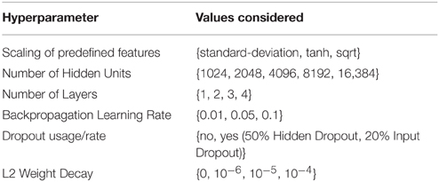
Table 2. Hyperparameters considered for the neural networks.

2.2.5. GPU Implementation

Graphics Processor Units (GPUs) have become essential tools for Deep Learning, because the many layers and units of a DNN give rise to a massive computational load, especially regarding CPU performance. Only through the recent advent of fast accelerated hardware such as GPUs has training a DNN model become feasible (Schmidhuber, 2015). As described in Section 2.2.1, the main equations of a neural net can be written in terms of matrix/vector operations, which are prime candidates for execution on massively parallel hardware architectures. Using state-of-the-art GPU hardware speeds up the training process by several orders of magnitude compared to using an optimized multi-core CPU implementation (Raina et al., 2009). Hence, we implemented the DNNs using the CUDA parallel computing platform and employed NVIDIA Tesla K40 GPUs to achieve speed-ups of 20–100x compared to CPU implementations (see Supplementary Section 5 for an overview on the computational resources that were used).

2.3. The Deeptox Pipeline

As mentioned above, we developed a pipeline, which enables the usage of DNNs for toxicity prediction. The pipeline receives raw training data and supplies predictions for new data. In detail “DeepTox” consists of: (1) cleaning and quality control of the data containing the chemical description of the compounds (Section 2.3.1), (2) creating chemical descriptors as input features for the models (Section 2.3.2), (3) model selection including feature selection if required by the model class (Section 2.3.3), (4) evaluating the quality of models in order to choose the best ones (Section 2.3.4), and (5) combining models to ensemble predictors (Section 2.3.5). The individual steps of the pipeline are visualized as boxes in Figure 6.

FIGURE 6

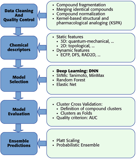
Figure 6. DeepTox pipeline for toxicity prediction.

2.3.1. Data Cleaning and Quality Control

In the first step, DeepTox improves the quality of the training data. We had observed that the chemical substances in question are often mixtures of distinct chemical structures that are not connected by covalent bonds. Therefore, we introduced a fragmentation step to the DeepTox pipeline. In this step, these distinct structures are split into individual “compound fragments.” Examples of frequently recurring compound fragments are Na⁺ and Cl⁻ ions. Upon fragmentation, identical compound fragments can appear multiple times, which are merged by DeepTox. In this merging step, DeepTox semi-automatically labels merged compound fragments, removing contradictory and keeping agreeing measurements. Compound fragments that appear in multiple mixtures can have varying toxicity measurements since Tox21 testing was based on mixtures. If all measurements agree, the fragments are automatically labelled. For disagreeing measurements, an operator has to disentangle the contradictory measurements by assigning activities to compounds in the mixture. If this is impossible, the label is marked to be unknown. All fragments are then normalized by making “H”-atoms explicit and representing aromatic bonds/tautomers consistently, by calculating a canonical formula (Thalheim et al., 2010) using the software Chemaxon. After merging and normalization, the size of the dataset might be reduced. In the case of the Tox21 challenge dataset, 12,707 compounds were reduced to 8694 distinct fragments. To counteract the reduction in the training set size, an optional augmentation step was introduced to DeepTox: kernel-based structural and pharmacological analoging (KSPA), which has been very successful in toxicogenetics (Eduati et al., 2015). The central idea of KSPA is that public databases already contain toxicity assays that are similar to the assay under investigation. KSPA identifies these similar assays by high correlation values and adds their compounds and measurements to the given dataset. Thus, the dataset is enriched with both similar structures and similar assays from public data (see Supplementary Section 2). This typically leads to a performance improvement of Deep Learning methods due to increased datasets. Overall, the data cleaning and quality control procedure improves the predictive performance of the DNNs.

2.3.2. Chemical Descriptors

For Deep Learning, a large number of correlated features is favorable to achieve high performance (see Sections 1 and Krizhevsky et al., 2012). Hence, DeepTox calculates as many types of features as possible, which can be grouped into two basic categories: static and dynamic features. Static features are typically identified by experts as promising properties for predicting biological activity or toxicity. Examples are atom counts, surface areas, and the presence or absence of a predefined substructure in a compound. Since static features are defined a priori, the number of static features that represent a molecule is fixed. For the static features, DeepTox calculates a number of numerical features based on the topological and physical properties of each compound using off-the-shelf software (Cao et al., 2013). These static features include weight, Van der Waals volume, and partial charge information. DeepTox also calculates the presence and absence of 2500 predefined toxicophore features, i.e., patterns of substructures previously reported as toxicophores in the literature (e.g., Kazius et al., 2005), and standard binary and count features such as MACCS and PCFP. Dynamic features are extracted on the fly from the chemical structure of a compound in a prespecified way (e.g., ECFP fingerprint features, Rogers and Hahn, 2010) The DeepTox pipeline uses JCompoundMapper (Hinselmann et al., 2011) to create dynamic features. Dynamic features are often highly specific and therefore sparse. Even if a huge (possibly infinite) number of different dynamic features exists, handling the dataset would remain feasible, as absent features are not reported. Normally, either the presence of a feature (binary) or the count of a feature (discrete) is reported for each compound. While many of these sparse features may be uninformative, some dynamic features may be specific to toxic effects.

The DeepTox pipeline uses a large number of different types of static or dynamic features (see Supplementary Section 1). Different types of input features have substantially different scales and distributions which poses a problem for DNNs. To make all of them available in the same range, DeepTox both standardizes real-valued and count features and applies the tanh nonlinearity. If the software libraries fail to compute a particular feature, median-imputation is performed to substitute the missing value before standardization. The Tox21 dataset in particular comprised several thousands of static features and hundreds of millions of dynamic features that were sparsely coded.

2.3.3. Deeptox Model Selection and Complementary Models

Model Selection is the key step in the DeepTox pipeline. Its goal is to find a model that describes the training data (i.e., assay measurements of compounds) well and can be used to predict assay outcomes of unmeasured compounds.

The main workhorses in the model building part of the DeepTox pipeline are Deep Neural Networks (DNNs), which are described above. Here, we present complementary learning techniques that are included in the DeepTox model building part. These techniques include SVMs, random forests (RF), and elastic nets. These methods are used for cross-checking, supplementing the Deep Learning models, and for ensemble learning to complement DNNs. DeepTox considers both similarity-based method, such as SVMs, and feature-based methods, such as random random forests and elastic nets.

2.3.3.1. Support vector machines

SVMs are large-margin classifiers that are based on the concept of structural risk minimization. They are widely used in chemoinformatics (Mohr et al., 2010; Rosenbaum et al., 2011). SVMs are similarity-based machine learning methods and therefore depend on a kernel function that determines the similarity of two compounds.

The choice of similarity measure is crucial to the performance of SVMs. DeepTox uses a linear kernel as a similarity measure between two compounds x and z, and variations of the Tanimoto kernel:

• $K_{\text{linear}}(x,z)={\displaystyle {\sum }_{p\in {P}}N(p,x)·N(p,z)}$,

• $K_{\text{Minmax}}(x,z)=\frac{{\displaystyle {\sum }_{p\in {P}}\min }N(p,x),N(p,z)}{{\displaystyle {\sum }_{p\in {P}}\max }N(p,x),N(p,z)}$,

• $K_{\text{Minmax}\_\text{new}}(x,z)=\frac{{\displaystyle {\sum }_{p\in {P}N(p,x)+N(p,z)>0}\frac{\min (N(p,x),N(p,z))}{\max (N(p,x),N(p,z))}}}{{\displaystyle {\sum }_{p\in {P}N(p,x)+N(p,z)>0}1}}$,

where N(p, x) quantifies feature p for compound x, and ${P}$ features are considered for a set of compounds. For binary input features, N(p, x) indicates whether a substructure p occurs in the molecule x. For integer-valued input features, N(p, x) is the standardized occurrence count of p in x. For real-valued input features, N(p, x) is the standardized value of a feature p for molecule x.

Our novel MinMax kernel K_{Minmax_new}(x, z) allows continuous features (e.g., partial charges) to be combined with with discrete (e.g., atom counts) and binary (e.g., substructure indicators) features. Since only positive values are allowed, DeepTox splits continuous and count features into positive and negative parts after centering them by the mean or the median.

The hyperparameters for learning SVM models are the SVM regularization parameter, a shrinkage/growth parameter for the kernel similarity, and weights of kernel matrices. Hyperparameters were selected as for DNNs.

2.3.3.2. Random forests

Random forest (Breiman, 2001) approaches construct decision trees for classification, and average over many decision trees for the final classification. Each individual tree uses only a subset of samples and a subset of features, both chosen randomly. In order to construct decision trees, features that optimally separate the classes must be chosen at each node of the tree. Optimal features can be selected based on the information gain criterion or the Gini coefficient. The hyperparameters for random forests are the number of trees, the number of features considered in each step, the number of samples, the feature choice, and the feature type. Random forests require a preprocessing step that reduces the number of features. The t-test and Fisher's exact test were used for real-valued and binary features, respectively.

2.3.3.3. Elastic net

Elastic nets (Friedman et al., 2010; Simon et al., 2011) learn linear regression functions. They basically compute least-square solutions. However, in contrast to ordinary least squares the objective includes a penalty term—a weighted combination between the pure L1 and the pure L2 norm on the coefficients of the linear function. The L1 and L2 regularization leads to sparse solutions via the L1 term and to solutions without large coefficients via the L2 term. The L1 term selects features, and the L2 term prevents model overfitting due to over-reliance on single features. In the Tox21 challenge DeepTox used only static features for elastic net. Since elastic nets built this way typically showed poorer performance than Deep Learning, SVMs and random forests, they were rarely included in the ensembles of the Tox21 challenge.

2.3.4. Model Evaluation

DeepTox determines the performance of our methods by cluster cross-validation. In contrast to standard cross-validation, in which the compounds are distributed randomly across cross-validation folds, clusters of compounds are distributed. Concretely, we used Tanimoto similarity based on ECFP4 fingerprints and single linkage clustering to identify compound clusters. A similarity threshold of 0.7 gave us many small clusters that we then distributed randomly across the folds. DeepTox considers two aspects for defining the cross-validation folds: the ratio of actives to inactives and the similarity of compounds.

The ratio of actives to inactives in the cross-validation folds should be close to the ratio expected in future data. In the Tox21 challenge training dataset, a certain number of compounds were measured in only a few assays, whereas we expected the compounds in the final test set to be measured in all twelve assays. Therefore, in the cross-validation folds, only compounds with labels from at least eight of the twelve assays were included. Thus, we ensured that the ratios of actives to inactives in the cross-validation folds were similar to that in the final test data.

The compounds in different cross-validation folds should not be overly similar. A compound in the test fold that is similar to a compound in the training folds could easily be classified correctly by all methods simply based on the overall similarity. In this case, information about the performance of the methods is lost. To avoid that excessively similar compounds are in the test and in the training fold during model evaluation, DeepTox performs cluster cross-validation, which guarantees a minimum distance between compounds of all folds (even across all clusters) if single-linkage clustering is performed. In the challenge, the clusters that resulted from single-linkage clustering of the compounds were distributed among five cross-validation folds. The similarity measure for clustering was the chemical similarity given by ECFP4 fingerprints. In cluster cross-validation, cross-validation folds contain structurally similar compounds that often share the same scaffold or large substructures.

For the Tox21 challenge, the compounds of the leaderboard set were considered to be an additional cross-validation fold. Aside from computing a mean performance over the cross-validation folds, DeepTox also considered the performance on the leaderboard fold as an additional criterion for performance comparisons.

2.3.5. Ensembles of Models

DeepTox constructs ensembles that contain DNNs and complementary models. For the ensembles, the DeepTox pipeline gives high priority to DNNs, as they tend to perform better than other methods. The pipeline selects ensemble members based on their cross-validation performance and, for the Tox21 challenge dataset, their performance on the leaderboard set. DeepTox uses a variety of criteria to choose the methods that form the ensembles, which led to the different final predictions in the challenge. These criteria were the cross-validation performances and the performance on the leader board set, as well as independence of the methods. The performance criteria ensure that very high-performing models form the ensembles, while the independence criterion ensures that ensembles consist of models built by different methods, or that ensembles are built from different sets of features.

A problem that arises when building ensembles is that values predicted by different models are on different scales. To make the predictions comparable, DeepTox employs Platt scaling (Platt, 1999) to transform them into probabilistic predictions. Platt scaling uses a separate cross-validation run to supply probabilities. Note that probabilities predicted by models such as logistic regression are not trustworthy as they can overfit to the training set. Therefore, a separate run with predictions on unseen data must be performed to calibrate the predictions of a model in such a way that they are trustworthy probabilities. Since the arithmetic mean is not a reasonable choice for combining the predictions of different models, DeepTox uses a probabilistic approach with similar assumptions as naive Bayes (see Supplementary Section 3) to fully exploit the probabilistic predictions in our ensembles.

3. Results

3.1. Benefit of Multi-Task Learning

We were able to apply multi-task learning in the Tox21 challenge because most of the compounds were labeled for several tasks (see Section 1). Multi-task learning has been shown to enhance the performance of DNNs when predicting biological activities at the protein level (Dahl et al., 2014). Since the twelve different tasks of the Tox21 challenge data were highly correlated, we implemented multi-task learning in the DeepTox pipeline.

To investigate whether multi-task learning improves the performance, we compared single-task and multi-task neural networks on the Tox21 leaderboard set. Furthermore, we computed an SVM baseline (linear kernel). Table 3 lists the resulting AUC values and indicates the best result for each task in italic font. The results for DNNs are the means over 5 networks with different random initializations. Both multi-task and single-task networks failed on an assay with a very unbalanced class distribution. For this assay, the data contained only 3 positive examples in the leaderboard set. For 10 out of 12 assays, multi-task networks outperformed single-task networks.

TABLE 3

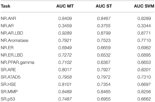
Table 3. Comparison: multi-task (MT) with single-task (ST) learning and SVM baseline evaluated on the leaderboard-set.

3.2. Learning of Toxicophore Representations

As mentioned in Section 1, neurons in different hidden layers of the network may encode toxicophore features. To check whether Deep Learning does indeed construct toxicophores, we performed separate experiments. In the challenge models, toxicophores (see Section 2.3.2) were used as input features. We removed these features to withhold all toxicophore-related substructures from the network input, and were thus able to check whether toxicophores were constructed automatically by DNNs.

We trained a multi-task deep network on the Tox21 data using exclusively ECFP4 fingerprint features, which had similar performance as a DNN trained on the full descriptor set (see Supplementary Section 4, Supplementary Table 1). ECFP fingerprint features encode substructures around each atom in a compound up to a certain radius. Each ECFP fingerprint feature counts how many times a specific substructure appears in a compound. After training, we looked for possible associations between all neurons of the networks and 1429 toxicophores, that were available as described in Section 2.3.2. We checked the associations using a U-test, in which a neuron was characterized by its activation over the compounds of the training set and a toxicophore was characterized by its presence/absence in the training set compounds. The alternative hypothesis for the test was that compounds containing the toxicophore substructure have different activations than compounds that do not contain the toxicophore substructure. Bonferroni multiple testing correction was applied afterwards, that is the p-values from the U-test were multiplied by the number of hypothesis, concretely the number of toxicophores (1429) times the number of neurons of the network (16,384). After this correction, 99% of neurons in the first hidden layer had a significant association with at least one toxicophore feature using a significance threshold of 0.05. The number of neurons with significant associations decreases with increasing level of the layer. In the second layer, there are 97% neurons with a significant association and 90 and 87% in the third and fourth layer, respectively (see Figure 7A). Next we investigated the correlation of known toxicophores to neurons in different layers to quantify their matching. To this end, we used the rank-biserial correlation which is compatible to the previously used U-test. To limit false detections, we constrained the analysis to estimates with a variance < 0.01. We observed that higher layers have a higher number of neurons with rank-biserial correlation above 0.6 (see Figure 7B). This means features in higher layers match toxicophores more precisely.

FIGURE 7

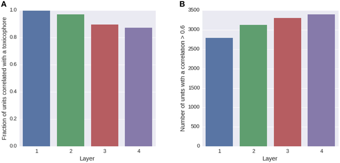
Figure 7. Quantity of neurons with significant associations to toxicophores. (A) The histogram shows the fraction of neurons in a layer that yield significant correlations to a toxicophore. With an increasing level of the layer, the number of neurons with significant correlation decreases. (B) The histogram shows the number of neurons in a layer that exceed a correlation threshold of 0.6 to their best correlated toxicophore. Contrary to (A) the number of neurons increases with the network layer. Note that each layer consisted of the same number of neurons.

The decrease in the number of neurons with significant associations with toxicophores through the layers and the simultaneous increase of neurons with high correlation can be explained by the typical characteristics of a DNN: In lower layers, features code for small substructures of toxicophores, while in higher layers they code for larger substructures or whole toxicophores. Features in lower layers are typically part of several higher layer features, and therefore correlate with more toxicophores than higher level features, which explains the decrease of neurons with significant associations to toxicophores. Features in higher layers are more specific and are therefore correlated more highly with toxicophores, which explains the increase of neurons with high correlation values. Our findings underline that deep networks can indeed learn to build complex toxicophore features with high predictive power for toxicity.

Visual inspection of the results also confirmed that lower layers tended to learn smaller features, often focusing on single functional groups, such as sulfonic acid groups (see row 1 and 2 of Figure 8), while in higher layers the correlations tended to be with larger toxicophore clusters (row 3 of Figure 8). Most importantly, these learned toxicophore structures demonstrated that Deep Learning can support finding new chemical knowledge that is encoded in its hidden units.

FIGURE 8

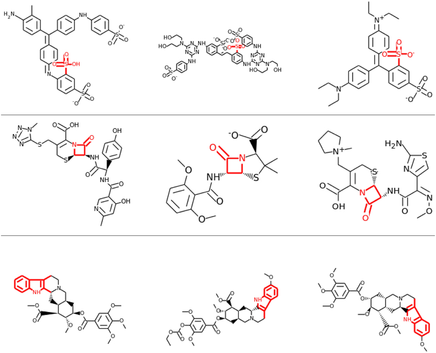
Figure 8. Feature Construction by Deep Learning. Neurons that have learned to detect the presence of toxicophores. Each row shows a particular hidden unit in a learned network that correlates highly with a particular known toxicophore feature. The row shows the three chemical compounds that had the highest activation for that neuron. Indicated in red is the toxicophore structure from the literature that the neuron correlates with. The first row and the second row are from the first hidden layer, the third row is from a higher-level layer.

3.3. Comparison of DNN and Complementary Methods

We selected the best-performing models from each method in the DeepTox pipeline based on an evaluation of the DeepTox cross-validation sets and evaluated them on the final test set. The methods we compared were DNNs, SVMs (Tanimoto kernel), random forests (RF), and elastic net (ElNet). Table 4 shows the AUC values for each method and each dataset. We also provided the mean AUC over the NR and SR panel, and the mean AUC over all datasets. The results confirm the superiority of Deep Learning over complementary methods for toxicity prediction by outperforming other approaches in 10 out of 15 cases.

TABLE 4

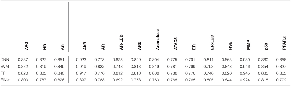
Table 4. AUC Results for different learning methods as part of DeepTox evaluated on the final test set.

3.4. Tox21 Data Challenge Results

The DeepTox pipeline, which is dominated by DNNs, consistently showed very high performance compared to all competing methods. It won a total of 9 of the 15 challenges and did not rank lower than fifth place in any of the subchallenges In particular, it achieved the best average AUC in both the SR and the NR panel, and additionally the best average AUC across the whole set of sub-challenges. It was thus declared winner of the Nuclear Receptor and the Stress Response panel, as well as the overall Tox21 Grand Challenge.

The leading teams' results (team names abbreviated) from all 12 subchallenges and the average results over the 12 subchallenges and the subchallenges that were part of the “Nuclear Receptor” and the “Stress Response” panel, respectively, are given in Table 5. The best results are indicated in bold with gray background, the second-best results with light gray background.

TABLE 5

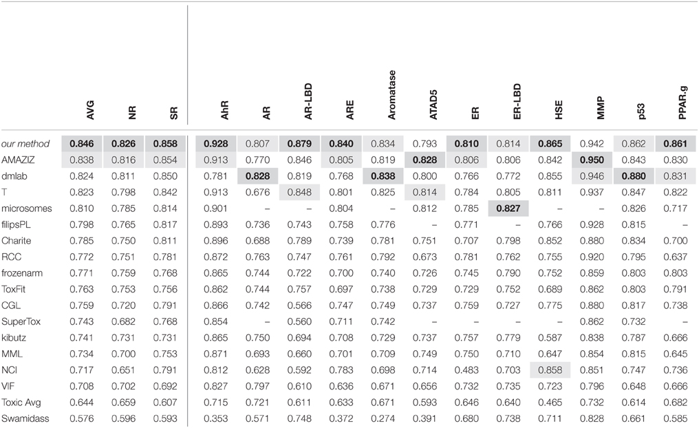
Table 5. The leading teams' AUC Results on the final test set in the Tox21 challenge.

The Tox21 challenge result can be summarized as follows: The Deep-Learning-based DeepTox pipeline clearly outperformed all competitors.

4. Discussion

In this paper, we have introduced the DeepTox pipeline for toxicity prediction based on Deep Learning.

Deep Learning is known to learn abstract representations of the input data with higher levels of abstractions in higher layers (LeCun et al., 2015). This concept has been relatively straightforward to demonstrate in image recognition, where simple objects, such as edges and simple blobs, in lower layers are combined to abstract objects in higher layers (Lee et al., 2009). In toxicology, however, it was not known how the data representations from Deep Learning could be interpreted. We could show that many hidden neurons represent previously known toxicophores (Kazius et al., 2005)—proven concepts which have formerly been handcrafted over decades by experts in the field. Naturally, we conclude that these representations also include novel, previously undiscovered toxicophores that are latent in the data. Using these representations, our pipeline outperformed methods that were specifically tailored to toxicological applications.

Successful deep learning is facilitated by Big Data and the use of graphical processing units (GPUs). In this case, Big Data is a blessing rather than a curse. However, Big Data implies a large computational demand. GPUs alleviate the problem of large computation times, typically by using CUDA kernels on Nvidia cards (Raina et al., 2009; Unterthiner et al., 2014, 2015; Clevert et al., 2015). Concretely, training a single DNN on the Tox21 dataset takes about 10 min on an Nvidia Tesla K40 with our optimized implementation. However, we had to train thousands of networks in order to investigate different hyperparameter settings via our cross-validation procedure, which is crucial for the performance of DNNs. The hyperparameter search was parallelized across multiple GPUs. Concluding, we consider the use of GPUs a necessity and recommend the use of multiple GPU units.

Similar to the successes in other fields (Dahl et al., 2012; Krizhevsky et al., 2012; Deng et al., 2013; Graves et al., 2013; Socher and Manning, 2013; Baldi et al., 2014; Sutskever et al., 2014), Deep Learning has increased the predictive performance of computational methods in toxicology. As confirmed by the NIH¹, the high quality of the models in the Tox21 challenge makes them suitable for deployment in leading-edge toxicological research. We believe that Deep Learning is highly suited to predicting toxicity and is capable of significantly influencing this field in the future.

Funding

The research was funded by ChemBioBridge and MrSymBioMath.

Conflict of Interest Statement

The authors declare that the research was conducted in the absence of any commercial or financial relationships that could be construed as a potential conflict of interest.

Acknowledgments

We thank ChemAxon² for providing an academic license: Chem Base was used for structure searching and chemical database access and management and Standardizer was used for structure canonicalization and transformation, JChem 14.9.1.0, 2014. Further we thank Honglak Lee for the permission to use his images and the NVIDIA corporation for the GPU donations which made this research possible.

Supplementary Material

The Supplementary Material for this article can be found online at: https://www.frontiersin.org/article/10.3389/fenvs.2015.00080

Footnotes

1. ^https://ncats.nih.gov/news/releases/2015/tox21-challenge-2014-winners.

2. ^https://www.chemaxon.com

References

Ajmani, S., Jadhav, K., and Kulkarni, S. A. (2006). Three-dimensional QSAR using the k-nearest neighbor method and its interpretation. J. Chem. Inf. Model. 46, 24–31. doi: 10.1021/ci0501286

PubMed Abstract | CrossRef Full Text | Google Scholar

Andersen, M. E., and Krewski, D. (2009). Toxicity testing in the 21st century: bringing the vision to life. Toxicol. Sci. 107, 324–330. doi: 10.1093/toxsci/kfn255

PubMed Abstract | CrossRef Full Text | Google Scholar

Baldi, P., Sadowski, P., and Whiteson, D. (2014). Searching for exotic particles in high-energy physics with deep learning. Nat. Commun. 5:4308. doi: 10.1038/ncomms5308

PubMed Abstract | CrossRef Full Text | Google Scholar

Bartkova, J., Hořejší, Z., Koed, K., Krämer, A., Tort, F., Zieger, K., et al. (2005). DNA damage response as a candidate anti-cancer barrier in early human tumorigenesis. Nature 434, 864–870. doi: 10.1038/nature03482

PubMed Abstract | CrossRef Full Text | Google Scholar

Bender, A., Mussa, H., Glen, R. C., and Reiling, S. (2004). Molecular similarity searching using atom environments, information-based feature selection, and a naive Bayesian classifier. J. Chem. Inf. Comput. Sci. 44, 170–178. doi: 10.1021/ci034207y

PubMed Abstract | CrossRef Full Text | Google Scholar

Bottou, L. (2010). “Large-scale machine learning with stochastic gradient descent,” in Proceedings of the 19th International Conference on Computational Statistics (COMPSTAT 2010), eds Y. Lechevallier and G. Saporta (Paris), 177–187. doi: 10.1007/978-3-7908-2604-3_16

PubMed Abstract | CrossRef Full Text

Breiman, L. (2001). Random forests. Mach. Learn. 45, 5–32. doi: 10.1023/A:1010933404324

CrossRef Full Text | Google Scholar

Cao, D.-S., Huang, J.-H., Yan, J., Zhang, L.-X., Hu, Q.-N., Xu, Q.-S., et al. (2012). Kernel k-nearest neighbor algorithm as a flexible SAR modeling tool. Chemometr. Intell. Lab. 114, 19–23. doi: 10.1016/j.chemolab.2012.01.008

CrossRef Full Text | Google Scholar

Cao, D.-S., Xu, Q.-S., Hu, Q.-N., and Liang, Y.-Z. (2013). ChemoPy: freely available python package for computational biology and chemoinformatics. Bioinformatics 29, 1092–1094. doi: 10.1093/bioinformatics/btt105

PubMed Abstract | CrossRef Full Text | Google Scholar

Caruana, R. (1997). Multitask learning. Mach. Learn. 28, 41–75. doi: 10.1023/A:1007379606734

PubMed Abstract | CrossRef Full Text | Google Scholar

Chawla, A., Repa, J. J., Evans, R. M., and Mangelsdorf, D. J. (2001). Nuclear receptors and lipid physiology: opening the X-files. Science 294, 1866–1870. doi: 10.1126/science.294.5548.1866

PubMed Abstract | CrossRef Full Text | Google Scholar

Cireşan, D. C., Meier, U., and Schmidhuber, J. (2012a). “Multi-column deep neural networks for image classification,” in Proceedings of the 2012 IEEE Conference on Computer Vision and Pattern Recognition (CVPR) (Providence, RI), 3642–3649. doi: 10.1109/CVPR.2012.6248110

CrossRef Full Text | Google Scholar

Cireşan, D. C., Giusti, A., Gambardella, L. M., and Schmidhuber, J. (2013). “Mitosis detection in breast cancer histology images with deep neural networks,” in 16th International Conference on Medical Image Computing and Computer-Assisted Intervention (MICCAI 2013), eds K. Mori, I. Sakuma, Y. Sato, C. Barillot, and N. Navab (Nagoya), 411–418. doi: 10.1007/978-3-642-40763-5_51

CrossRef Full Text | Google Scholar

Cireşan, D. C., Meier, U., Gambardella, L. M., and Schmidhuber, J. (2012b). “Deep big multilayer perceptrons for digit recognition,” in Neural Networks: Tricks of the Trade, eds G. Montavon, G. B. Orr, and K.-R. Müller (Heidelberg: Springer), 581–598.

Clevert, D.-A., Mayr, A., Unterthiner, T., and Hochreiter, S. (2015). “Rectified factor networks,” in Advances in Neural Information Processing Systems 28 (NIPS 2015), eds C. Cortes, N. Lawrence, D. Lee, M. Sugiyama, and R. Garnett (Montreal, QC), 1846–1854.

Google Scholar

Dahl, G. E., Jaitly, N., and Salakhutdinov, R. R. (2014). Multi-task neural networks for QSAR predictions. arXiv:1406.1231.

Google Scholar

Dahl, G. E., Yu, D., Deng, L., and Acero, A. (2012). Context-dependent pre-trained deep neural networks for large vocabulary speech recognition. IEEE T Audio Speech 20, 30–42. doi: 10.1109/TASL.2011.2134090

CrossRef Full Text | Google Scholar

Darnag, R., Mazouz, E. M., Schmitzer, A., Villemin, D., Jarid, A., and Cherqaoui, D. (2010). Support vector machines: development of QSAR models for predicting anti-HIV-1 activity of TIBO derivatives. Eur. J. Med. Chem. 28, 1075–1086. doi: 10.1016/j.ejmech.2010.01.002

PubMed Abstract | CrossRef Full Text | Google Scholar

Deng, L., Hinton, G. E., and Kingsbury, B. (2013). “New types of deep neural network learning for speech recognition and related applications: an overview,” in Proceedings of the 2013 IEEE International Conference on Acoustics, Speech and Signal Processing (ICASSP) (Vancouver, BC), 8599–8603. doi: 10.1109/ICASSP.2013.6639344

CrossRef Full Text

Eduati, F., Mangravite, L. M., Wang, T., Tang, H., Bare, J. C., Huang, R., et al. (2015). Prediction of human population responses to toxic compounds by a collaborative competition. Nat. Biotechnol. 33, 933–940. doi: 10.1038/nbt.3299

PubMed Abstract | CrossRef Full Text | Google Scholar

Friedman, J., Hastie, T., and Tibshirani, R. (2010). Regularization paths for generalized linear models via coordinate descent. J. Stat. Softw. 33, 1–22. doi: 10.18637/jss.v033.i01

PubMed Abstract | CrossRef Full Text | Google Scholar

Glorot, X., Bordes, A., and Bengio, Y. (2011). “Deep sparse rectifier neural networks,” in Fourteenth International Conference on Artificial Intelligence and Statistics (AISTATS 2011), eds G. J. Gordon, D. B. Dunson, and M. Dudík (Fort Lauderdale, FL), 315–323.

Graves, A., Mohamed, A. R., and Hinton, G. E. (2013). “Speech recognition with deep recurrent neural networks,” in Proceedings of the 2013 IEEE International Conference on Acoustics, Speech and Signal Processing (ICASSP) (Vancouver, BC), 6645–6649. doi: 10.1109/ICASSP.2013.6638947

CrossRef Full Text

Grün, F., and Blumberg, B. (2007). Perturbed nuclear receptor signaling by environmental obesogens as emerging factors in the obesity crisis. Rev. Endocr. Metab. Dis. 8, 161–171. doi: 10.1007/s11154-007-9049-x

PubMed Abstract | CrossRef Full Text | Google Scholar

Hinselmann, G., Rosenbaum, L., Jahn, A., Fechner, N., and Zell, A. (2011). jCompoundMapper: an open source Java library and command-line tool for chemical fingerprints. J. Cheminform. 3:3. doi: 10.1186/1758-2946-3-3

PubMed Abstract | CrossRef Full Text | Google Scholar

Hinton, G. E., Srivastava, N., Krizhevsky, A., Sutskever, I., and Salakhutdinov, R. R. (2012). Improving neural networks by preventing co-adaptation of feature detectors. arXiv:1207.0580.

Google Scholar

Hochreiter, S. (1991). Untersuchungen Zu Dynamischen Neuronalen Netzen. Master's thesis, Institut für Informatik, Lehrstuhl Prof. Dr. Dr. h.c. Brauer, Technische Universität München.

Hochreiter, S., Bengio, Y., Frasconi, P., and Schmidhuber, J. (2000). “Gradient flow in recurrent nets: the difficulty of learning long-term dependencies,” in A Field Guide to Dynamical Recurrent Networks, eds J. Kolen and S. Kremer (New York, NY: IEEE), 237–244.

Google Scholar

Huang, R., Sakamuru, S., Martin, M. T., Reif, D. M., Judson, R. S., Houck, K. A., et al. (2014). Profiling of the Tox21 10K compound library for agonists and antagonists of the estrogen receptor alpha signaling pathway. Sci. Rep. 4:5664. doi: 10.1038/srep05664

PubMed Abstract | CrossRef Full Text | Google Scholar

Jaeschke, H., McGill, M. R., and Ramachandran, A. (2012). Oxidant stress, mitochondria, and cell death mechanisms in drug-induced liver injury: lessons learned from acetaminophen hepatotoxicity. Drug Metab. Rev. 44, 88–106. doi: 10.3109/03602532.2011.602688

PubMed Abstract | CrossRef Full Text | Google Scholar

Kashima, H., Tsuda, K., and Inokuchi, A. (2003). “Marginalized kernels between labeled graphs,” in Proceedings of the Twentieth International Conference on Machine Learning (ICML 2003), eds T. Fawcett and N. Mishra (Washington, DC), 321–328.

Kashima, H., Tsuda, K., and Inokuchi, A. (2004). “Kernels for graphs,” in Kernel Methods in Computational Biology, eds B. Schölkopf, K. Tsuda, and J.-P. Vert (Cambridge, MA: MIT Press), 155–170.

Google Scholar

Kauffman, G. W., and Jurs, P. C. (2001). QSAR and k-nearest neighbor classification analysis of selective cyclooxygenase-2 inhibitors using topologically-based numerical descriptors. J. Chem. Inf. Comput. Sci. 41, 1553–1560. doi: 10.1021/ci010073h

PubMed Abstract | CrossRef Full Text | Google Scholar

Kazius, J., McGuire, R., and Bursi, R. (2005). Derivation and validation of toxicophores for mutagenicity prediction. J. Med. Chem. 48, 312–320. doi: 10.1021/jm040835a

PubMed Abstract | CrossRef Full Text | Google Scholar

Klambauer, G., Wischenbart, M., Mahr, M., Unterthiner, T., Mayr, A., and Hochreiter, S. (2015). Rchemcpp: a web service for structural analoging in ChEMBL, Drugbank and the Connectivity Map. Bioinformatics 31, 3392–3394. doi: 10.1093/bioinformatics/btv373

PubMed Abstract | CrossRef Full Text | Google Scholar

Krewski, D., Acosta, D. Jr, Andersen, M., Anderson, H., Bailar III, J. C., Boekelheide, K., et al. (2010). Toxicity testing in the 21st century: a vision and a strategy. J. Toxicol. Environ. Health 13, 51–138. doi: 10.1080/10937404.2010.483176

PubMed Abstract | CrossRef Full Text | Google Scholar

Krizhevsky, A., Sutskever, I., and Hinton, G. E. (2012). “ImageNet classification with deep convolutional neural networks,” in Advances in Neural Information Processing Systems 25 (NIPS 2012), eds F. Pereira, C. Burges, L. Bottou, and K. Weinberger (Lake Tahoe), 1097–1105.

Labbe, G., Pessayre, D., and Fromenty, B. (2008). Drug-induced liver injury through mitochondrial dysfunction: mechanisms and detection during preclinical safety studies. Fund. Clin. Pharmacol. 22, 335–353. doi: 10.1111/j.1472-8206.2008.00608.x

PubMed Abstract | CrossRef Full Text | Google Scholar

LeCun, Y., Bengio, Y., and Hinton, G. E. (2015). Deep learning. Nature 521, 436–444. doi: 10.1038/nature14539

PubMed Abstract | CrossRef Full Text | Google Scholar

Lee, H., Grosse, R., Ranganath, R., and Ng, A. Y. (2011). Unsupervised learning of hierarchical representations with convolutional deep belief networks. Commun. ACM 54, 95–103. doi: 10.1145/2001269.2001295

CrossRef Full Text | Google Scholar

Lee, H., Grosse, R., Ranganath, R., and Ng, A. Y. (2009). “Convolutional deep belief networks for scalable unsupervised learning of hierarchical representations,” in Proceedings of the 26th International Conference on Machine Learning (ICML 2009), eds A. P. Danyluk, L. Bottou, and M. L. Littman (Montreal, QC), 609–616. doi: 10.1145/1553374.1553453

CrossRef Full Text

Luco, J. M., and Ferretti, F. H. (1997). QSAR based on multiple linear regression and PLS methods for the anti-HIV activity of a large group of HEPT derivatives. J. Chem. Inf. Comput. Sci. 37, 392–401. doi: 10.1021/ci960487o

PubMed Abstract | CrossRef Full Text | Google Scholar

Ma, J., Sheridan, R. P., Liaw, A., Dahl, G. E., and Svetnik, V. (2015). Deep neural nets as a method for quantitative Structure-Activity relationships. J. Chem. Inf. Model. 55, 263–274. doi: 10.1021/ci500747n

PubMed Abstract | CrossRef Full Text | Google Scholar

Mahé, P., Ralaivola, L., Stoven, V., and Vert, J.-P. (2006). The pharmacophore kernel for virtual screening with support vector machines. J. Chem. Inf. Model. 46, 2003–2014. doi: 10.1021/ci060138m

PubMed Abstract | CrossRef Full Text | Google Scholar

Mahé, P., Ueda, N., Akutsu, T., Perret, J.-L., and Vert, J.-P. (2005). Graph kernels for molecular Structure-Activity relationship analysis with support vector machines. J. Chem. Inf. Model. 45, 939–951. doi: 10.1021/ci050039t

PubMed Abstract | CrossRef Full Text | Google Scholar

Mohr, J. A., Jain, B. J., and Obermayer, K. (2008). Molecule kernels: a descriptor- and alignment-free quantitative Structure-Activity relationship approach. J. Chem. Inf. Model. 48, 1868–1881. doi: 10.1021/ci800144y

PubMed Abstract | CrossRef Full Text | Google Scholar

Mohr, J. A., Jain, B. J., Sutter, A., Laak, A. T., Steger-Hartmann, T., Heinrich, N., et al. (2010). A maximum common subgraph kernel method for predicting the chromosome aberration test. J. Chem. Inf. Model. 50, 1821–1838. doi: 10.1021/ci900367j

PubMed Abstract | CrossRef Full Text | Google Scholar

Nair, V., and Hinton, G. E. (2010). “Rectified linear units improve restricted boltzmann machines,” in Proceedings of the 27th International Conference on Machine Learning (ICML 2010), eds J. Fürnkranz and T. Joachims (Haifa), 807–814.

Ngiam, J., Coates, A., Lahiri, A., Prochnow, B., Le, Q. V., and Ng, A. Y. (2011). “On optimization methods for deep learning,” in Proceedings of the 28th International Conference on Machine Learning (ICML 2011), eds L. Getoor and T. Scheffer (Bellevue, WA), 689–696.

Niu, B., Lu, W.-C., Yang, S.-S., Cai, Y.-D., and Li, G.-Z. (2007). Support vector machine for SAR/QSAR of phenethyl-amines1. Acta Pharma. Sinica. 28, 1075–1086. doi: 10.1111/j.1745-7254.2007.00573.x

PubMed Abstract | CrossRef Full Text | Google Scholar

Platt, J. C. (1999). “Probabilistic outputs for support vector machines and comparisons to regularized likelihood methods,” in Advances in Large Margin Classifiers, eds A. J. Smola, P. Bartlett, B. Schölkopf, and D. Schuurmans (Cambridge, MA: MIT Press), 61–74.

Polishchuk, P. G., Muratov, E. N., Artemenko, A. G., Kolumbin, O. G., Muratov, N. N., and Kuzmin, V. E. (2009). Application of random forest approach to QSAR prediction of aquatic toxicity. J. Chem. Inf. Model. 49, 2481–2488. doi: 10.1021/ci900203n

PubMed Abstract | CrossRef Full Text | Google Scholar

Raina, R., Madhavan, A., and Ng, A. Y. (2009). “Large-scale deep unsupervised learning using graphics processors,” in Proceedings of the 26th International Conference on Machine Learning (ICML 2009), eds A. P. Danyluk, L. Bottou, and M. L. Littman (Montreal, QC), 873–880. doi: 10.1145/1553374.1553486

CrossRef Full Text

Ralaivola, L., Swamidass, S. J., Saigo, H., and Baldi, P. (2005). Graph kernels for chemical informatics. Neural Netw. 18, 1093–1110. doi: 10.1016/j.neunet.2005.07.009

PubMed Abstract | CrossRef Full Text | Google Scholar

Ranzato, M., Boureau, Y.-I., and LeCun, Y. (2008). “Sparse feature learning for deep belief networks,” in Advances in Neural Information Processing Systems 21 (NIPS 2008), eds D. Koller, D. Schuurmans, Y. Bengio, and L. Bottou (Vancouver, BC), 1185–1192.

Rogers, D., and Hahn, M. (2010). Extended-connectivity fingerprints. J. Chem. Inf. Model. 50, 742–754. doi: 10.1021/ci100050t

PubMed Abstract | CrossRef Full Text | Google Scholar

Rosenbaum, L., Hinselmann, G., Jahn, A., and Zell, A. (2011). Interpreting linear support vector machine models with heat map molecule coloring. J. Cheminform. 3:11. doi: 10.1186/1758-2946-3-11

PubMed Abstract | CrossRef Full Text | Google Scholar

Rumelhart, D. E., Hinton, G. E., and Williams, R. J. (1986). Learning representations by back-propagating errors. Nature 323, 533–536. doi: 10.1038/323533a0

CrossRef Full Text

Rusyn, I., and Daston, G. P. (2010). Computational toxicology: realizing the promise of the toxicity testing in the 21st century. Environ. Health Perspect. 118, 1047–1050. doi: 10.1289/ehp.1001925

PubMed Abstract | CrossRef Full Text | Google Scholar

Sagardia, I., Roa-Ureta, R. H., and Bald, C. (2013). A new QSAR model, for angiotensin I-converting enzyme inhibitory oligopeptides. Food Chem. 136, 1370–1376. doi: 10.1016/j.foodchem.2012.09.092

PubMed Abstract | CrossRef Full Text | Google Scholar

Schmidhuber, J. (2015). Deep learning in neural networks: an overview. Neural Netw. 61, 85–117. doi: 10.1016/j.neunet.2014.09.003

PubMed Abstract | CrossRef Full Text | Google Scholar

Shukla, S. J., Huang, R., Austin, C. P., and Xia, M. (2010). The future of toxicity testing: a focus on in vitro methods using a quantitative high-throughput screening platform. Drug Discov. Today 15, 997–1007. doi: 10.1016/j.drudis.2010.07.007

PubMed Abstract | CrossRef Full Text | Google Scholar

Simon, N., Friedman, J., Hastie, T., and Tibshirani, R. (2011). Regularization paths for Cox's proportional hazards model via coordinate descent. J. Stat. Softw. 39, 1–13. doi: 10.18637/jss.v039.i05

CrossRef Full Text | Google Scholar

Socher, R., and Manning, C. D. (2013). “Deep learning for NLP (without magic),” in 2013 Conference of the North American Chapter of the Association for Computational Linguistics: Human Language Technologies, eds L. Vanderwende, H. D. III, and K. Kirchhoff (Atlanta, GA), 1–3.

Srivastava, N., Hinton, G. E., Krizhevsky, A., Sutskever, I., and Salakhutdinov, R. R. (2014). Dropout: a simple way to prevent neural networks from overfitting. J. Mach. Learn. Res. 15, 1929–1958. doi: 10.1021/ci034160g

CrossRef Full Text | Google Scholar

Sutskever, I., Vinyals, O., and Le, Q. V. (2014). “Sequence to sequence learning with neural networks,” in Advances in Neural Information Processing Systems 27 (NIPS 2014), eds Z. Ghahramani, M. Welling, C. Cortes, N. Lawrence, and K. Weinberger (Montreal, QC), 3104–3112.

Svetnik, V., Liaw, A., Tong, C., Culberson, J., Sheridan, R. P., and Feuston, B. P. (2003). Random forest: a classification and regression tool for compound classification and QSAR modeling. J. Chem. Inf. Comput. Sci. 43, 1947–1958.

PubMed Abstract | Google Scholar

Thalheim, T., Vollmer, A., Ebert, R.-U., Kuhne, R., and Schurmann, G. (2010). Tautomer identification and tautomer structure generation based on the InChI code. J. Chem. Inf. Model. 50, 1223–1232. doi: 10.1021/ci1001179

PubMed Abstract | CrossRef Full Text | Google Scholar

Unterthiner, T., Mayr, A., Klambauer, G., and Hochreiter, S. (2015). Toxicity prediction using deep learning. arXiv:1503.01445.

Google Scholar

Unterthiner, T., Mayr, A., Klambauer, G., Steijaert, M., Ceulemans, H., Wegner, J. K., et al. (2014). “Deep learning as an opportunity in virtual screening,” in NIPS Workshop on Deep Learning and Representation Learning (Montreal, QC).

Verbist, B., Klambauer, G., Vervoort, L., Talloen, W., The QSTAR Consortium, Shkedy, Z., Thas, O., et al. (2015). Using transcriptomics to guide lead optimization in drug discovery projects. Drug Discov. Today 20, 505–513. doi: 10.1016/j.drudis.2014.12.014

PubMed Abstract | CrossRef Full Text | Google Scholar

Vishwanathan, S. V. N., Schraudolph, N. N., Kondor, R., and Borgwardt, K. M. (2010). Graph kernels. J. Mach. Learn. Res. 11, 1201–1242.

PubMed Abstract | Google Scholar

Werbos, P. J. (1974). Beyond Regression: New Tools for Prediction and Analysis in the Behavioral Sciences. Ph.D. thesis, Harvard University.

Xia, X., Maliski, E. G., Gallant, P., and Rogers, D. (2004). Classification of kinase inhibitors using a bayesian model. J. Med. Chem. 47, 4463–4470. doi: 10.1021/jm0303195

PubMed Abstract | CrossRef Full Text | Google Scholar