Quantifying Ecological Constraints on Motion Signaling

Introduction

Animal communication is a particularly interesting area of animal ecology as it underpins the social strategies utilized by animals under a variety of different contexts. Indeed, valuable insights into animal behavior were gained from early descriptions of acoustic signals and the role of color in animal displays. However, it was not until sound spectrographs and spectrophotometers were introduced as tools to quantify these signals that researchers were able to analyze relevant behavior in detail (Kellogg and Stein, 1953; Lythgoe, 1979; Endler, 1990). In addition to facilitating comparisons within and between individuals, these techniques allow for direct comparisons between signals and competing stimuli in the environment. Furthermore, when combined with knowledge of the sensory systems that detect signals, and higher-order brain properties that process further the information collected, researchers are in a position to understand the function and evolution of animal signals.

Environmental influences on signaling are important (Endler, 1992; Lengagne and Slater, 2002; Lohr et al., 2003; Cocroft and Rodriguez, 2005). Of particular note is the interference or masking effect caused by noise in the surrounding habitat (e.g., Fleishman, 1986; Brumm et al., 2004; Brumm and Slabbekoorn, 2005; Witte et al., 2005). In order for a signal to be effective it needs to be detectable by the intended receiver, which means it must be distinguishable from competing environmental noise (Endler, 1992; Fleishman, 1992). In the case of auditory signals, noise can refer to the calls of sympatric species (Greenfield, 1988; Amézquita and Hödl, 2004), anthropogenic sounds (Slabbekoorn and Peet, 2003; Slabbekoorn and Boer-Visser, 2006), rain (Lengagne and Slater, 2002) or even running water (Grafe and Wanger, 2007). Changes in the spectral environment as a consequence of habitat structure, diurnal and seasonal variation in illumination, and meteorological conditions are particularly influential in mediating the detectability of static visual signals, and often influence the spatial distribution of communities and microhabitat selection (Endler and Thery, 1996; Leal and Fleishman, 2002). In the case of visual motion signals, the principal source of noise is the movement of windblown plants (Fleishman, 1988a,b; Peters et al., 2007; Peters, 2008).

Many species use motion-based signals to communicate (Ruibal, 1967; Lorenz, 1971; Purdue and Carpenter, 1972; Hailman and Dzelzkalns, 1974; Ruibal and Philibosian, 1974; Jackson, 1977, 1986; Gibbons, 1979; Fleishman, 1992; How et al., 2007; Ramos and Peters, 2016). A challenge for researchers studying motion-signaling systems is the inherent difficulty of quantifying signals and environmental noise in a meaningful way that facilitates comparisons. While the influence of habitat structure on motion signaling can be inferred by examining the selective use of motor patterns across habitat types (Ramos and Peters, 2016), or prevailing environmental conditions (Ord and Stamps, 2008), it does not directly compare the structure of signal and noise. Environmental effects can also be subtle and difficult to infer from broad scale investigations yet impose considerable constraints on effective signaling that lead signalers to modify display structure (Ord et al., 2007, 2016; Peters et al., 2007). Clearly, to understand in detail the motion signals of animals we need to quantify both the signal and noise in such a way that they are comparable at relevant timescales. This is commonplace for other kinds of signals and we suggest there is growing need to consider in more detail the motion environment in which motion signaling takes place.

The conventional approach to characterize motion-based signals is to create display action patterns to represent simple body movements. These describe changes in position over time, but provide little information on the noise environment or the efficacy of the signal (e.g., Carpenter et al., 1970; Jenssen, 1977). Fleishman (1988a) utilized the first quantitative approach by comparing frequency spectra of the motion patterns from windblown plants to those from lizard displays. Although ground-breaking, these analyses were limited to comparisons of animal motion with single blades of a few different species of grass. Zeil and Zanker (1997) used a two-dimensional elementary motion detection model to describe the properties of motion displays by Fiddler crabs (genus Uca) in terms of signal direction and strength. Subsequently, Peters et al. (2002) applied a gradient detector model to measure the structure of animal signals and whole plants. Furthermore, Peters and Evans (2003) employed the same methodology to compare velocity signatures from lizard signals and plant sequences in order to estimate the relative conspicuousness of each motor pattern in the lizard display. This led to a much better understanding of motion signal structure and opened the path to many studies on the influence of the environment on lizard signaling behavior (Leal and Fleishman, 2004; Ord et al., 2007, 2010; Peters et al., 2007, 2008; Ord and Stamps, 2008; Fleishman and Pallus, 2010).

The use of motion detector algorithms for quantifying animal signals is now the standard way to compare display movements and plant motion noise (Zanker and Zeil, 2005; Fleishman and Pallus, 2010; Pallus et al., 2010). However, all these studies utilize video footage from a single camera view that necessarily assumes the camera is ideally positioned to sample the display. In studies in which environmental noise is also captured from the same camera view and subsequently analyzed (Ord et al., 2007; Fleishman and Pallus, 2010), it is also assumed that the sampled plant motion is sufficient. We suggest that this approach has been informative but restricts our understanding of the context in which motion signals are generated. An analogy from bioacoustics would be the use of a single, highly directional microphone and assuming this reliably samples the noise environment. Indeed, to sample sounds more completely, researchers use omnidirectional microphones (Slabbekoorn and Peet, 2003; Brumm, 2004) or multiple microphones in an array (McGregor et al., 1997; Mennill et al., 2006; Patricelli and Krakauer, 2010).

The efficacy of motion signals will depend very much on microhabitat structure as well as the position of both signaler and receiver (Zeil and Hemmi, 2006; How et al., 2008; Peters, 2010, 2013; Steinberg and Leal, 2013). By way of illustration, Figure 1 represents a hypothetical scene in which a lizard is positioned in the middle of the habitat and surrounded by vegetation that might interfere with the reliable detection of the lizard's display. Importantly, the relevance of surrounding plants, and consequently the noise environment, changes depending on the position of the receiver. A receiver located at viewing position 1 will see plants “a” and “c,” while at viewing position 2, the plant directly occludes the lizard (Figures 1B,C). From viewing position 3, plants “a,” “b,” and “c” are visible and could potentially influence the efficacy of the signal (Figures 1B,C). Another important consideration is the relative distance of the plant from the receiver. As angular speeds (units of speed as perceived from the position of the observer; see Section Digitizing Displays) are distance dependent, the distance between signaler and background plants is predicted to affect differentiation between signal and noise (Peters et al., 2008). This suggests that the masking effect of a plant will change as the receiver moves farther away from the movements, so we would expect quantitative differences between viewing positions 3 and 4.

FIGURE 1

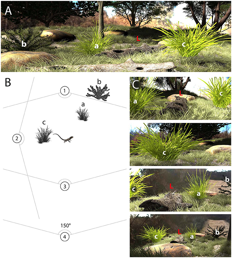
Figure 1. (A) The environment where motion signaling takes place includes plants (a, b, c) that could mask motion-based signals generated by lizards (L). (B) Schematic representation of the scene depicted in (A) showing the lizard and three main plants, as well as four different viewing positions (1–4). (C), The perspective for viewers positioned at each of the four locations differs and serves to illustrate how viewing position will determine the noise environment. Viewing positions 1, 2, and 3 are at a similar distance from the signaler, while 4 is further away. The lizard is completely blocked by plant “c” for a viewer located at viewing position 2 and as such the signal is completely masked by noise. For the other viewing positions, plant “a” is relevant for positions 1, 3, and 4, but its apparent size and masking potential increases when positioned in front of the lizard (viewing position 1) and decreases when behind (viewing position 3, 4). Plant “b” is outside the field of view from viewing position 1, but is relevant from viewing positions 3 and 4. Plant “c” is relevant for viewing positions 1, 3, and 4, and is at the same depth plane as the lizard in each case.

As explained above, the environment in which motion signaling takes place is more complex than we have considered to date. In the present paper we propose a methodology for quantifying the relative performance of motion-based signals in an outdoor field setting. Signals are filmed using two cameras and movements are reconstructed in three dimensions (3D) to ensure the measured structure of signals is not affected by the position of the camera during filming. Motion speeds can then be converted into angular speeds from any user-defined viewing position. Additionally, the habitat where the signals are emitted is mapped in detail for each display, including the position of the lizard relative to the main features of the area. The plants included in the map are filmed under controlled wind conditions to generate environmental noise in a standardized manner. Habitat maps are later used to identify the relevant plants for a given viewing position and distance, and their motion speeds converted to angular speeds. Resultant speed distributions are compared to those obtained from lizard displays in order to consider the extent to which environmental noise might mask the signals of lizards. By repeating this process for other viewing positions and summarizing the results we provide an estimate for the robustness of the signal in that particular habitat. To our knowledge, no one has attempted to quantify both the animal signal and habitat structure in such detail in a field setting.

We illustrate our approach by quantifying the relative contrast of motion-based signals produced by the Australian mallee military dragon Ctenophorus fordi, from two populations featuring distinct habitat characteristics. Importantly, our approach does not restrict us to examining signals in the habitats in which they were generated. An additional feature of our methodology is that we can also quantify the performance of a given signal in a range of habitats and we illustrate this by quantifying the degree to which C. fordi signals from each population contrast with noise in the alternate habitat.

Methodology

Ctenophorus fordi is a small Australian agamid found in semi-arid to arid sandy areas from south-eastern Western Australia to western Victoria and New South Wales (Wilson and Swan, 2013). The signaling behavior of C. fordi is composed almost exclusively of head bobs, which both males and females produce when they encounter another individual (Figure 2; Cogger, 1978; Ramos and Peters, 2016). We recorded displays from two populations of lizards occurring in structurally distinct habitats. The habitat for the Murray-Sunset National Park (MSNP) (S 34° 41.700′, E 141° 03.700′) population is characterized by spinifex grass clumps and mallee eucalypts (Triodia sp. and Eucalyptus sp. respectively; Figure 3A). Conversely, the population from Ngarkat Conservation Park (NCP) (S 35° 38.300′, E 140° 47.100′) thrives among heathy shrub land and mallee eucalypts (e.g., Allocasuarina sp., Leptospermum sp., Eucalyptus sp.; Figure 3B). Our methodology begins with data collection in the field followed by subsequent data analysis.

FIGURE 2

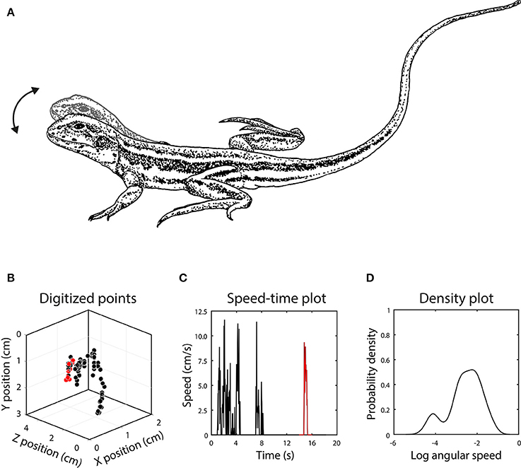
Figure 2. (A) Head bob displays of Ctenophorus fordi consist of up and down motion of the head, with each bout often containing several bobs. (B) After digitizing the position of the head in each video frame, the display was reconstructed in 3D, with each point representing the position of the head in one frame. In this example, the lizard first raised its body off the ground and then executed several head bobs. The red points represent an individual head bob. (C) Signal motion is depicted by the change in position of the target point in 3D space between successive frames, with a single head bob once again indicated in red. (D) The set of motion speeds in the display is summarized using a kernel density function after conversion to angular speed.

FIGURE 3

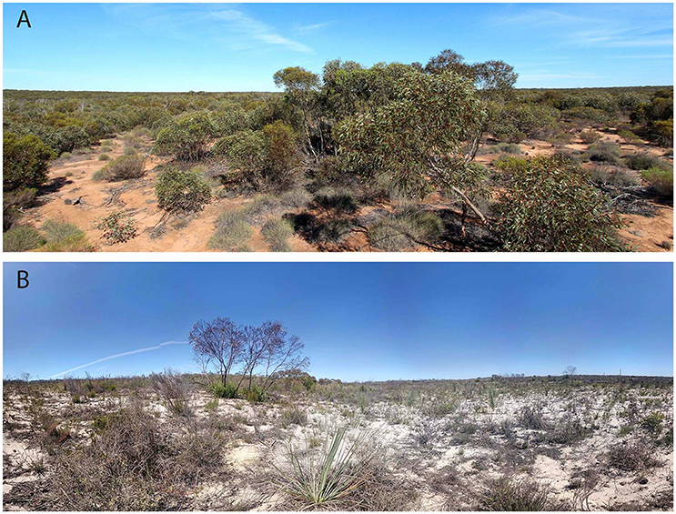
Figure 3. Contrasting habitats of Ctenophorus fordi. (A) Murray-Sunset National Park in northeast Victoria is characterized by dune-swale topography, with mallee trees and thick spinifex undergrowth. (B) Ngarkat Conservation Park in southwest South Australia is characterized by an open mallee canopy, with spinifex and heathy understory.

Data Collection

Recording Displays

All recordings involved filming interactions between male lizards in the field. We filmed four lizards, two each from MSNP and NCP. We recorded displays using two camcorders simultaneously, which were synchronized and calibrated after each recording, to reconstruct signals in 3D. To synchronize cameras, we used the offset of a beam from a laser pointer viewable from both cameras, and located subsequently in video editing software. Additional synchronization can be undertaken during the digitizing process in order to match the two cameras to within 40 ms (PAL frame-rate). The calibration process involved placing a calibration object containing 20 non-coplanar points distributed evenly through its volume so that most points were visible from both cameras. Importantly, still images of the calibration object are obtained after displays are filmed without modifying camera settings or its position in any way. See Peters et al. (2016) for further details about the filming protocol, and Figure S1 accompanying that paper for photos of our calibration object.

Habitat Information

Information on the structure of the habitat was collected for each display by mapping the position of the lizard relative to the main features of the area, creating schematic illustrations of the vegetation layout and capturing a panoramic image. This involved identifying the plants around the resident that could potentially mask the signal as well as the general topography of the landscape. Plant-signaler distances were recorded for all relevant plants, which were then filmed under controlled windy conditions. We used a leaf blower in order to standardize measurements across plants and habitats, and positioned it at distances of 2 and 3 m from the plants to reflect wind conditions of 4 and 2.5 m/s respectively. Filming at all sites involved positioning the camera at a distance of 2 m from the plant and perpendicular to the direction of wind emanating from the leaf blower. This arrangement was selected as it was anticipated to be optimal for capturing dominant fast speed plant movements. We used consistent camera settings (e.g., zoom) and only when natural wind speed was close to 0 m/s when filming plants at all sites.

Data Analysis

Digitizing Displays

We digitized head-bob displays using direct linear transformation (DLT) in Matlab (MathWorks Inc.) following Hedrik (2008). Application of this technique to quantifying lizard displays is reported in Peters et al. (2016). The first step is to locate each point from the calibration object in the still images obtained from both cameras. A set of calibration coefficients is generated when the x-y coordinate data from both cameras are combined with information from a specification file of known distances. When calibration is completed, we locate the chosen feature from the display in each frame of video from both cameras. During this part of the process, any disparity in the synchronicity of the cameras can be addressed by advancing one of the videos until they match at the frame level. The x-y coordinate data for this feature is then combined with the DLT calibration coefficients to reconstruct the movement in 3D (Figure 2). The x-y-z coordinate data can be used to measure any number of variables, including speed, amplitude, direction of movement and acceleration and is now independent of the position of the cameras during filming. Display speeds (S), representing the change in position in 3D space (Euclidean distance) of the target point between successive frames, were converted to angular speeds according to:

$\begin{array}{ll}\mathrm{\theta }= 2t{a}^{-1}\left(\frac{S}{2D}\right)& (1)\end{array}$

where D represents signaler-receiver distance (1 and 4 m). We calculated kernel density estimates of the log of angular speeds in the range [−15 15] for comparison with noise data using the ksdensity function in Matlab, 2015b (MathWorks Inc.), which generates a vector describing the relative probability of different angular speeds.

Scene Layout

Our objective was to quantify the contrast of a given signal in an environment without being limited to a single viewing position. Although the number of viewing positions is unconstrained, we determined during pilot work that four viewing positions around the signaler were sufficient and selected the four cardinal directions (North, South, East and West) to standardize across sites. As illustrated in Figure 1, the position of the receiver dictates which plants are relevant, so for each viewing position we identified the plants determined to be within a 150° viewing angle from each viewing position (lizard field of view based on work on Amphibolurus muricatus, as per New, 2014; additional viewing positions might be required if the focal species has narrower fields of view). Since each plant has been recorded under calm and windy conditions, the number of relevant plant motion videos for each viewing position was double the number of relevant plants.

Plant Motion

Movement speeds of plants were calculated using a gradient detector model, as described by Peters et al. (2002). Output from gradient detectors comprises velocity estimates for motion in image sequences, and the magnitude component is comparable to how we measure signal speeds in that both provide estimates for distance traveled over time. For the present purposes, we limited analysis to 5 s for each plant video (125 frames; PAL frame rate) and converted units from pixels to cm using an object of known size in the video. Our intention was to compare the distribution of motion speeds generated by lizard displays and plant movements. However, to ensure consistency in filming of plants at multiple sites we set the camera's zoom to be as wide as possible. Comparing lizard movement with the whole video frame would thus not reflect the motion segmentation task facing receivers, which is likely to involve local rather than wide field contrast. Consequently, we divide the HD plant video into sub-regions and compare lizard displays against plant movement contained within these subregions. As a result, speed data for a given plant were represented by 510 subregions each featuring 5 s of movement. Our subdivision procedure ensured that the physical area covered by each subregion was equivalent to the space utilized by a lizard during a display.

We converted speed from physical units (x) to angular speed (θ) according to:

$\begin{array}{ll}\mathrm{\theta }= 2ta{n}^{-1}\left(\frac{x}{2D}\right)& (2)\end{array}$

Here, D represents the distance of the plant from the viewing position, calculated as:

$D=\{\begin{array}{c}SRd+SPd, if \left(plant behind signaller\right)\\ SRd-SPd, if \left(plant in front of signaller\right)\\ SRd, if \left(plant in line with signaller\right)& (3)\end{array}$

where SRd and SPd represent signaler-receiver distance and signaler-plant distance respectively. SRd was selected from {1, 4 m} and SPd was obtained during data collection. Kernel density estimates of the log of angular speeds in the range [−15 15] was calculated for each subregion.

Signal vs. Noise: Quantifying Signal Contrast

We compared image motion distributions due to lizard displays with those of relevant wind-blown plants (Figure 4). For a given microhabitat there are four viewing positions, and from each position there are N plants that are relevant (Figure 4A). Image motion from video footage of these plants is spatially subdivided, as explained above, and each subregion was compared with the lizard's motion distribution (Figure 4B). In each comparison the kernel density function for the subregion of plant motion (Figure 4C) was subtracted from the kernel density estimate for the lizard display (Figure 4D). By integrating this difference function for values greater than zero (where lizard motion features a higher relative proportion of movement at the given angular speed) we estimate the relative probability that lizard movement differs from plant movement, which we now refer to as relative contrast (values range from 0 to 1, where higher values indicate more effective signals). This process yields a matrix of contrast values for each plant/viewing position combination (Figure 4E). We summarized the location and shape of this distribution by obtaining the median, as a measure of central tendency, and computing the scale parameter as a measure of deviation (Rousseeuw and Croux, 1993), resulting in a pair of values per plant at the given viewing position (Figure 4F). The scale parameter was selected as the distributions were highly skewed and measures such as standard deviation or standard error are inappropriate. This was repeated for all relevant plants for each of the four viewing positions. If there were no relevant plants for a given viewing position then contrast was assumed to be 1; if the topography of the land, or layout of the scene, meant that the lizard could not be seen from a given viewing position then the contrast score for that position was set at 0. The set of location and scale values for all plant/viewing position combinations summarized the predicted contrast of the given signal at the given microhabitat. A final contrast score for the microhabitat was calculated as the mean (±SD) location and scale values (Figure 4G). Thus, our metric for determining relative contrast captures the difference between motion signal and noise distributions as well as the heterogeneity of motion-noise environments.

FIGURE 4

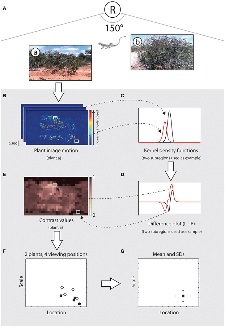
Figure 4. Summary of the procedure used during scene analysis to estimate the contrast of a signal in a given microhabitat. (A), Schematic illustration showing a hypothetical scene in which a receiver (R) is shown relative to the signaling lizard and two plants (a, b). (B) Plant motion is analyzed using a gradient detector model and the image frame is subdivided into smaller subregions for comparison with lizard movement. White rectangles indicate subregions with high (top) and low (bottom) image motion. (C) Distribution of motion speeds from these two subregions, as summarized using a kernel density function (black and red lines for high and low motion noise respectively). (D) Kernel density functions for the two subregions of plant motion were subtracted from the kernel density estimate for the lizard display (not shown). This difference is used to estimate the relative probability that lizard movement differs from plant movement, which we refer to as relative contrast. (E) For each plant/viewing position combination we obtain a matrix of contrast values, ranging from 0 to 1, where higher values indicate greater contrast between the signal and noise environment. (F) The location (central tendency) and scale (variation) of this distribution is calculated, resulting in a pair of values for each plant at each viewing position. In this example, eight data points are shown for two relevant plants for each of four viewing positions. (G) A single contrast score for a given scene is obtained by calculating the mean (±SD) location and scale values.

Scene Analysis

We first examined the distributions of movement speeds for lizard displays from MSNP and NCP. Scene analysis to determine the relative contrast of signals in noise following the procedure described above was undertaken in three ways. First we calculated contrast scores for lizards in their own microhabitat. Second, we “placed” lizards into the microhabitat of the other lizard from the same general habitat. Third, we placed lizards in each of the microhabitats from the alternative habitat. We have used a limited data set to illustrate our approach and consequently we present contrast scores graphically and discuss the implications of our results but do not undertake inferential statistics due to small sample sizes. Nonetheless, we suggest a potential next step in the analysis of contrast scores in the discussion.

Results

Lizard Displays

Kernel density estimates summarizing head bob displays from two populations of C. fordi are shown in Figure 5. For each individual lizard, 3–7 bouts of signaling behavior were analyzed, each consisting of multiple head bobs and lasting less than 2 s. From these data, it appears that lizards from MSNP generated displays with relatively greater speeds than those from NCP.

FIGURE 5

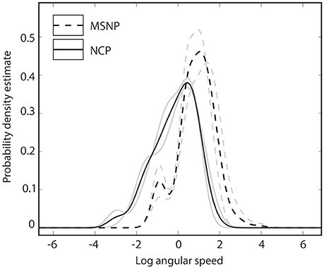
Figure 5. Probability density functions summarizing angular speeds of lizard displays for lizards from Murray-Sunset National Park (dashed lines) and Ngarkat Conservation Park (solid lines). Data for two individuals (gray lines) and population mean (black lines) are shown for each population.

Scene Analysis

Contrast scores for lizards in their own microhabitat, microhabitats from their general habitat (within population) as well as the alternate habitat (between populations) are shown in Figure 6 for each lizard separately. Despite having “slower” signals, lizards from NCP perform better than lizards from MSNP in their own habitat. This applied not only to the microhabitat where the signals were originally emitted, but also to a neighboring microhabitat. Little variation was observed in signal contrast within habitats (original vs. neighboring microhabitat) regardless of lizard origin. Conversely, contrast scores changed markedly for all lizards when placed in microhabitats of the alternate habitat. In addition, MSNP lizards performed better in NCP, and NCP lizards performed worse in MSNP, which hints at a stronger masking effect from MSNP habitat. Mean contrast scores do not seem to change drastically with distance. However, we observed a reduction in variance as the receiver moves farther away (from 1 to 4 m), as indicated by the smaller SDs at 4 m. This is likely due to the non-linear relationship between angular size and distance.

FIGURE 6

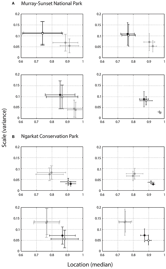
Figure 6. Relative contrast of lizard displays calculated using the mean (±SD) location and scale values of two individuals from Murray-Sunset National park (A) and two individuals from Ngarkat Conservation Park (B), at viewing distances of 1 m (left column) and 4 m (right column). Higher scores for location (X axis) indicate greater contrast between the signal and noise conditions within a given environment in favor of the signal. Scale values (Y axis) reflect the extent of variability in scenes, with higher values reflecting greater variability in noise within the habitat and suggests areas of high and low noise. As such, data points in the bottom right hand corner of these plots represent more effective signals. Each plot shows the relative contrast of a single lizard in its own microhabitat (white), at another microhabitat within its own habitat (black), and in two microhabitats from the alternate habitat (gray).

Discussion

Our intention with this paper is to encourage a fresh look at motion signaling and outline a strategy for quantifying motion signals and the signaling environment that provides an opportunity to consider the true context in which signaling takes place. Our approach is powerful because we no longer make the assumption that our camera is ideally placed at the time of signaling. Signals and noise are filmed independently, which when combined with detailed mapping of the environment, enabled us to recreate multiple signal-in-noise scenarios by changing the viewing position of the intended receiver. Furthermore, it is inherently more powerful than the use of multiple cameras filming simultaneously. First, the logistical challenge of filming free living animals from multiple pre-determined viewing positions cannot be underestimated. Second, by separating signal and noise measurements we are afforded the opportunity to consider how signals of lizards would “perform” in any of the microhabitats we document, and not just the one in which they were filmed.

The relative contrast of C. fordi signals varied between allopatric populations. NCP signals were more effective than MSNP signals when quantified in their own habitats, but both showed a clear change in contrast when placed in the alternate habitats: NCP signals showed a decrease in contrast while MSNP signals improved. These results are consistent with the hypothesis that the environment at MSNP exerts a greater influence on signal efficacy than at NCP, and possibly drives the differences in display structure between populations (Figure 5). MSNP habitat is essentially a mallee woodland with a spinifex understory. Spinifex clumps produce considerable motion under windy conditions, particularly while they are flowering. In contrast, the areas of NCP where the signals were recorded had been recently burnt (within 5 years), and the vegetation was sparse. However, we must consider our results with caution as we compare only two individuals from each population. Inferential statistics were not possible here but with additional lizards and retaining the bivariate nature of the data (location and scale values; Figure 6), Hotelling's T² statistics (Batschelet, 1981) would be an appropriate way to consider statistically whether variation in contrast scores represent significant changes. Furthermore, although we might show statistically significant changes in contrast, knowledge of motion processing mechanisms in the focal species would be needed to determine biological significance (see below), as the threshold for detection would need to be determined empirically. Notwithstanding, the combination of variation in signal structure and predicted signal contrast in noise provides compelling evidence for habitat-dependent variation in motion signaling.

Ctenophorus fordi has a relatively simple display, whereas other species utilize more complex displays involving multiple motor patterns. Our methodology allows for consideration of different motor patterns in isolation. This would be particularly informative in quantifying the reasons why species add novel components to their display under noisy environmental conditions (Anolis gundlachi; Ord and Stamps, 2008). The relative contrast of displays with and without the additional component could be calculated to compare contrast under each environmental context. Furthermore, Barquero et al. (2015) reported that different populations of Amphibolurus muricatus exhibited subtle variation in display structure and suggested habitat differences as a potential driving force. This is precisely the kind of habitat-dependent variation in signal structure often documented for other modalities (color: Leal and Fleishman, 2004; Ng et al., 2013; McLean et al., 2015; sounds: Ryan et al., 1990; Potvin and Parris, 2012), but has not been quantified in analogous detail for signals defined by motion. The methodology we propose here will facilitate the generation of such data.

Similarities in signal structure as a consequence of the signaling environment are also anticipated in sympatric species. Many habitats accommodate multiple signaling species, and while niche partitioning is reported (Case and Bolger, 1991; Leal and Fleishman, 2002), the dynamic component of behavior has not been thoroughly examined. Our methodology provides the opportunity to explore this in detail for motion signals. We anticipate that signal contrast scores for species occurring within the same habitat, subjected to the same environmental constraints, should be equivalent across all sites in the habitat (Ecomorph Convergence Hypothesis; Nicholson et al., 2007; Ord et al., 2013). Certainly, sympatric species need to avoid mistaking unrelated individuals (Species Recognition Hypothesis; Rand and Williams, 1970; Nicholson et al., 2007), but our prediction of equivalent contrast scores is still consistent with this idea as species recognition cues may be given by the choice of motor pattern rather than movement characteristics.

Limitations

We have outlined why motion signal analysis needs to consider the signaling context in more detail and our methodology provides a clear way forward; yet there are two unavoidable restrictions of our approach. First, although we compare motion speeds of both signal and noise, we have used different techniques to quantify each type of movement. Lizard signals are reconstructed in 3D, while plant motion is filmed in 2D from a single viewpoint perpendicular to the camera. Feature tracking and 3D reconstruction of plant movements is achievable (Bian et al., 2016), but impractical on a large scale. Plants are complex structures, so selecting parts of plants to be representative of the plants' movements is problematic. Until we know more about plant motion at the microhabitat level (Peters et al., 2008; Peters, 2013; Powell and Leal, 2014), we accept that plant motion noise might vary to some extent as you move around a plant and as such we have simplified the treatment of noise. Importantly, by adopting a standardized approach to recording plant motion in the field we ensure consistency within and between habitats. Furthermore, the use of a gradient detector model for image motion computation is appropriate here as it generates motion vectors that are very similar to outcomes from feature tracking (cf. correlation-type motion detector models).

A second important limitation of the results we present herein is that we must refer to signal contrast rather than signal efficacy. Ideally we would like to be able to predict the effectiveness of a given signal-in-noise scenario in terms of the perceptual capabilities of a receiver (Caves et al., 2016). Such an outcome would be analogous to visual modeling of color, whereby color signals are compared with other spectral components of the environment to yield differences in terms of perceptual equivalents (Vorobyev and Osorio, 1998; McLean et al., 2014; Delhey et al., 2015). However, we have not considered motion contrast in the context of receiver sensory systems. In part this is due to the complexity of image motion segmentation of natural scenes, but reflects also a lack of knowledge of the sensitivities of our focal species to motion. Indeed, knowledge of the relative response of animals to different movements, which has been done quite effectively using various species of Anolis lizards (Pallus et al., 2010; Steinberg and Leal, 2016) would extend our metric toward a measure of efficacy. For example, spatial frequencies outside of the perceptual capabilities of receivers could be removed from the plant image sequences before the gradient detector is applied to reflect better the information available for motion perception. Similarly, information on the temporal resolution of receivers could be used to weight different motion components to more closely match the perceptual capabilities of the focal species, before calculating signal-noise contrast. Field of view might also be different between species, and will influence the number of relevant plants for a given viewing positions. For species with narrower fields of view, additional viewing positions can be included (see Section Scene Layout) to accurately sample the habitat. Importantly, our method of data collection in the field and the raw data we collect would be suitable input to such analyses. Consequently, it is possible for us to revisit our signal contrast results in line with perceptual knowledge of this kind when it does become available.

Extending the Methodology

Notwithstanding the above caveats, there are several ways in which we can extend the utility of the approach, in terms of sampling frequency, the information we extract from our raw data, how data might be used and in adding complexity. We have considered motion speeds in this paper, however, we are inherently limited by the frame rate of our cameras. Any movement that occurs within the sampling frequency of our cameras (every 40 ms) will be under-sampled. The use of cameras with higher frame rates is recommended where possible, however, in our implementation this constraint applies both to signal and noise measurements. Motion speed is only one parameter characterizing signals and noise and a clearer understanding of motion segmentation mechanisms might point to alternative or additional parameters upon which to focus. Most notably would be variation in terms of amplitude and movement direction. Angular speed differences between signal and noise have been the subject of recent attention (Peters and Evans, 2003; Ord et al., 2007, 2010; Fleishman and Pallus, 2010; Pallus et al., 2010), while differences between signal and noise in terms of the direction of movement also might be a useful avenue of inquiry, although it has not received as much attention in the literature (but see Peters et al., 2008; How et al., 2009). Movement amplitude and direction information could be extracted from the raw data we have collected. Furthermore, existing datasets could be used in simulations that indicate the level of variation in signal structure necessary for higher contrast scores. For example, using measured speeds as the starting point, new datasets of slightly modified speeds could be generated and compared with existing plant motion data. In addition, if angular amplitudes were instead the parameter of interest, then simulations could be undertaken to achieve greater amplitudes while keeping speed the same. Regardless of the chosen parameter, the result would yield predictions on what must be accomplished to improve outcomes which could be considered in the context of physiological constraints and provide useful arguments for suggesting alternative strategies for enhanced efficacy (see Peters et al., 2008).

Our methodology could also be extended to consider complex habitats. The approach we have taken in this description of the method reflects the circumstances in which our study species operate, and is relatively simplistic in that we consider the positions of signaler and receiver to vary only in the horizontal plane (Figure 7A). Furthermore, we calculated signal speeds in terms of the actual distance moved in 3D space before converting these values to angular speeds based on a specified viewing distance. In this way our analyses always represented the signal at its maximum speed. However, there are many species in which there are substantial and important differences between signaler and receiver in the vertical plane (Figure 7B). Measuring signal performance in these circumstances is more than just relative contrast with plant motion noise, and would benefit from an analytical approach in which receiver positions are limited but more precisely defined. There are additional challenges to filming in such environments, but to consider signal performance in this scenario requires only one additional step in the data collection phase. Filming of lizard displays and identifying and filming relevant plants would follow the procedures we outline above. For a more focused analysis it would be necessary to note down the locations in which receivers are likely to be located in terms of horizontal and vertical distances from the signaler. During the analysis phase, it would be straightforward to generate view-specific angular speeds directly from raw data (Figure 7B).

FIGURE 7

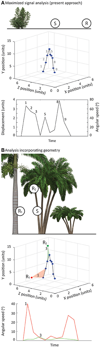
Figure 7. (A) Top panel—In the present study we have assumed that the position of receiver relative to signaler is on the same vertical plane and consider changes in position in terms of horizontal distance only. Middle panel—We determined 3D position of chosen features over time and measured physical movements in 3D space (Bottom panel). Using our nominated receiver position, in terms of horizontal distance, we converted these values to angular speeds. In this way, the angular speeds for the signal represent the maximum. (B) Top panel—Signaling interactions of many species feature substantial variation in the vertical plane and this can have a substantial impact on perceived signal speeds. Middle panel—The approach we outline in the present study can be modified to incorporate the geometry of the interaction. By noting receiver positions in 3D space relative to the signaler, angular speeds can be calculated directly for each viewing position. Bottom panel—This provides view specific estimates of angular speed, which can vary considerably for the same physical displacement.

Broader Applications

Our approach is not limited to intraspecific communication and could be applied to other functionally important vision-based behavior. For example, chameleons and several species of phasmid are suggested to use motion to mimic their surroundings and to prevent recognition by predators (Gans, 1967; Robinson, 1969; Bässler and Pflüger, 1979; Bian et al., 2016), while other species use movement to avoid being detected by their prey (Kennedy, 1965; Fleishman, 1985). For example, the Mexican vine snake (Oxybelis aeneus) often moves or changes position when the wind is blowing and plants are moving, which purportedly renders the snake's movement difficult for prey to classify as a potential threat (Fleishman, 1985). Similarly, cryptic prey exploit the sensory processes of their predators in order to avoid detection and blend with the background, while masquerading animals target their cognitive processes to ensure misidentification after detection (Skelhorn et al., 2010; Skelhorn, 2015). Our approach would allow for detailed analyses of the relative conspicuousness of the model and the mimic and to understand more clearly the behavior and environmental requirements of such species.

Conclusions

We have shown that accurately quantifying the relative contrast of motion-based signals is not only possible but necessary if our understanding of this form of animal communication is to progress. Our methodology allows us to record displays and quantify signals without the constraints of filming position, as well as to calculate the masking potential of the environment and relative contrast of the signals. We illustrated its utility for comparing motion displays of a given species in multiple habitats, and outline how the approach could be extended in a number of ways; we also recommend this approach for any system in which motion conspicuousness is a central determinant of behavior. As the structure of habitats around the world continues to change as a consequence of climate change and anthropogenic activities, it is essential we understand how species that utilize these habitats are being affected. This includes quantifying the effects of environmental noise.

Ethics Statement

This study was carried out in accordance with the recommendations of La Trobe University Ethics Committee and South Australia Ethics Committee. The protocol was approved by the Department of Environment and Primary Industries (Victoria, Australia) and the Department of Environment, Water and Natural Resources (South Australia, Australia).

Author Contributions

JR and RP designed the experiment. JR conducted the experiment and collected the data. JR and RP analyzed the data. JR and RP wrote the manuscript. All authors reviewed and approved the manuscript.

Conflict of Interest Statement

The authors declare that the research was conducted in the absence of any commercial or financial relationships that could be construed as a potential conflict of interest.

Acknowledgments

We thank Xue Bian for providing images for Figure 1, and Paul Davies, Matt Sleeth, and Kate Beskeen for their assistance during fieldwork. Data collection was performed in accordance with the ethical regulations of La Trobe University (AEC 12-37) and South Australia (55/2012), under permits provided by DEPI in Victoria (10006812) and DEWNR in South Australia (Q26078).

References

Amézquita, A., and Hödl, W. (2004). How, when, and where to perform visual displays: the case of the amazonian Frog Hyla parviceps. Herpetologica 60, 420–429. doi: 10.1655/02-51

CrossRef Full Text | Google Scholar

Barquero, M. D., Peters, R. A., and Whiting, M. J. (2015). Geographic variation in aggressive signalling behaviour of the Jacky dragon. Behav. Ecol. Sociobiol. 69, 1501–1510. doi: 10.1007/s00265-015-1962-5

CrossRef Full Text | Google Scholar

Bässler, U., and Pflüger, H. J. (1979). The control-system of the femur-tibia-joint of the phasmid Extatosoma tiaratum and the control of rocking. J. Comp. Physiol. 132, 209–215. doi: 10.1007/BF00614492

CrossRef Full Text | Google Scholar

Batschelet, E. (1981). Circular Statistics in Biology. New York, NY: Academic Press.

Google Scholar

Bian, X., Elgar, M. A., and Peters, R. A. (2016). The swaying behavior of Extatosoma tiaratum: motion camouflage in a stick insect? Behav. Ecol. 27, 83–92. doi: 10.1093/beheco/arv125

CrossRef Full Text | Google Scholar

Brumm, H. (2004). The impact of environmental noise on song amplitude in a territorial bird. J. Anim. Ecol. 73, 434–440. doi: 10.1111/j.0021-8790.2004.00814.x

CrossRef Full Text | Google Scholar

Brumm, H., and Slabbekoorn, H. (2005). “Acoustic communication in noise,” in Advances in the Study of Behavior, eds P. Slater, C. Snowdon, T. Roper, H. Brockmann, and M. Naguib (San Diego, CA: Academic Press), 151–209.

Google Scholar

Brumm, H., Voss, K., Köllmer, I., and Todt, D. (2004). Acoustic communication in noise: regulation of call characteristics in a New World monkey. J. Exp. Biol. 207, 443–448. doi: 10.1242/jeb.00768

PubMed Abstract | CrossRef Full Text | Google Scholar

Carpenter, C. C., Badham, J. A., and Kimble, B. (1970). Behavior patterns of three species of Amphibolurus (Agamidae). Copeia 1970, 497–505. doi: 10.2307/1442277

CrossRef Full Text | Google Scholar

Case, T. J., and Bolger, D. T. (1991). The role of interspecific competition in the biogeography of island lizards. Trends Ecol. Evol. 6, 135–139. doi: 10.1016/0169-5347(91)90093-d

PubMed Abstract | CrossRef Full Text | Google Scholar

Caves, E. M., Frank, T. M., and Johnsen, S. (2016). Spectral sensitivity, spatial resolution and temporal resolution and their implications for conspecific signalling in cleaner shrimp. J. Exp. Biol. 219, 597–608. doi: 10.1242/jeb.122275

PubMed Abstract | CrossRef Full Text | Google Scholar

Cocroft, R. B., and Rodriguez, R. L. (2005). The behavioral ecology of insect vibrational communication. Bioscience 55, 323–334. doi: 10.1641/0006-3568(2005)055[0323:TBEOIV]2.0.CO;2

CrossRef Full Text | Google Scholar

Cogger, H. G. (1978). Reproductive cycles, fat body cycles and socio-sexual behaviour in the Mallee Dragon, Amphibolurus fordi (Lacertilia: Agamidae. Aust. J. Zool. 26, 653–672. doi: 10.1071/ZO9780653

CrossRef Full Text | Google Scholar

Delhey, K., Delhey, V., Kempenaers, B., and Peters, A. (2015). A practical framework to analyze variation in animal colors using visual models. Behav. Ecol. 26, 367–375. doi: 10.1093/beheco/aru198

CrossRef Full Text | Google Scholar

Endler, J. A. (1990). On the measurement and classification of colour in studies of animal colour patterns. Biol. J. Linnean Soc. 41, 315–352. doi: 10.1111/j.1095-8312.1990.tb00839.x

CrossRef Full Text | Google Scholar

Endler, J. A. (1992). Signals, signal conditions, and the direction of evolution. Am. Nat. 139, S125–S153. doi: 10.1086/285308

CrossRef Full Text | Google Scholar

Endler, J. A., and Thery, M. (1996). Interacting effects of lek placement, display behavior, ambient light, and color patterns in three neotropical forest-dwelling birds. Am. Nat. 148, 421–452. doi: 10.1086/285934

CrossRef Full Text | Google Scholar

Fleishman, L. J. (1985). Cryptic movement in the vine snake Oxybelis aeneus. Copeia 1985, 242–245. doi: 10.2307/1444822

CrossRef Full Text | Google Scholar

Fleishman, L. J. (1986). Motion detection in the presence and absence of background motion in an Anolis lizard. J. Comp. Physiol. A 159, 711–720. doi: 10.1007/BF00612043

PubMed Abstract | CrossRef Full Text | Google Scholar

Fleishman, L. J. (1988a). Sensory and environmental influences on display form in Anolis auratus, a grass anole from panama. Behav. Ecol. Sociobiol. 22, 309–316.

Google Scholar

Fleishman, L. J. (1988b). Sensory influences on physical design of a visual display. Anim. Behav. 36, 1420–1424. doi: 10.1016/S0003-3472(88)80212-4

CrossRef Full Text | Google Scholar

Fleishman, L. J (1992). The influence of the sensory system and the environment on motion patterns in the visual displays of anoline lizards and other vertebrates. Am. Nat. 139, S36–S61. doi: 10.1086/285304

CrossRef Full Text | Google Scholar

Fleishman, L. J., and Pallus, A. C. (2010). Motion perception and visual design in Anolis lizards. Proc. R. Soc. B 277, 3547–3554. doi: 10.1098/rspb.2010.0742

PubMed Abstract | CrossRef Full Text | Google Scholar

Gans, C (1967). The chameleon. J. Nat. Hist. 76, 53–59.

Gibbons, J. R. H. (1979). The hind leg pushup display of the Amphibolurus decresii species complex (Lacertilia: Agamidae). Copeia 1979, 29–40. doi: 10.2307/1443725

CrossRef Full Text | Google Scholar

Grafe, T. U., and Wanger, T. C. (2007). multimodal signaling in male and female foot-flagging frogs staurois guttatus (Ranidae): an alerting function of calling. Ethology 113, 772–781. doi: 10.1111/j.1439-0310.2007.01378.x

CrossRef Full Text | Google Scholar

Greenfield, M. D. (1988). Interspecific acoustic interactions among katydids (Neoconocephalus): inhibition-induced shifts in diel periodicity. Anim. Behav. 36, 684–695. doi: 10.1016/S0003-3472(88)80151-9

CrossRef Full Text | Google Scholar

Hailman, J. P., and Dzelzkalns, J. J. I. (1974). Mallard tailwagging: punctuation for animal communication? Am. Nat. 108, 236–238. doi: 10.1086/282904

CrossRef Full Text | Google Scholar

Hedrik, T. L. (2008). Software techniques for two- and three-dimensional kinematic measurements of biological and biomimetic systems. Bioinsp. Biomimet. 3, 1–6. doi: 10.1088/1748-3182/3/3/034001

CrossRef Full Text

How, M. J., Hemmi, J. M., Zeil, J., and Peters, R. (2008). Claw waving display changes with receiver distance in fiddler crabs, Uca perplexa. Anim. Behav. 75, 1015–1022. doi: 10.1016/j.anbehav.2007.09.004

CrossRef Full Text | Google Scholar

How, M. J., Zeil, J., and Hemmi, J. M. (2007). Differences in context and function of two distinct waving displays in the fiddler crab, Uca perplexa (Decapoda: Ocypodidae). Behav. Ecol. Sociobiol. 62, 137–148. doi: 10.1007/s00265-007-0448-5

CrossRef Full Text | Google Scholar

How, M. J., Zeil, J., and Hemmi, J. M. (2009). Variability of a dynamic visual signal: the fiddler crab claw-waving display. J. Comp. Physiol. A 195, 55–67. doi: 10.1007/s00359-008-0382-7

PubMed Abstract | CrossRef Full Text | Google Scholar

Jackson, R. (1986). The display behavior of Bavia aericeps (Araneae, Salticidae), a jumping spider from Queensland. Aust. J. Zool. 34, 381–409. doi: 10.1071/ZO9860381

CrossRef Full Text | Google Scholar

Jackson, R. R. (1977). Courtship versatility in the jumping spider, Phidippus johnsoni (Araneae: Salticidae). Anim. Behav. 25(Pt 4), 953–957. doi: 10.1016/0003-3472(77)90046-X

CrossRef Full Text | Google Scholar

Jenssen, T. A. (1977). Evolution of anoline lizard display behavior. Am. Zool. 17, 203–215. doi: 10.1093/icb/17.1.203

CrossRef Full Text | Google Scholar

Kellogg, P. P., and Stein, R. C. (1953). Audio-spectographic analysis of the songs of the alder flycatcher. Wilson Bull. 65, 75–80.

Google Scholar

Kennedy, J. P. (1965). Notes on the habitat and behavior of a snake, Oxybelis aeneus wagler, in Veracruz. Southwest. Nat. 10, 136–139. doi: 10.2307/3669163

CrossRef Full Text | Google Scholar

Leal, M., and Fleishman, L. J. (2002). Evidence for habitat partitioning based on adaptation to environmental light in a pair of sympatric lizard species. Proc. R. Soc. B 269, 351–359. doi: 10.1098/rspb.2001.1904

PubMed Abstract | CrossRef Full Text | Google Scholar

Leal, M., and Fleishman, L. J. (2004). Differences in visual signal design and detectability between allopatric populations of Anolis lizards. Am. Nat. 163, 26–39. doi: 10.1086/379794

PubMed Abstract | CrossRef Full Text | Google Scholar

Lengagne, T., and Slater, P. J. B. (2002). The effects of rain on acoustic communication: tawny owls have good reason for calling less in wet weather. Proc. R. Soc. Lond. B 269, 2121–2125. doi: 10.1098/rspb.2002.2115

PubMed Abstract | CrossRef Full Text | Google Scholar

Lohr, B., Wright, T. F., and Dooling, R. J. (2003). Detection and discrimination of natural calls in masking noise by birds: estimating the active space of a signal. Anim. Behav. 65, 763–777. doi: 10.1006/anbe.2003.2093

CrossRef Full Text | Google Scholar

Lorenz, K. (1971). “Comparative studies of the motor patterns of Anatinae,” in Studies of Animal and Human Behavior, ed R. Martin (Cambridge, MA: Harvard University Press), 14–114.

Lythgoe, J. N. (1979). The Ecology of Vision. Oxford: Clarendon Press.

PubMed Abstract | Google Scholar

McGregor, P. K., Dabelsteen, T., Clark, C. W., Bower, J. L., and Holland, J. (1997). Accuracy of a passive acoustic location system: empirical studies in terrestrial habitats. Ethol. Ecol. Evol. 9, 269–286. doi: 10.1080/08927014.1997.9522887

CrossRef Full Text | Google Scholar

McLean, C. A., Moussalli, A., and Stuart-Fox, D. (2014). Local adaptation and divergence in colour signal conspicuousness between monomorphic and polymorphic lineages in a lizard. J. Evol. Biol. 27, 2654–2664. doi: 10.1111/jeb.12521

PubMed Abstract | CrossRef Full Text | Google Scholar

McLean, C. A., Stuart-Fox, D., and Moussalli, A. (2015). Environment, but not genetic divergence, influences geographic variation in colour morph frequencies in a lizard. BMC Evol. Biol. 15:156. doi: 10.1186/s12862-015-0442-x

PubMed Abstract | CrossRef Full Text | Google Scholar

Mennill, D. J., Burt, J. M., Fristrup, K. M., and Vehrencamp, S. L. (2006). Accuracy of an accoustic location system for monitoring the position of duetting songbirds in tropical forest. J. Acoust. Soc. Am. 119, 2832–2839. doi: 10.1121/1.2184988

PubMed Abstract | CrossRef Full Text | Google Scholar

New, S. T. D. (2014). Eye of the Dragon. Visual Specializations of the Jacky Dragon, Amphibolurus muricatus. Doctoral thesis. Canberra: The Australian National University.

Ng, J., Landeen, E. L., Logsdon, R. M., and Glor, R. E. (2013). Correlation between Anolis lizard dewlap phenotype and environmental variation indicates adaptive divergence of a signal important to sexual selection and species recognition. Evolution 67, 573–582. doi: 10.1111/j.1558-5646.2012.01795.x

PubMed Abstract | CrossRef Full Text | Google Scholar

Nicholson, K. E., Harmon, L. J., and Losos, J. B. (2007). Evolution of anolis lizard dewlap diversity. PLoS ONE 2:e274. doi: 10.1371/journal.pone.0000274

PubMed Abstract | CrossRef Full Text | Google Scholar

Ord, T. J., Charles, G. K., Palmer, M., and Stamps, J. A. (2016). Plasticity in social communication and its implications for the colonization of novel habitats. Behav. Ecol. 27, 341–351. doi: 10.1093/beheco/arv165

CrossRef Full Text | Google Scholar

Ord, T. J., Peters, R. A., Clucas, B., and Stamps, J. A. (2007). Lizards speed up visual displays in noisy motion habitats. Proc. R. Soc. B 274, 1057–1062. doi: 10.1098/rspb.2006.0263

PubMed Abstract | CrossRef Full Text | Google Scholar

Ord, T. J., and Stamps, J. A. (2008). Alert signals enhance animal communication in “noisy” environments. Proc. Natl. Acad. Sci. U.S.A. 105, 18830–18835. doi: 10.1073/pnas.0807657105

PubMed Abstract | CrossRef Full Text | Google Scholar

Ord, T. J., Stamps, J. A., and Losos, J. B. (2010). Adaptation and plasticity of animal communication in fluctuating environments. Evolution 64, 3134–3148. doi: 10.1111/j.1558-5646.2010.01056.x

PubMed Abstract | CrossRef Full Text | Google Scholar

Ord, T. J., Stamps, J. A., and Losos, J. B. (2013). Convergent evolution in the territorial communication of a classic adaptive radiation: Caribbean Anolis lizards. Anim. Behav. 85, 1415–1426. doi: 10.1016/j.anbehav.2013.03.037

CrossRef Full Text | Google Scholar

Pallus, A. C., Fleishman, L. J., and Castonguay, P. M. (2010). Modeling and measuring the visual detection of ecologically relevant motion by an Anolis lizard. J. Comp. Physiol. A 196, 1–13. doi: 10.1007/s00359-009-0487-7

PubMed Abstract | CrossRef Full Text | Google Scholar

Patricelli, G. L., and Krakauer, A. H. (2010). Tactical allocation of effort among multiple signals in sage grouse: an experiment with a robotic female. Behav. Ecol. 21, 97–106. doi: 10.1093/beheco/arp155

CrossRef Full Text | Google Scholar

Peters, R. A. (2008). Environmental motion delays the detection of movement-based signals. Biol. Lett. 4, 2–5. doi: 10.1098/rsbl.2007.0422

PubMed Abstract | CrossRef Full Text | Google Scholar

Peters, R. A. (2010). “Movement-based signalling and the physical world: modelling the changing perceptual task for receivers,” in Modelling Perception with Artificial Neural Networks, eds C. Tosh and G. Ruxton (Cambridge: Cambridge University Press), 269–292.

Google Scholar

Peters, R. A. (2013). “Noise in optic communication: motion from wind-blown plants,” Animal Communication in Noise, ed H. Brumm (Heidelberg: Springer), 311–330.

Google Scholar

Peters, R. A., Clifford, C. W. G., and Evans, C. S. (2002). Measuring the structure of dynamic visual signals. Anim. Behav. 64, 131–146. doi: 10.1006/anbe.2002.3015

CrossRef Full Text

Peters, R. A., and Evans, C. S. (2003). Design of the Jacky dragon visual display: signal and noise characteristics in a complex moving environment. J. Comp. Physiol. A 189, 447–459. doi: 10.1007/s00359-003-0423-1

PubMed Abstract | CrossRef Full Text | Google Scholar

Peters, R. A., Hemmi, J. M., and Zeil, J. (2007). Signaling against the wind: modifying motion-signal structure in response to increase noise. Curr. Biol. 17, 1231–1234. doi: 10.1016/j.cub.2007.06.035

PubMed Abstract | CrossRef Full Text | Google Scholar

Peters, R. A., Hemmi, J., and Zeil, J. (2008). Image motion environments: background noise for movement-based animal signals. J. Comp. Physiol. A 194, 441–456. doi: 10.1007/s00359-008-0317-3

PubMed Abstract | CrossRef Full Text | Google Scholar

Peters, R. A., Ramos, J. A., Hernandez, J., Wu, Y., and Qi, Y. (2016). Social context affects tail displays by Phrynocephalus vlangalii lizards from China. Sci. Rep. 6:31573. doi: 10.1038/srep31573

PubMed Abstract | CrossRef Full Text | Google Scholar

Potvin, D. A., and Parris, K. M. (2012). Song convergence in multiple urban populations of silvereyes (Zosterops lateralis). Ecol. Evol. 2, 1977–1984. doi: 10.1002/ece3.320

PubMed Abstract | CrossRef Full Text | Google Scholar

Powell, B. J., and Leal, M. (2014). Brain organization and habitat complexity in Anolis lizards. Brain Behav. Evol. 84, 8–18. doi: 10.1159/000362197

PubMed Abstract | CrossRef Full Text | Google Scholar

Purdue, J. R., and Carpenter, C. C. (1972). A comparative study of the display motion in the iguanid Genera Sceloporus, Uta, and Urosaurus. Herpetologica 28, 137–141.

Google Scholar

Ramos, J. A., and Peters, R. A. (2016). Dragon Wars: movement-based signalling by Australian agamid lizards in relation to species ecology. Aust. Ecol. 41, 302–315. doi: 10.1111/aec.12312

CrossRef Full Text | Google Scholar

Rand, A. S., and Williams, E. E. (1970). An estimation of redundancy and information content of anole dewlaps. Am. Nat. 104, 99–103. doi: 10.1086/282643

CrossRef Full Text | Google Scholar

Robinson, M. H. (1969). The defensive behaviour of some orthopteroid insects from Panama. Trans. R. Entomol. Soc. Lond. 121, 281–303. doi: 10.1111/j.1365-2311.1969.tb00521.x

CrossRef Full Text | Google Scholar

Rousseeuw, P. J., and Croux, C. (1993). Alternatives to the median absolute deviation. J. Am. Stat. Assoc. 88, 1273–1283. doi: 10.1080/01621459.1993.10476408

CrossRef Full Text | Google Scholar

Ruibal, R. (1967). “Evolution and behavior in West Indian anoles,” in Lizard Ecology: A Symposium ed W. W. Milstead (Missouri, MO: University of Missouri Press), 116–140.

Ruibal, R., and Philibosian, R. (1974). Aggression in the Lizard Anolis acutus. Copeia 1974, 349–357. doi: 10.2307/1442529

CrossRef Full Text | Google Scholar

Ryan, M. J., Cocroft, R. B., and Wilczynski, W. (1990). The role of environmental selection in intraspecific divergence of mate recognition signal in cricket frog, Acris crepitans. Evolution 44, 1869–1872. doi: 10.2307/2409514

CrossRef Full Text | Google Scholar

Skelhorn, J. (2015). Masquarade. Curr. Biol. 25, 643–644. doi: 10.1016/j.cub.2015.02.069

PubMed Abstract | CrossRef Full Text | Google Scholar

Skelhorn, J., Rowland, H. M., and Ruxton, G. D. (2010). The evolution and ecology of masquerade. Biol. J. Linnean Soc. 99, 1–8. doi: 10.1111/j.1095-8312.2009.01347.x

CrossRef Full Text | Google Scholar

Slabbekoorn, H., and Boer-Visser, A. D. (2006). Cities change the songs of birds. Curr. Biol. 16, 2326–2331. doi: 10.1016/j.cub.2006.10.008

PubMed Abstract | CrossRef Full Text | Google Scholar

Slabbekoorn, H., and Peet, M. (2003). Ecology: birds sing at a higher pitch in urban noise. Nature 424, 267–267. doi: 10.1038/424267a

PubMed Abstract | CrossRef Full Text | Google Scholar

Steinberg, D. S., and Leal, M. (2013). Sensory system properties predict signal modulation in a tropical lizard. Anim. Behav. 85, 623–629. doi: 10.1016/j.anbehav.2012.12.025

CrossRef Full Text | Google Scholar

Steinberg, D. S., and Leal, M. (2016). Visual motion detection and habitat preference in Anolis lizards. J. Comp. Physiol. A 202, 783–790. doi: 10.1007/s00359-016-1120-1

PubMed Abstract | CrossRef Full Text | Google Scholar

Vorobyev, M., and Osorio, D. (1998). Receptor noise as a determinant of colour thresholds. Proc. R. Soc. B 265, 351–358. doi: 10.1098/rspb.1998.0302

PubMed Abstract | CrossRef Full Text | Google Scholar

Wilson, S., and Swan, G. (2013). A Complete Guide to Reptiles of Australia. Sydney: New Holland Publishers.

Google Scholar

Witte, K., Farris, H. E., Ryan, M. J., and Wilczynski, W. (2005). How cricket frog females deal with a noisy world: habitat-related differences in auditory tuning. Behav. Ecol. 16, 571–579. doi: 10.1093/beheco/ari032

CrossRef Full Text | Google Scholar

Zanker, J. M., and Zeil, J. (2005). Movement-induced motion signal distributions in outdoor scenes. Netw. Comput. Neural Syst. 16, 357–376. doi: 10.1080/09548980500497758

PubMed Abstract | CrossRef Full Text | Google Scholar

Zeil, J., and Hemmi, J. M. (2006). The visual ecology of fiddler crabs. J. Comp. Physiol. A 192, 1–25. doi: 10.1007/s00359-005-0048-7

PubMed Abstract | CrossRef Full Text | Google Scholar

Zeil, J., and Zanker, J. M. (1997). A glimpse into crabworld. Vision Res. 37, 3417–3426. doi: 10.1016/S0042-6989(97)00106-5

PubMed Abstract | CrossRef Full Text | Google Scholar