Agro-Ecological Class Stability Decreases in Response to Climate Change Projections for the Pacific Northwest, USA

Introduction

Changing climatic conditions have resulted in substantial shifts in the geographic range of plant and animal species in natural ecosystems (Gonzalez, 2001; Wilson et al., 2005; Pauli et al., 2007; Chen et al., 2011) and are predicted to continue in the future (Schrag et al., 2008; Lawler et al., 2009; Monadjem et al., 2013). Likewise, single or multiple crop agro-ecosystems within a biophysical and socio-economic context have been affected by changing climatic variables (Kumar et al., 2013; Zhang et al., 2013). It follows that shifts in the geographic suitability of crop species/systems would occur in response to a changing climate (Evangelista et al., 2013; Ovalle-Rivera et al., 2015).

Assessing potential impacts of climate change on agro-ecosystems would benefit from classification systems that are dynamic and reflective of differences in the spatial distribution of land use/cover over time. Considering this goal, a new agro-ecosystem classification system, identified as dynamic agro-ecological classes (AECs) was developed for the dryland cropping region of the inland Pacific Northwest (iPNW; Huggins et al., 2014b). The AECs deviate from existing frameworks that classify agro-ecosystems based strictly on environmental drivers (e.g., soil, climate, and physiography) with relatively static boundaries, such as agro-climatic zones (Douglas et al., 1992), Ecoregions (US-EPA, Omernik and Griffith, 2014), and Major Land Resource Areas (USDA-NRCS, 2006). The AECs are based on the actual annual land use/cover derived from the Cropland data layer (USDA-NASS, 2008–2015). This classification approach for defining AECs provides the opportunity to quantify and test hypotheses regarding the drivers of spatio-temporal changes in cropping systems.

Currently, dryland cropping systems of the iPNW are fundamentally influenced by climatic gradients of temperature and precipitation (Schillinger et al., 2006). The dominant rotation practiced in regions with the lowest annual precipitation and highest annual temperatures is winter wheat–summer fallow which corresponds to the grain fallow class of AECs (Huggins et al., 2014b). This 2-year rotation includes a year of fallow to increase stored soil water that further ensures successful production of winter wheat. Grain-fallow systems become less prevalent in wetter portions of the iPNW where annual cropping systems dominate. Consequently, cropping system intensification progresses from the grain-fallow AEC with >40% annual fallow to the annual crop-fallow transition AEC (>10 to ≤ 40% annual fallow) and the annual cropping AEC (≤ 10% annual fallow). As climatic gradients influence crop choices and the use of fallow across the iPNW, we hypothesize that bioclimatic variables may explain significant geographic variations in AECs. In turn, a geospatial model of AECs based on bioclimatic variables may be used to project potential shifts in regional AECs under future climate scenarios.

Ecological studies that have assessed species distribution and projected changes in response to future climates often use and compare a variety of methods. These methods include generalized additive models (Estes et al., 2013), generalized linear models (Pompe et al., 2008), Artificial Neural Networks (Rasztovits et al., 2012), Random Forest (Schrag et al., 2008; Lawler et al., 2009; Chang et al., 2014; Langdon and Lawler, 2015), and maximum entropy modeling (MaxEnt; Monadjem et al., 2013; Clark et al., 2014; Ren et al., 2016). Here we use Random Forest modeling to assess potential regional shifts in AECs for the iPNW.

Our objectives are the following: (1) identify bioclimatic predictors which can discriminate among current AECs using two different Random Forest variable selection methods; (2) assess the predictive capacity of the geospatial models for current AECs using bioclimatic variables; (3) use future climate scenarios to predict changes in identified bioclimatic variables; (4) model regional shifts in AECs that would result if future climate scenarios were imposed on current agricultural systems; and (5) interpret the relevance of any AEC shifts in terms of sustainable agricultural intensification, vulnerability to resource degradation, and priorities for agricultural research.

Materials and Methods

Current Climate, Bioclimatic Variables, and AECs

The iPNW study region covering the lower elevations across eastern and central Washington, north-central Oregon, and northern Idaho has an extent of 9.4 million ha and is comprised of three dryland agroecosystem classes (AECs): (1) annual crop (AC); (2) annual crop-fallow-transition (AC-T); and (3) grain fallow (GF; Huggins et al., 2014b). The climate is generally Mediterranean-like (Schillinger et al., 2006), with cold, wet winters and warm to hot, dry summers. Annual average precipitation varies across the region with around 150 mm in lee of the Cascade Range in central Washington to more than 1,400 mm across the eastern portion of the study region in northern Idaho. Bioclimatic variables are derivatives of temperature and precipitation and variables considered biologically important for Mediterranean climates have been identified (Peinado et al., 2012). Here, we use 44 previously identified bioclimatic variables for empirical modeling (Table 1). Not included are potential future effects of elevated atmospheric CO₂ levels on bioclimatic variables.

TABLE 1

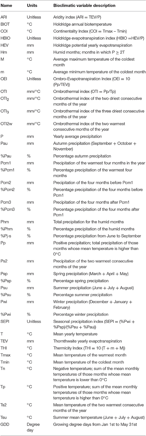
Table 1. Bioclimatic variables derived from climate data.

Cropland data layer derived AECs for dryland annual crop, annual crop-grain fallow-transition and grain fallow in raster layers (30 × 30 m resolution) were used for each of the years 2007–2014 (Huggins et al., 2015). The rasterized AEC information from 8 years were further combined into one map layer by categorizing each dryland AEC into two subclasses using the raster calculator tool in ArcGIS (version 10.3.1, ESRI, 2011): (1) stable dryland AECs, where pixels were consistently the same dryland class for 2007–2014 and; (2) dynamic dryland AECs, where pixels changed classes during the 8-year period (Huggins et al., 2015). Identifying stable and dynamic AEC subclasses resulted in the development of a classification comprised of six AECs. The resultant AEC layer was then brought to a coarser scale of 4 × 4 km, using the zonal statistics and cell statistics tool in ArcGIS (Figure 1).

FIGURE 1

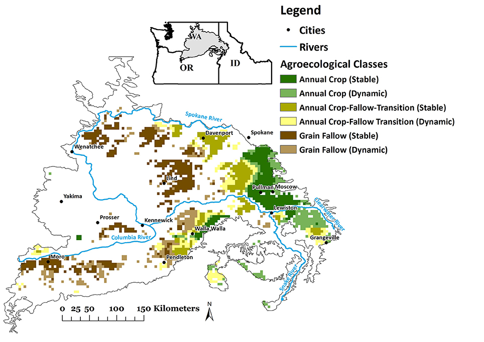
Figure 1. Agro-ecological classes (AECs) for years 2007 through 2014 at 4-km resolution.

Gridded climate data from years 1981–2010 was obtained from Abatzoglou (2013). Daily maximum temperature, minimum temperature, and accumulated precipitation at a 4 × 4 km resolution were aggregated to monthly time scales. We also extracted downscaled climate projections from 17 global climate models participating in the Fifth Coupled Model Inter-comparison Project (CMIP5) that have been evaluated for credibly simulating characteristics of regional climate (Rupp et al., 2013). Climate projections were downscaled using the Multivariate Adaptive Constructed Analogs approach (Abatzoglou and Brown, 2012) using the baseline training dataset of Abatzoglou (2013) to provide compatibility between current and future climate data. The 17 GCMs considered in evaluating predictive model performance were: bcc-csm1-1, BNU-ESM, CanESM2, CCSM4, CNRM-CM5, CSIRO-Mk3-6-0, GFDL-ESM2G, GFDL-ESM2M, inmcm4, IPSL-CM5A-LR, IPSL-CM5A-MR, IPSL-CM5B-LR, MIROC5, MIROC-ESM, MIROC-ESM-CHEM, MRI-CGCM3, and NorESM1-M. Climate network common data form (netcdf) layers (4 × 4 km resolution) were brought into ArcGIS and converted to raster layer using “Make netcdf to raster” tool and then to point dataset using “raster to point” tool. Conversion to point layer facilitated generation of latitude and longitude for each point, at the center of 4 × 4 km pixel, thus aiding the extraction of AEC information for each point in ArcGIS and extraction of present and future climate netcdfs of precipitation, maximum, and minimum temperature data in R (R Core Team, 2015).

A total of 44 bioclimatic variables (Table 1) were calculated using actual historical climate data (1981–2010) for precipitation, maximum, and minimum temperature. In addition, annual historical climate data derived from 17 Global climate models (GCM) for years 1981–2005 (Abatzoglou and Brown, 2012; Taylor et al., 2012) were used to calculate the same bioclimatic variables (Table 1). Reducing the data dimensionality from 44 to a few key variables was accomplished using two different wrapper variable selection algorithms: VarSelRF (Variable Selection using Random Forests; Diaz-Uriarte, 2014) and Boruta (Kursa and Rudnicki, 2010). VarSelRF, a minimal optimal approach, performs selection by retaining a compact subset of variables with improved classification performance based on “Out of Bag” (OOB) error and also allows computation of variable importance (VarSelRF R package, R Core Team, 2015). Boruta, an all relevant variable selection approach, identifies all relevant variables, and models them collectively to examine any underlying mechanisms in addition to being a predictive model (Boruta R package, R Core Team, 2015).

Observed bioclimatic variables and AECs (Figure 1) were used as input to R for variable selection using Boruta and VarSelRF algorithms and the process was repeated 30 times on split: training (70%) and test (30%) data sets, with different seed sets for each run. This step is based on the procedure used in the evaluation process of feature/gene selection (Fortino et al., 2014; Guo et al., 2014). The goal was to identify the variables that contributed the most to model performance in the selection process, which were selected repeatedly during 30 iterations. The motive behind partitioning the data as training (70%) and test (30%) was to understand the effect of selecting random subsets of data (training) on the ranking of variables and, as important variables were identified, the test set also provided an opportunity to independently quantify model performance.

Selection algorithms were used with their default parameters. The Boruta and VarSelRF algorithms facilitated selection of different sets of variables using performance metrics of z-score (which only identifies a variable as “important” or “unimportant”) and accuracy (estimated using OOB error), respectively. The variables selected by the two methods were then used to model AECs using Random Forest. The Random Forest predictive models were built using the “train” function available in the “caret” package of R and performance statistics such as overall accuracy and kappa were determined for the test dataset during 30 iterations by training the model on a different training set (70%) each time, as well as on the full dataset with 10-fold five times cross validation. Performance statistics (overall accuracy and kappa) of predictive models were also estimated using historical GCM data (1981 through 2005). The Kruskal-Wallis-Test, non-parametric, was conducted using the “kruskal” function in R (package “agricolae”; de Mendiburu, 2015) to statistically compare selected Random Forest models and the selected variables of the final Random Forest model trained on all six dryland AECs. The performance of predictive Random Forest models was further evaluated for each AEC by computing confusion matrix statistics (accuracy and reliability) for each AEC. The same methods of variable selection using VarSelRF model training and evaluation were repeated to produce separate, reduced variable Random Forest models for each of the three main dryland AECs. Here, the stable and dynamic subclasses of each AEC were combined into one AEC to produce three main AECs.

Global Climate Models, Prediction of Future Bioclimatic Variables, and AEC Shifts

Future climate data were derived from 17 GCMs for time periods 2030 (2015–2045), 2050 (2035–2065), and 2070 (2055–2085) and for two Representative Concentration Pathway (RCP) scenarios (RCP-4.5 and RCP-8.5). Downscaled climate data were used to calculate bioclimatic variables identified as important for discriminating among current AECs. Using the current spatial structure of each AEC, spatial average and coefficient of variation (%) of the identified bioclimatic variables were computed under present (1981–2010) as well as future time periods and scenarios (2070 for RCP 4.5 and 8.5).

The selected Random Forest predictive models, trained on current distributions for all six AECs and separately for each of the three main AECs, were used to determine changes in dryland AECs for different climate change time periods and RCP scenarios. This step was conducted in “R” using the “predict” function available in the “caret” package (Kuhn, 2015). Here, future climate scenarios were superimposed on current AEC production outcomes to assess how climate projections would impact the current aerial extent and spatial distribution of AECs. The 17 GCMs resulted in 17 AEC prediction outcomes for each latitude-longitude which were then consolidated into one value by selecting the AEC which had been predicted the maximum number of times.

Results

Modeling AECs

Selection of Bioclimatic Variables and Random Forest Modeling of Current AECs

The Boruta algorithm selected all 44 bioclimatic variables as important for Random Forest modeling of AECs and the resultant model had an overall accuracy using present meteorological data of 76% (Table 2). In contrast, the VarSelRF method indicated that three bioclimatic variables, (Holdridge evapotranspiration index (HBIO), spring (Mar–May) precipitation (Psp), and precipitation of the warmest 4-months, Jun–Sep (Pcm1), modeled all six current AECs with an accuracy of 67% compared to 75% when using all 44 variables (Data not shown). Cross validation performance statistics of the Random Forest model using 44 variables had a slight but significantly greater overall accuracy and kappa for the historical GCM data compared to the reduced model of the VarSelRF method (Table 2). Models of the six current AECs using historical GCM data had an overall accuracy and kappa that were lower than models using present meteorological data (Table 2).

TABLE 2

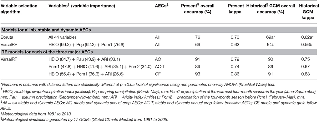
Table 2. Bioclimatic variables selected by Random Forest (RF) modeling of six and three agro-ecological classes (AECs).

The performance of reduced predictive Random Forest models for each of the three major AECs was superior to the all- and three-variable predictive models for the six AECs (Table 2). Cross validation performance statistics were greatest for the GF AEC where the overall accuracy for the Random Forest model using present data was 93%, followed closely by AC (91%) and AC-T (89%) (Table 2). In order of importance, the bioclimatic variables selected by Random Forest modeling of the AC AEC were (1) Holdridge evapotranspiration index, (2) autumn precipitation (Sep–Nov) (Pau), and (3) Aridity Index; for the AC-T AEC, (1) precipitation of the warmest 4-months, Jun–Sep (Pcm1), (2) Holdridge evapotranspiration index, (3) Aridity Index, and (4) precipitation of the 4-month season before Pcm1 (Feb–May) (Pcm2); and for the GF AEC, (1) Holdridge evapotranspiration index, (2) precipitation of the warmest 4-months, Jun–Sep, and (3) Aridity Index (Table 2). The performance metrics of the individual three variable predictive Random Forest models using historical GCM data did not deviate substantially from those using present meteorological data (Table 2).

Cross validation accuracy and reliability of Random Forest modeling for the six AECs were higher using all bioclimatic variables compared to the three variable Random Forest model (Table 3). Accuracy of a class is the percent of correctly classified pixels out of the actual number of pixels, whereas reliability of a class is the percent of correctly classified pixels out of the predicted number of pixels. Accuracy and reliability ranged from 48 to 89% and were generally greater for stable than dynamic AECs for the six AEC models. Irrespective of the Random Forest model used for all six AECs, predictive accuracy and reliability were highest for the stable GF class averaging 86% and lowest for the dynamic AC-T averaging 55% (Table 3). The accuracy and reliability of the Random Forest models for each of the three individual AECs were notably greater than that of the six AEC Random Forest models and averaged 89% for AC, 87% for AC-T, and 93% for GF (Table 3).

TABLE 3

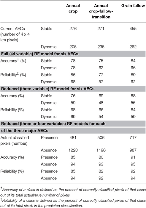
Table 3. Agro-ecological classes (AECs) in present time period and cross validation accuracy and reliability of full and reduced variable Random Forest (RF) models for six and three AECs.

Currently, stable AECs are 59% and dynamic AECs 41% of the total geographical distribution of dryland cropping systems (Table 3). The GF AEC currently has the largest area at 42%, followed by AC-T at 30% and AC at 28%. Spatially, dynamic AECs occur at the boundary of stable AECs (Figure 1). Here, non-parametric one-way ANOVA (Krushkal Wallis) showed significant differences in HBIO, Psp, and Pcm1 among all six AECs, except stable and dynamic AC-T (Table 4). HBIO means ranged from a low of 0.89 for dynamic AC-T to a high of 2.13 for stable GF. The stable GF had the lowest and dynamic AC-T the highest Psp and Pcm1. In addition, bioclimatic variability (CV) was higher for variables in dynamic compared to stable AECs (Table 4). Geospatial contours of HBIO, one of the most useful predictors, and current AECs showed similar patterns with division between AC and AC-T occurring about where HBIO was 1, while division between AC-T and GF occurred where HBIO was 1.5 (Figure 2).

TABLE 4

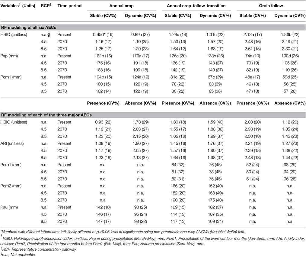
Table 4. Spatial average and coefficient of variation (CV%) of bioclimatic variables used with Random Forest (RF) models for present time period (1981–2010) and their future (2070) predictions under two representative concentration pathway (RCP- 4.5 and 8.5) scenarios derived from 17 global climate models.

FIGURE 2

Figure 2. Geo-spatial depiction of current Agro-ecological classes (AECs) and Holdridge Evapotranspiration index (HBIO) in present (1981–2010) and future climate scenario (2070, Representative Concentration Pathway, RCP-8.5).

Projected Changes in Bioclimatic Variables and Modeled Shifts in Current AECs

Increases in HBIO are projected under RCP 4.5 and 8.5 by 2070 (Table 4, Figure 2). Projected increases in Psp and declines in Pcm1 are anticipated across the iPNW. Both HBIO and ARI (different methods of calculating evapotranspiration and then dividing by precipitation) are predicted to increase and were selected as important for individual Random Forest modeling of the three major AECs, although HBIO showed greater predicted responses to climate change than ARI (Table 4). Increases in seasonal precipitation were predicted for AC and AC-T; Pcm2 increases were particularly important in AC-T, while Pau increased modestly for AC. In contrast, decreased Pcm1 was predicted for GF (Table 4).

A 46% decrease in area for dynamic AC and stable AC-T occurs if future climate scenarios of RCP 8.5 were imposed upon current production systems using the six AEC model (Table 5). Areas of stable AC and GF would decline more modestly (8 and 13%, respectively). In contrast, area would increase by 58 and 63%, respectively, for dynamic AC-T and GF. These results are depicted spatially in Figure 3 for 2070, RCP 8.5, and in comparison with present AECs (Figure 1), show dynamic AC-T and GF replacing dynamic AC and stable AC-T, GF, and AC. Coefficients of variation (CVs) of projected areas tended to be higher for dynamic compared to stable AECs and, with a few exceptions (stable AC-T, under RCP 4.5 and 8.5), generally increased as the twenty-first century progressed (Table 5).

TABLE 5

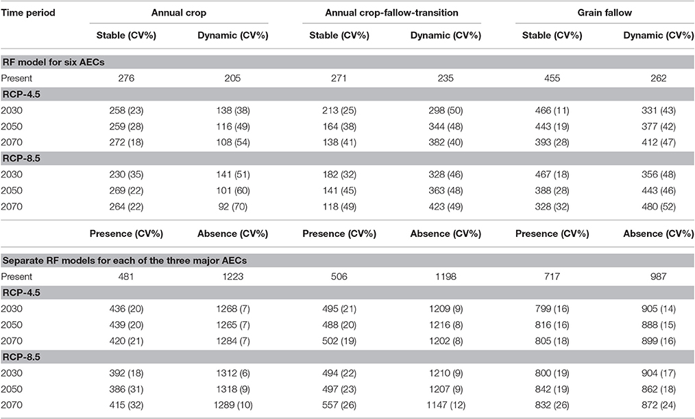
Table 5. Agro-ecological class (AEC) (number of 4 × 4 km pixels) for present time period and predicted number, average and coefficient of variation (CV%), under three future time periods and two representative concentration pathway (RCP-4.5 and 8.5) scenarios derived from 17 global climate models using Random Forest (RF) models for six and three AECs.

FIGURE 3

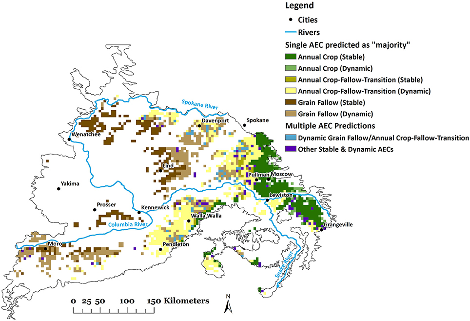
Figure 3. Projected geo-spatial distribution of six (stable and dynamic) agro-ecological classes (AECs) using combined Random Forest (RF) model of bioclimatic variables for six AECs under future climate scenario (2070, Representative Concentration Pathway, RCP-8.5).

In general, predictions for the main three AECs followed the same trends as the six AEC models, with the area under AC declining by 17%, AC-T increasing modestly (2%), and with more substantial area increases predicted for GF (15%) across all time periods of RCP 8.5 (Table 5). Here, CVs were generally lower under all future climate scenarios than for the six AEC models and did not have a strong tendency to increase with time. Spatial representations of the three main AEC Random Forest models for present day and a future scenario (2070 and RCP 8.5) generally indicate future areas under AC-T encroaching on present day AC while GF replaces AC-T (Figure 4).

FIGURE 4

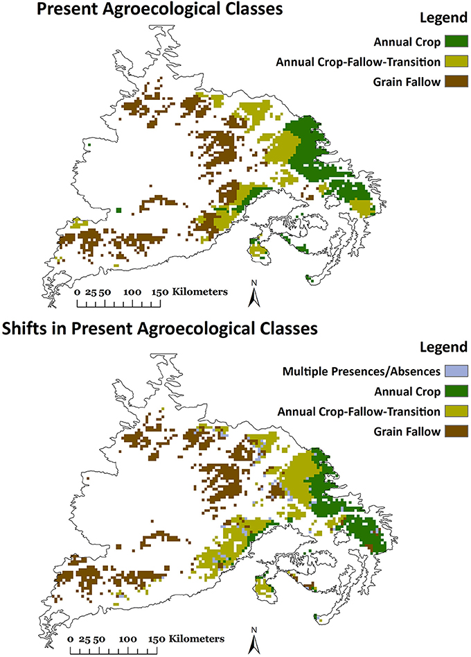
Figure 4. Projected geo-spatial distribution of three agro-ecological classes (AECs) using three individual Random Forest (RF) models of bioclimatic variables under future climate scenario (2070, Representative Concentration Pathway, RCP-8.5).

Discussion

Identification of Bioclimatic Predictors Useful for Discriminating among Current AECs

Our study emphasizes the use of bioclimatic variables as they contribute to the geographic distributions of species and are used in modeling species occurrence (Watling et al., 2012). The HBIO was identified as an important bioclimatic variable for AEC modeling and prediction of all six dryland AECs as well as each of the three main AECs. Computationally, HBIO is an annual average of monthly temperatures within a range of 0–30°C, which is multiplied by a constant (58.93; Holdridge, 1967) to give Holdridge evapotranspiration (ET) and then divided by annual precipitation. HBIO, an important variable in the Holdridge life zone classification, is defined as potential evapotranspiration ratio and as mentioned, is dependent on annual precipitation and annual bio-temperature, the other two important variables used in the classification. The Holdridge life zone classification model represents the relation between climate and vegetation pattern and has been used in climate change studies to investigate the impact of changing climate on species distributions in different ecosystems (Cameron and Scheel, 2001; Enquist, 2002). Values of HBIO < 1 indicates conditions of water sufficiency while HBIO > 1 suggests conditions of water insufficiency or deficiency for all plant and animal life forms (Savage, 2002). In the present study, the average HBIO of stable and dynamic AC AECs were < 1, while the remaining AECs, which all rely on fallow, had an HBIO > 1 (Table 4). Thus, empirically, HBIO emerged as an important bioclimatic variable for driving future changes in the extent and spatial distribution of AECs (Figures 1–3). Similarly, when considering 44 bioclimatic variables for each of the three major AECs, ET indices, namely HBIO, and ARI (Thornthwaite ET index; defined as ratio of Thornthwaite ET to annual precipitation), were identified as the most important driving variables for AEC modeling.

Our analyses do not consider potential beneficial effects of rising carbon dioxide (CO₂) levels on crop physiology including increases in water-use efficiency (WUE) and overall crop yield (Stöckle et al., 2010). Ramírez and Finnerty (1996) reported decreased potential evapotranspiration (PET) under elevated CO₂ conditions and a resultant increase in WUE. Therefore, HBIO, although a bio-temperature based estimate of PET, could decrease with greater levels of atmospheric CO₂, potentially compensating for increased HBIO resulting from warming. Significant increases in soil water availability (via reduced stomatal conductance) under elevated CO₂ levels (Lu et al., 2016) could also compensate for negative impacts reported here, particularly the use of annual fallow. Palmquist et al. (2016), however, projected increases in actual evapotranspiration, dry days, and large reductions in available soil water during summer due to climate change for the western U.S. including our study region. Here, potential ameliorating effects of elevated CO₂ levels were not considered. Nonetheless, offsets of positive influences of elevated CO₂ levels due to negative effects of increased temperatures on crop physiology and growth have also been reported (Reddy et al., 2002; Zavaleta et al., 2003). Ko et al. (2012) simulated that negative effects of increased temperature would dominate the positive effects of rising CO₂ levels on crop yields in dryland cereal-based rotations of the U.S. Central Great Plains. Consequently, a thorough understanding of positive and negative feedback mechanisms from climate-vegetation interactions including CO₂ levels remains elusive.

Previous studies have used annual precipitation as an important delineator to classify dryland cropping systems of the iPNW (Douglas et al., 1988, 1992). In the present study, however, spring precipitation (Psp) and precipitation during the warmest 4 months (Pcm1) were identified as more important empirical predictors of AECs than annual precipitation. From a crop production and soil water storage perspective, most of the annual precipitation occurs from November to May and is important for all dryland AECs of the iPNW (Schillinger et al., 2008). Also relevant, however, are quantities of spring and early summer rainfall (April–Jun) which coincide with anthesis and grain filling of winter and spring crops (Schillinger et al., 2008). Our study indicates that seasonal precipitation and temperature significantly contributed toward differentiating among AECs. These results have production relevance as decisions regarding spring flex-cropping options (whether to produce a spring crop or to fallow) would be based on winter precipitation rather than spring and summer rainfall. Consequently, more uncertainty would be associated with flex-cropping options, potentially promoting the use of annual fallow.

Predictive Capacity of AEC Models

There are numerous empirical approaches available to understand species distributions and analyze climate-species relations. In the present study, we used “Random Forest,” reported as a higher performance algorithm than other empirical approaches (Cutler et al., 2007; Schrag et al., 2008). Watling et al. (2012) did not report significant differences in prediction results using Random Forest with two different sets of variables (bioclimatic and monthly variables). Similarly, with our dataset, using Random Forest to predict current AECs resulted in comparable overall accuracy and kappa with cross validation on different sets of selected variables using two different variable selection methods. Elsewhere, the Random Forest approach has been successfully applied in various fields of research ranging from micro-array data analysis (Díaz-Uriarte and Alvarez de Andrés, 2006), hyper-spectral data analysis (Adam et al., 2012; Poona and Ismail, 2014), current species distribution studies, as well as in predicting distributions with changing future climate (Schrag et al., 2008; Watling et al., 2012; Langdon and Lawler, 2015). Random Forest belongs to the algorithmic modeling culture (Breiman, 2001) in statistical modeling where the data mechanisms are complex and not known. Therefore, Random Forest modeling results can be difficult to interpret and to identify underlying causal mechanisms. Nonetheless, Random Forest is gaining popularity over other empirical approaches for the following reasons: (1) it is non-parametric in nature and does not assume data distribution; (2) it is an ensemble classifier, its results are aggregated over the number of classification trees built/defined in the algorithm, and it avoids overfitting; and (3) the Random Forest algorithm is computationally more efficient and deals well with correlation and high-order interactions between input variables. For many datasets, utilizing Random Forest has proved to be highly accurate compared to other classifiers (Fernández-Delgado et al., 2014).

Performance of Random Forest as a predictive model was comparable with present meteorological as well as GCM data even with the reduction from 44 to 3 variables, which corroborated the high performance of the Random Forest algorithm (Table 2). The only limitation of using the reduced Random Forest model with three variables was that this might decrease the possible combinations which would otherwise be used by Random Forest to improve AEC classification accuracy. In predictive modeling, however, a less complex and parsimonious model that uses a few important and relevant variables with high explanatory power is easier to interpret than a model with many variables as long as overall accuracy is not too impaired and the less complex model is also able to capture the intricacies of the patterns and distributions modeled (Evans et al., 2011). In our research, the 44 (all variables) Random Forest model had greater accuracy and reliability than the three variable model, but there was little loss in performance by reducing the number of variables from 44 to 3 (Table 2). Therefore, we proceeded with the VarSelRF selection method to reduce model dimensionality as well as redundancy to facilitate interpretation (Murphy et al., 2010) for all subsequent Random Forest modeling of AECs, and also to avoid model overfitting, which occurs in complex models with increased model variance (Hastie et al., 2009; Table 3).

The range in accuracy and reliability for the three variable Random Forest model was much greater for stable than dynamic AECs (Table 3) indicating more uncertainty would occur in prediction of dynamic AECs when imposing future predicted changes in bioclimatic drivers. Contributing to the uncertainty of dynamic AEC prediction was the scattered spatial distribution (e.g., Thuiller et al., 2003) of dynamic AECs compared to the more compact distribution of stable AECs (Figures 1, 4). In turn, this contributed to higher CVs of selected bioclimatic variables within dynamic compared to stable AECs (Table 4). The relatively poor Random Forest model performance of the dynamic AECs led to modeling each of the three major AECs where stable and dynamic AECs were combined. Here, Random Forest modeling of the three major AECs separately improved overall Random Forest model accuracy from 69% to up to more than 93% (Table 2) and further identified the difficulty in using only bioclimatic variables in one Random Forest model to differentiate between stable and dynamic subclasses of major AECs. Thus, modeling three major AECs separately highlighted the role of bioclimatic variables and identified the need to include additional variables (e.g., soil, seasonal weather, and economic) if greater AEC model accuracy is required. The overall high accuracy (89–93%) of Random Forest modeling of the major AECs using only a few (3–4) bioclimatic variables was surprising as other socio-economic and biophysical factors contribute to current AEC outcomes (Figures 1, 4). It is important to recognize that the current AECs are derived from the Cropland datalayer (USDA-NASS, 2008–2015) and represents the land use/cover derived from the integration of biophysical and socio-economic factors. Our results, however, emphasize the fundamental importance of climatic variables in driving AEC outcomes and the potential for climate change to shape future AECs.

Regional Shifts in Current AECs under Future Climate Scenarios

It is important to recognize that our analyses simply impose future projections of relevant bioclimatic variables in modeling geo-spatial shifts of AECs under current production factors, including existing levels of atmospheric CO₂. The modeled changes in AECs indicate that cropping systems would be less stable and employ more annual fallow, thereby decreasing cropping system intensification. Currently, the GF AEC is the least flexible and diverse cropping system with few economic options with respect to crop choice, consisting primarily of winter wheat followed by annual fallow in short, 2-year rotations. Consequently, the GF AEC is the most vulnerable to extremes in weather or variations in markets, farm input costs, government policies and other sources of uncertainty. In contrast, the AC AEC has the most crop diversity and is relatively less vulnerable to future uncertainties, although improvements would be beneficial (Huggins et al., 2015).

Collectively, these results suggest a reduction in cropping intensity, potentially reduced yields (more fallow) and diversity, and increased area where cropping systems are less stable under climate change. These conclusions contrast sharply with results reported for the same region using process-oriented cropping system modeling that includes increasing future levels of CO₂ (Karimi et al., 2017; Stöckle et al., 2017). Here, crop yields are simulated to increase under the same climate change scenarios presented here with the conclusion that there will be less annual fallow. Challenges of biophysical modeling of cropping systems, however, include determining what factors determine the geospatial extent and location of a given cropping system. This challenge becomes more acute if cropping systems are projected to become more dynamic as in our study. Many factors other than crop yield, such as social-economic, yield stability and risk, disease, weed and pest pressure, are not fully integrated into crop models to determine the cropping system that would be used by producers. Here, projected yield increases may not necessarily result in less fallow and could actually be associated with more fallow to aid the stability of higher yields. Furthermore, if higher yields are associated with more area under annual fallow, then the overall crop yields of the region could decline. Our analyses use the cropping systems derived from the Cropland data-layer (USDA-NASS, 2008–2015) which are geo-spatial outcomes of producer decisions resulting from the integration of all contributing bio-physical and socio-economic factors. We contend, therefore, that future research will need to explore and develop production systems that promote intensification and diversification in the face of adverse climate change.

Relevance of AEC Shifts for Sustainable Agriculture

Processes affecting soil resources in dryland cropping systems of the iPNW include soil erosion through the action of wind, water, and tillage (McCool et al., 1998; Saxton et al., 2000; Sharratt et al., 2012), declining levels of soil organic matter (SOM; Rasmussen et al., 1989; Purakayastha et al., 2008), increasing soil acidification (Mahler et al., 1985; Brown et al., 2008), and decreasing soil biological activity and diversity (Elliott and Lynch, 1994). Currently, these degradation processes threaten the sustainability of the region's dryland cropping systems (McCool et al., 2001). Winter wheat following annual fallow combined with conventional tillage that leaves little protective surface crop or residue cover is particularly prone to soil erosion. Potential increases in HBIO and shifts toward more annual fallow due to climate change (Table 5) could increase the regional hazard of soil erosion. This could occur despite potential off-setting factors, such as increased crop biomass production due to CO₂ fertilization effects (Sharratt et al., 2015). Annual soil losses due to soil erosion by wind and water currently range from 1 to 50 Mg ha⁻¹ (Nagle and Ritchie, 2004; Kok et al., 2008; Sharratt et al., 2012). Rates of soil erosion below established USDA annual soil loss tolerance limits of 2.2–11.2 Mg ha⁻¹ (Renard et al., 1997) are likely required to meet agricultural sustainability goals (Montgomery, 2007) and could be achieved with continuous no-tillage under annual or perennial cropping systems that limit annual fallow (Huggins and Reganold, 2008; Huggins et al., 2014a).

Negative impacts of annual fallow on SOM, primarily due to decreased crop inputs, factors enhancing biological decomposition (e.g., tillage, water, and temperature), and increased vulnerability to soil erosion, are well-documented (Campbell et al., 1999; Liebig et al., 2006; Gan et al., 2012). Declining SOM associated with increasing regional climate ratios as projected by future climate change in the iPNW (Morrow et al., 2017) would further promote soil degradation processes by negatively impacting aggregate stability and microbial communities and their functions (Allen et al., 2011; Maestre et al., 2015). Annual fallow has been reported to adversely influence microbial biomass and activity (Steenwerth et al., 2002; Pankhurst et al., 2005) as well as obligatory symbiotic organisms such as arbuscular mycorrhizal fungi (Thompson, 1987; Pankhurst et al., 2005). The primary objective of annual fallow is to stabilize crop yields under conditions of low or widely varying precipitation (Greb et al., 1974). Annual fallow has been widely practiced across agricultural areas of the western United States and Prairie Provinces of Canada (Nielson and Calderon, 2011). In the iPNW, 2-year winter wheat–annual fallow rotations have dominated low annual precipitation areas with dryland cropping since the 1890s as this rotation is less risky and more profitable (Schillinger et al., 2006). Therefore, overcoming projected increases in annual fallow that would further threaten the regions agricultural sustainability under climate change will likely require diverse strategies that engage socio-economic as well as biophysical dimensions (Peterson et al., 1996; Pan et al., 2016; Maaz et al., in press).

Agricultural strategies to reduce or eliminate annual fallow and its adverse effects include: (1) conservation tillage practices; (2) intensification and diversification of cropping systems; (3) elimination of crop residue removal via residue burning or harvest; (4) use of soil amendments such as manures and bio-solids; and (5) policies that enhance the short-term economics of alternative crops and fallow replacement. Precipitation-use efficiency, under cropping systems with annual fallow, ranges from 10 to 40% (Peterson et al., 1996; Farahani et al., 1998). Reviewing the literature, Hatfield et al. (2001) concluded that increases in WUE of 25–40% could be achieved through conservation tillage and cropping system intensification in semiarid environments. Peterson et al. (1996), however, stated that despite improvements in WUE or environmental factors, adoption of intensified cropping systems depended more on favorable economic outcomes and government programs. In the iPNW, various alternative crop and opportunity (flex) crop options have been explored such as canola (Pan et al., 2016; Maaz et al., in press), facultative wheat (Bewick et al., 2008), and fallow replacement with no-till spring wheat (Thorne et al., 2003). Maaz et al. (in press) concluded, however, given the economic competitiveness of wheat in the iPNW, that (1) economic approaches should be broadened to allow crop rotational rather than single commodity assessments; (2) crop insurance policies should consider more support of whole farm risk management options; and (3) additional multi-commodity groups with an interest in market-driven crop diversification should be established.

Conclusions

Bioclimatic variables were useful for discriminating among iPNW AECs using Random Forest models. In particular, potential evapotranspiration based indices proved to be more relevant predictors of present iPNW AECs than annual precipitation which is commonly used to describe agricultural zones. Super-imposing future climate scenarios onto current agricultural production systems resulted in significant geospatial shifts in AECs. Dynamic and fallow-based AECs increased in area while stable AECs and annual cropping AECs decreased. Increasing annual fallow is counter to cropping system objectives of increasing intensification, diversification, and productivity. Furthermore, more annual fallow would aggravate soil degradation processes by increasing vulnerability to soil erosion and adversely impacting soil organic matter and biological activity. Our model results do not integrate important future influences including technological and scientific advances, changing agricultural markets, and economies and rising atmospheric CO₂ levels. Integrative, transdisciplinary research that includes genetic, environmental, management, and social-economic dimensions will be required if sustainable agricultural systems are to be developed to address future uncertainties including climate change.

Author Contributions

DH, RR, JA, CS, and JR have served on HK's Ph.D. research committee and aided the development of research objectives, methods, and discussion. HK: Worked with the climate and AEC data in ArcGIS and R, developed methods with the help of all committee members to run the empirical analysis. DH: Corresponding author and PI of the project, has made substantial contribution to this study, provided his time in discussion, advising, guiding, and funding to conduct the study and as well as provided immense help in organizing, writing and editing the manuscript. RR has made significant contribution in providing guidance on all the ArcGIS methods applied in this study, provided his time in discussion and answering queries related to ArcGIS. JA has made good amount of contribution by helping answering queries related to accessing climate data during the course of study and provided helpful edits on the manuscript. CS: Provided suggestions during the course of the study which were helpful in improving the study and as well as suggestions on the manuscript. JR: Provided suggestions during the course of the study which were helpful in improving the study and as well as suggestions and edits on the manuscript.

Funding

This study is part of the project “Regional Approaches to Climate Change for Pacific Northwest Agriculture,” funded through award #2011-68002-30191 from the USDA-National Institute for Food and Agriculture.

Conflict of Interest Statement

The handling Editor declared a shared affiliation, though no other collaboration, with one of the authors JA and states that the process nevertheless met the standards of a fair and objective review.

The authors declare that the research was conducted in the absence of any commercial or financial relationships that could be construed as a potential conflict of interest.

References

Abatzoglou, J. T. (2013). Development of gridded surface meteorological data for ecological applications and modelling. Int. J. Climatol. 33, 121–131. doi: 10.1002/joc.3413

CrossRef Full Text | Google Scholar

Abatzoglou, J. T., and Brown, T. J. (2012). A comparison of statistical downscaling methods suited for wildfire applications. Int. J. Climatol. 32, 772–780. doi: 10.1002/joc.2312

CrossRef Full Text | Google Scholar

Adam, E. M., Mutanga, O., Rugege, D., and Ismail, R. (2012). Discriminating the papyrus vegetation (Cyperus papyrus L.) and its co-existent species using random forest and hyperspectral data resampled to HYMAP. Int. J. Remote Sen. 33, 552–569. doi: 10.1080/01431161.2010.543182

CrossRef Full Text | Google Scholar

Allen, D. E., Singh, B. P., and Dalal, R. C. (2011). “Soil health indicators under climate change: a review of current knowledge” in Soil Health and Climate Change, eds B. P. Singh, A. L. Cowie, and K. Y. Chan (Berlin; Heidelberg: Springer), 25–45.

Google Scholar

Bewick, L. S., Young, F. L., Alldredge, J. R., and Young, D. L. (2008). Agronomics and economics of no-till facultative wheat in the Pacific Northwest. Crop. Prot. 27, 932–942. doi: 10.1016/j.cropro.2007.11.013

CrossRef Full Text | Google Scholar

Breiman, L. (2001). Statistical modeling: the two cultures. Statist. Sci. 16, 199–231. doi: 10.1214/ss/1009213726

CrossRef Full Text | Google Scholar

Brown, T. T., Koenig, R. T., Huggins, D. R., Harsh, J. B., and Rossi, R. E. (2008). Lime effects on soil acidity, crop yield, and aluminum chemistry in direct-seeded cropping systems. Soil Sci. Soc. Am. J. 72, 634–640. doi: 10.2136/sssaj2007.0061

CrossRef Full Text | Google Scholar

Cameron, G. N., and Scheel, D. (2001). Getting warmer: effect of global climate change on distribution of rodents in texas. J. Mammal. 82, 652–680. doi: 10.1644/1545-1542(2001)082<0652:GWEOGC>2.0.CO;2

CrossRef Full Text | Google Scholar

Campbell, C. A., Biederbeck, V. O., McConkey, B. G., Curtin, D., and Zentner, R. P. (1999). Soil organic matter quality as influenced by tillage and fallow frequency in a silt loam in southwestern Saskatchewan. Soil Biol. Biochem. 31, 1–7. doi: 10.1016/S0038-0717(97)00212-5

CrossRef Full Text | Google Scholar

Chang, T., Hansen, A. J., and Piekielek, N. (2014). Patterns and variability of projected bioclimatic habitat for Pinus albicaulis in the greater yellowstone area. PLoS ONE 9:e111669. doi: 10.1371/journal.pone.0111669

PubMed Abstract | CrossRef Full Text | Google Scholar

Chen, I.-C., Hill, J. K., Ohlemüller, R., Roy, D. B., and Thomas, C. D. (2011). Rapid range shifts of species associated with high levels of climate warming. Science 333, 1024. doi: 10.1126/science.1206432

PubMed Abstract | CrossRef Full Text | Google Scholar

Clark, J., Wang, Y., and August, P. V. (2014). Assessing current and projected suitable habitats for tree-of-heaven along the Appalachian Trail. Philos. Trans. R. Soc. Lond. B Biol. Sci. 369:20130192. doi: 10.1098/rstb.2013.0192

PubMed Abstract | CrossRef Full Text | Google Scholar

Cutler, D. R., Edwards, T. C., Beard, K. H., Cutler, A., Hess, K. T., Gibson, J., et al. (2007). Random forests for classification in ecology. Ecology 88, 2783–2792. doi: 10.1890/07-0539.1

PubMed Abstract | CrossRef Full Text | Google Scholar

de Mendiburu, F. (2015). Agricolae: Statistical Procedures for Agricultural Research. R package version 1.2-3. Available online at: http://CRAN.R-project.org/package=agricolae

Diaz-Uriarte, R. (2014). varSelRF: Variable Selection using Random Forests. R package version 0.7-5. Available online at: http://CRAN.R-project.org/package=varSelRF

Díaz-Uriarte, R., and Alvarez de Andrés, S. (2006). Gene selection and classification of microarray data using random forest. BMC Bioinform. 7:3. doi: 10.1186/1471-2105-7-3

PubMed Abstract | CrossRef Full Text | Google Scholar

Douglas, C. L. Jr., Rickman, R. W., Klepper, B. L., and Zuzel, J. F. (1992). Agroclimatic zones for dryland winter wheat producing areas of Idaho, Washington and Oregon. Northwest Sci. 66, 26–34.

Google Scholar

Douglas, C. L. Jr., Rickman, R. W., Zuzel, J. F., and Klepper, B. L. (1988). Criteria for delineation of agronomic zones in the Pacific North-west. J. Soil Water Conserv. 43, 415–418.

Google Scholar

Elliott, L. F., and Lynch, J. M. (1994). “Biodiversity and soil resilience,” in Soil Resilience and Sustainable Land Use, eds D. J. Greenland, and I. Szaboles (Wallingford, UK: CAB International), 353–364.

Google Scholar

Enquist, C. A. F. (2002). Predicted regional impacts of climate change on the geographical distribution and diversity of tropical forests in Costa Rica. J. Biogeogr. 29, 519–534. doi: 10.1046/j.1365-2699.2002.00695.x

CrossRef Full Text | Google Scholar

ESRI (2011). ArcGIS Desktop: 10.3.1. Redlands, CA: ESRI. Available online at: http://www.esri.com/index.html

Estes, L. D., Beukes, H., Bradley, B. A., Debats, S. R., Oppenheimer, M., Ruane, A. C., et al. (2013). Projected climate impacts to South African maize and wheat production in 2055: a comparison of empirical and mechanistic modeling approaches. Global Change Biol. 19, 3762–3774. doi: 10.1111/gcb.12325

PubMed Abstract | CrossRef Full Text | Google Scholar

Evangelista, P., Young, N., and Burnett, J. (2013). How will climate change spatially affect agriculture production in Ethiopia? Case studies of important cereal crops. Clim. Change 119, 855–873. doi: 10.1007/s10584-013-0776-6

CrossRef Full Text | Google Scholar

Evans, J. S., Murphy, M. A., Holden, Z. A., and Cushman, S. A. (2011). “Modeling species distribution and change using random forest,” in Predictive Species and Habitat Modeling in Landscape Ecology, eds C. A. Drew, Y. F. Wiersma, and F. Huettmann (New York, NY: Springer), 139–159.

Google Scholar

Farahani, H. J., Peterson, G. A., Westfall, D. G., Sherrod, L. A., and Ahuja, L. R. (1998). Soil water storage in dryland cropping systems: the significance of cropping intensification. Soil Sci. Soc. Am. J. 62, 984–991. doi: 10.2136/sssaj1998.03615995006200040020x

CrossRef Full Text | Google Scholar

Fernández-Delgado, M., Cernadas, E., Barro, S., and Amorim, D. (2014). Do we need hundreds of classifiers to solve real world classification problems? J. Mach. Learn. Res. 15, 3133–3181.

Google Scholar

Fortino, V., Kinaret, P., Fyhrquist, N., Alenius, H., and Greco, D. (2014). A robust and accurate method for feature selection and prioritization from multi-class OMICs data. PLoS ONE 9:e107801. doi: 10.1371/journal.pone.0107801

PubMed Abstract | CrossRef Full Text | Google Scholar

Gan, Y., Liang, C., Campbell, C. A., Zentner, R. P., Lemke, R. L., Wang, H., et al. (2012). Carbon footprint of spring wheat in response to fallow frequency and soil carbon changes over 25 years on the semiarid Canadian prairie. Eur. J. Agron. 43, 175–184. doi: 10.1016/j.eja.2012.07.004

CrossRef Full Text | Google Scholar

Gonzalez, P. (2001). Desertification and a shift of forest species in the West African Sahel. Clim. Res. 17, 217–228. doi: 10.3354/cr017217

CrossRef Full Text | Google Scholar

Greb, B. W., Smika, D. E., Woodruff, N. P., and Whitfield, C. J. (1974). “Summer fallow in the central Great Plains,” in USDA-ARS Conserv. Res. Rep. No. 17. (Washington, DC: U.S. Gov. Print. Office), 51–85.

Google Scholar

Guo, P., Zhang, Q., Zhu, Z., Huang, Z., and Li, K. (2014). Mining gene expression data of multiple sclerosis. PLoS ONE 9:e100052. doi: 10.1371/journal.pone.0100052

PubMed Abstract | CrossRef Full Text | Google Scholar

Hastie, T., Tibshirani, R., and Friedman, J. (2009). The Elements of Statistical Learning:Data Mining, Inference, and Prediction, 2nd Edn. New York, NY: Springer.

Hatfield, J. L., Sauer, T. J., and Prueger, J. H. (2001). Managing soils to achieve greater water use efficiency. Agron. J. 93, 271–280. doi: 10.2134/agronj2001.932271x

CrossRef Full Text | Google Scholar

Holdridge, L. R. (1967). Life Zone Ecology. San Jose, CA: Tropical Science Center.

Google Scholar

Huggins, D. R., and Reganold, J. P. (2008). No-till: the quiet revolution. Sci. Am. 299, 70–77. doi: 10.1038/scientificamerican0708-70

PubMed Abstract | CrossRef Full Text | Google Scholar

Huggins, D. R., Kruger, C. E., Painter, K. M., and Uberuaga, D. P. (2014a). Site-specific trade-offs of harvesting cereal residues as biofuel feedstocks in dryland annual cropping systems of the pacific northwest, U.S.A. BioEnergy Res. 7, 598–608. doi: 10.1007/s12155-014-9438-4

CrossRef Full Text | Google Scholar

Huggins, D. R., Rupp, R., Kaur, H., and Eigenbrode, S. (2014b). “Defining agroecological classes for assessing land use dynamics,” in Regional Approaches to Climate Change for Pacific Northwest Agriculture, eds K. Borrelli, D. Daley-Laursen, S. Eigenbrode, B. Mahler, and B. Stokes (Moscow: University of Idaho), 4–7.

Google Scholar

Huggins, D., Pan, W., Schillinger, W., Young, F., Machado, S., and Painter, K. (2015). “Crop diversity and intensity in Pacific Northwest dryland cropping systems,” in Regional Approaches to Climate Change for Pacific Northwest, eds K. Borrelli, D. Daley-Laursen, S. Eigenbrode, B. Mahler, and R. Pepper (Moscow: University of Idaho), 38–41.

Karimi, T., Stöckle, C. O., Higgins, S., Nelson, R. L., and Huggins, D. R. (2017). Projected dryland cropping system shifts in the Pacific Northwest in response to climate change. Front. Ecol. Evol. 5:20. doi: 10.3389/fevo.2017.00020

CrossRef Full Text | Google Scholar

Ko, J., Ahuja, L. R., Saseendran, S. A., Green, T. R., Ma, L., Nielsen, D. C., et al. (2012). Climate change impacts on dryland cropping systems in the Central Great Plains, U. S. A. Clim. Change 111, 445–472. doi: 10.1007/s10584-011-0175-9

CrossRef Full Text | Google Scholar

Kok, H., Papendick, R. I., and Saxton, K. E. (2008). STEEP: impact of long-term conservation farming research and education in Pacific Northwest wheatlands. J. Soil Water Conserv. 64, 253–264. doi: 10.2489/jswc.64.4.253

CrossRef Full Text | Google Scholar

Kuhn, M. (2015). Caret: Classification and Regression Training. R Package, v515. Available online at: http://cran.r-project.org/web/packages/caret/

Kumar, S., Merwade, V., Rao, P. S. C., and Pijanowski, B. C. (2013). Characterizing long-term land use/cover change in the united states from 1850 to 2000 using a nonlinear bi-analytical model. Ambio 42, 285–297. doi: 10.1007/s13280-012-0354-6

PubMed Abstract | CrossRef Full Text | Google Scholar

Kursa, M. B., and Rudnicki, W. R. (2010). Feature selection with the Boruta package. J. Stat. Softw. 36, 1–13. doi: 10.18637/jss.v036.i11

CrossRef Full Text | Google Scholar

Langdon, J. G. R., and Lawler, J. J. (2015). Assessing the impacts of projected climate change on biodiversity in the protected areas of western North America. Ecosphere 6, 1–14. doi: 10.1890/ES14-00400.1

CrossRef Full Text | Google Scholar

Lawler, J. J., Shafer, S. L., White, D., Kareiva, P., Maurer, E. P., Blaustein, A. R., et al. (2009). Projected climate-induced faunal change in the Western Hemisphere. Ecology 90, 588–597. doi: 10.1890/08-0823.1

PubMed Abstract | CrossRef Full Text | Google Scholar

Liebig, M., Carpenter-Boggs, L., Johnson, J. M. F., Wright, S., and Barbour, N. (2006). Cropping system effects on soil biological characteristics in the Great Plains. Renew. Agr. Food Syst. 21, 36–48. doi: 10.1079/RAF2005124

CrossRef Full Text | Google Scholar

Lu, X., Wang, L., and McCabe, M. F. (2016). Elevated CO₂ as a driver of global dryland greening. Sci. Rep. 6:20716. doi: 10.1038/srep20716

CrossRef Full Text | Google Scholar

Maaz, T., Wulfhorst, J. D., McCracken, V., Kirkegaard, J., Huggins, D. R., Roth, I., et al. (in press). Economic, policy, social trends challenges of introducing oilseed pulse crops into dryland wheat rotations. Agric. Ecosyst. Environ. doi: 10.1016/j.agee.2017.03.018

CrossRef Full Text | Google Scholar

Maestre, F. T., Delgado-Baquerizo, M., Jeffries, T. C., Eldridge, D. J., Ochoa, V., Gozalo, B., et al. (2015). Increasing aridity reduces soil microbial diversity and abundance in global drylands. Proc. Natl. Acad. Sci. U.S.A. 112, 15684–15689. doi: 10.1073/pnas.1516684112

PubMed Abstract | CrossRef Full Text | Google Scholar

Mahler, R. L., Halvorson, A. R., and Koehler, F. E. (1985). Long-term acidification of farmland in northern Idaho and Eastern Washington. Commun. Soil Sci. Plan. 16, 83–95. doi: 10.1080/00103628509367589

CrossRef Full Text | Google Scholar

McCool, D. K., Huggins, D. R., Saxton, K. E., and Kennedy, A. C. (2001). “Factors affecting agricultural sustainability in the Pacific Northwest, USA: an overview,” in Sustaining the Global Farm, 255-260, Selected Papers from the 10th International Soil Conservation Organization Meeting held May 24–29, 1999, eds D. E. Stott, R. H. Mohtar, and G. C. Steinhardt (West Lafayette: Purdue University and the USDA-ARS National Soil Erosion Research Laboratory).

Google Scholar

McCool, D. K., Montgomery, J. A., Busacca, A. J., and Frazier, B. E. (1998). “Soil degradation by tillage movement,” in International Soil Conservation Organization Conference Proceedings: Advances in GeoEcology (West Lafayette: Catena-Verlag), 327–332.

Monadjem, A., Virani, M. Z., Jackson, C., and Reside, A. (2013). Rapid decline and shift in the future distribution predicted for the endangered Sokoke Scops Owl Otus ireneae due to climate change. Bird Conserv. Int. 23, 247–258. doi: 10.1017/S0959270912000330

CrossRef Full Text | Google Scholar

Montgomery, D. R. (2007). Soil erosion and agricultural sustainability. Proc. Natl. Acad. Sci. U.S.A. 104, 13268–13272. doi: 10.1073/pnas.0611508104

PubMed Abstract | CrossRef Full Text | Google Scholar

Morrow, J. G., Huggins, D. R., and Reganold, J. P. (2017). Climate change predicted to negatively influence surface soil organic matter of dryland cropping systems in the inland Pacific Northwest, U. S. A. Front. Ecol. Evol. 5:10. doi: 10.3389/fevo.2017.00010

CrossRef Full Text | Google Scholar

Murphy, M. A., Evans, J. S., and Storfer, A. (2010). Quantifying Bufo boreas connectivity in Yellowstone National Park with landscape genetics. Ecology 91, 252–261. doi: 10.1890/08-0879.1

PubMed Abstract | CrossRef Full Text | Google Scholar

Nagle, G. N., and Ritchie, J. C. (2004). Wheat field erosion rates and channel bottom sediment sources in an intensively cropped northeastern Oregon drainage basin. Land Degrad. Dev. 15, 15–26. doi: 10.1002/ldr.587

CrossRef Full Text | Google Scholar

Nielson, D. C., and Calderon, F. J. (2011). “Fallow effects on soil,” in Soil Management: Building a Stable Base for Agriculture, eds J. L. Hatfield and T. J. Sauer (Madison, WI: ACSESS Publications: Soil Science Society of America), 287–300.

Omernik, J., and Griffith, G. (2014). Ecoregions of the conterminous united states: evolution of a hierarchical spatial framework. Environ. Manag. 54, 1249–1266. doi: 10.1007/s00267-014-0364-1

PubMed Abstract | CrossRef Full Text | Google Scholar

Ovalle-Rivera, O., Läderach, P., Bunn, C., Obersteiner, M., and Schroth, G. (2015). Projected Shifts in Coffea arabica Suitability among major global producing regions due to climate change. PLoS ONE 10:e0124155. doi: 10.1371/journal.pone.0124155

PubMed Abstract | CrossRef Full Text | Google Scholar

Palmquist, K. A., Schlaepfer, D. R., Bradford, J. B., and Lauenroth, W. K. (2016). Spatial and ecological variation in dryland ecohydrological responses to climate change: implications for management. Ecosphere 7:e01590. doi: 10.1002/ecs2.1590

CrossRef Full Text | Google Scholar

Pan, W. L., Young, F. L., Maaz, T. M., and Huggins, D. R. (2016). Canola integration into semi-arid wheat cropping systems of the inland Pacific Northwestern, U.S.A. Crop Pasture Sci. 67, 253–265. doi: 10.1071/CP15217

CrossRef Full Text | Google Scholar

Pankhurst, C. E., Stirling, G. R., Magarey, R. C., Blair, B. L., Holt, J. A., Bell, M. J., et al. (2005). Quantification of the effects of rotation breaks on soil biological properties and their impact on yield decline in sugarcane. Soil Biol. Biochem. 37, 1121–1130. doi: 10.1016/j.soilbio.2004.11.011

CrossRef Full Text | Google Scholar

Pauli, H., Gottfried, M., Reiter, K., Klettner, C., and Grabherr, G. (2007). Signals of range expansions and contractions of vascular plants in the high Alps: observations (1994–2004) at the GLORIA* master site Schrankogel, Tyrol, Austria. Global Change Biol. 13, 147–156. doi: 10.1111/j.1365-2486.2006.01282.x

CrossRef Full Text | Google Scholar

Peinado, M., Díaz, G., Delgadillo, J., Ocaña-Peinado, F. M., Macías, M. A., Aguirre, J. L., et al. (2012). Bioclimate-vegetation interrelations along the pacific rim of North America. Am. J. Plant Sci. 3, 1430–1450. doi: 10.4236/ajps.2012.310173

CrossRef Full Text | Google Scholar

Peterson, G. A., Schlegel, A. J., Tanaka, D. L., and Jones, O. R. (1996). Precipitation use efficiency as affected by cropping and tillage systems. J. Prod. Agric. 8, 180–186. doi: 10.2134/jpa1996.0180

CrossRef Full Text | Google Scholar

Pompe, S., Hanspach, J., Badeck, F., Klotz, S., Thuiller, W., and Kühn, I. (2008). Climate and land use change impacts on plant distributions in Germany. Biol. Lett. 4, 564–567. doi: 10.1098/rsbl.2008.0231

PubMed Abstract | CrossRef Full Text | Google Scholar

Poona, N. K., and Ismail, R. (2014). Using boruta-selected spectroscopic wavebands for the asymptomatic detection of Fusarium circinatum stress. IEEE J. Sel. Topics Appl. Earth Observ. in Remote Sens. 7, 3764–3772. doi: 10.1109/JSTARS.2014.2329763

CrossRef Full Text | Google Scholar

Purakayastha, T. J., Rudrappa, L., Singh, D., Swarup, A., and Bhadraray, S. (2008). Long-term impact of fertilizers on soil organic carbon pools and sequestration rates in maize–wheat–cowpea cropping system. Geoderma 144, 370–378. doi: 10.1016/j.geoderma.2007.12.006

CrossRef Full Text | Google Scholar

R Core Team (2015). R: A Language and Environment for Statistical Computing. Vienna: R Foundation for Statistical Computing. Available online at: https://www.R-project.org/

Ramírez, J. A., and Finnerty, B. (1996). CO₂ and temperature effects on evapotranspiration and irrigated agriculture. ASCE J. Irrig. Drain. Eng. 122, 155–163. doi: 10.1061/(ASCE)0733-9437(1996)122:3(155)

CrossRef Full Text | Google Scholar

Rasmussen, P. E., Collins, H. P., and Smiley, R. W. (1989). “Long-term management effects on soil productivity and crop yield in semi-arid regions of Eastern Oregon,” in Agricultural Experiment Station, Bulletin No. 675 (Pendleton, OR: Oregon State University).

Google Scholar

Rasztovits, E., Moricz, N., Berki, I., Potzelsberger, E., and Matyas, C. (2012). Evaluating the performance of stochastic distribution models for European beech at low-elevation xeric limits. Q. J. Hungarian Meteorol. Serv. 116, 173–194.

Reddy, K. R., Doma, P. R., Mearns, L. O., Boone, M. Y. L., Hodges, H. F., Richardson, A. G., et al. (2002). Simulating the impacts of climate change on cotton production in the Mississippi Delta. Clim Res. 22, 271–281. doi: 10.3354/cr022271

CrossRef Full Text | Google Scholar

Ren, Z., Wang, D., Ma, A., Hwang, J., Bennett, A., Sturrock, H. J. W., et al. (2016). Predicting malaria vector distribution under climate change scenarios in China: challenges for malaria elimination. Sci. Rep. 6:20604. doi: 10.1038/srep20604

PubMed Abstract | CrossRef Full Text | Google Scholar

Renard, K. G., Foster, G. R., Weesies, G. A., McCool, D. K., and Yoder, D. C. (1997). Predicting Soil Erosion by Water: A Guide to Conservation Planning with the Revised Universal Soil Loss Equation (RUSLE). Washington, DC: US Government Printing Office, USDA.

Google Scholar

Rupp, D. E., Abatzoglou, J. T., Hegewisch, K. C., and Mote, P. W. (2013). Evaluation of CMIP5 20th century climate simulations for the Pacific Northwest, U. S. A. J. Geophys. Res. Atmos. 118, 10884–10906. doi: 10.1002/jgrd.50843

CrossRef Full Text | Google Scholar

Savage, J. M. (2002). The Amphibians and Reptiles of Costa Rica: A Herpetofauna between Two Continents, between Two Seas. Chicago, IL; London: University of Chicago Press.

Google Scholar

Saxton, K. D., Chandler, L., Stetler, B., Lamb, C., Claiborn, B., and Lee, H. (2000). Wind erosion and fugitive dust fluxes on agricultural lands in the pacific northwest. T. ASAE 43, 631–640. doi: 10.13031/2013.2743

CrossRef Full Text | Google Scholar

Schillinger, W. F., Papendick, R. I., Guy, S. O., Rasmussen, P. E., and van Kessel, C. (2006). “Dryland Cropping in the Western United States,” in Agronomy Monograph No. 23, Dryland Agriculture, eds G. A. Peterson, P. W. Unger, and W. A. Payne (Madison, WI: American Society of Agronomy, Crop Science Society of America, Soil Science Society of America), 365–393.

Google Scholar

Schillinger, W. F., Schofstoll, S. E., and Alldredge, J. R. (2008). Available water and wheat grain yield relations in a Mediterranean climate. Field Crop. Res. 109, 45–49. doi: 10.1016/j.fcr.2008.06.008

CrossRef Full Text | Google Scholar

Schrag, A. M., Bunn, A. G., and Graumlich, L. J. (2008). Influence of bioclimatic variables on tree-line conifer distribution in the Greater Yellowstone Ecosystem: implications for species of conservation concern. J. Biogeogr. 35, 698–710. doi: 10.1111/j.1365-2699.2007.01815.x

CrossRef Full Text | Google Scholar

Sharratt, B. S., Tatarko, J., Abatzoglou, J. T., Fox, F. A., and Huggins, D. (2015). Implications of climate change on wind erosion of agricultural lands in the Columbia plateau. Weather Clim. Extremes 10, 20–31. doi: 10.1016/j.wace.2015.06.001

CrossRef Full Text | Google Scholar

Sharratt, B. S., Wendling, L., and Feng, G. (2012). Surface characteristics of a wind blown soil altered by tillage intensity during summer fallow. Aeol. Res. 5, 1–7. doi: 10.1016/j.aeolia.2012.02.002

CrossRef Full Text

Steenwerth, K. L., Jackson, L. E., Calderón, F. J., Stromberg, M. R., and Scow, K. M. (2002). Soil microbial community composition and land use history in cultivated and grassland ecosystems of coastal California. Soil Biol. Biochem. 34, 1599–1611. doi: 10.1016/S0038-0717(02)00144-X

CrossRef Full Text | Google Scholar

Stöckle, C. O., Higgins, S., Nelson, R., Abatzoglou, J., Huggins, D., Pan, W., et al. (2017). Evaluating opportunities for an increased role of winter crops as adaptation to climate change in dryland cropping systems of the U.S. Inland Pacific Northwest. Clim. Change. 1–15 doi: 10.1007/s10584-017-1950-z

CrossRef Full Text

Stöckle, C. O., Nelson, R. L., Higgins, S., Brunner, J., Grove, G., Boydston, R., et al. (2010). Assessment of climate change impact on Eastern Washington agriculture. Clim. Change 102, 77–102. doi: 10.1007/s10584-010-9851-4

CrossRef Full Text | Google Scholar

Taylor, K. E., Stouffer, R. J., and Meehl, G. A. (2012). An overview of CMIP5 and the experiment design. Bull. Am. Meteor. Soc. 93, 485–498. doi: 10.1175/BAMS-D-11-00094.1

CrossRef Full Text | Google Scholar

Thompson, J. P. (1987). Decline of vesicular-arbuscular mycorrhizae in long fallow disorder of field crops and its expression in phosphorus deficiency of sunflower. Aust. J. Agric. Res. 38, 847–867. doi: 10.1071/AR9870847

CrossRef Full Text | Google Scholar

Thorne, M. E., Young, F. L., Pan, W. L., Bafus, R., and Alldredge, J. R. (2003). No-till spring cereal cropping systems reduce wind erosion susceptibility in the wheat/fallow region of the Pacific Northwest. J. Soil Water Conserv. 58, 250–257.

Google Scholar

Thuiller, W., Araújo, M. B., and Lavorel, S. (2003). Generalized models vs. classification tree analysis: predicting spatial distributions of plant species at different scales. J. Veg. Sci. 14, 669–680. doi: 10.1111/j.1654-1103.2003.tb02199.x

CrossRef Full Text | Google Scholar

USDA-NASS (2008–2015). US Department of Agriculture National Agricultural Statistics Service Cropland Data Layer published during 2008 to 2015. Available online at: https://nassgeodata.gmu.edu/CropScape/

USDA-NRCS (2006). United States Department of Agriculture, Natural Resources Conservation Service: Land Resource Regions and Major Land Resource Areas of the United States, the Caribbean, and the Pacific Basin, U.S. Department of Agriculture Handbook, 296.

Watling, J. I., Roma-ach, S. S., Bucklin, D. N., Speroterra, C., Brandt, L. A., Pearlstine, L. G., et al. (2012). Do bioclimate variables improve performance of climate envelope models? Ecol. Model. 246, 79–85. doi: 10.1016/j.ecolmodel.2012.07.018

CrossRef Full Text | Google Scholar

Wilson, R. J., Gutiérrez, D., Gutiérrez, J., Martínez, D., Agudo, R., and Monserrat, V. J. (2005). Changes to the elevational limits and extent of species ranges associated with climate change. Ecol. Lett. 8, 1138–1146. doi: 10.1111/j.1461-0248.2005.00824.x

PubMed Abstract | CrossRef Full Text | Google Scholar

Zavaleta, E. S., Thomas, B. D., Chiariello, N. R., Asner, G. P., Shaw, M. R., and Field, C. B. (2003). Plants reverse warming effect on ecosystem water balance. Proc. Natl. Acad. Sci. U.S.A. 100, 9892–9893. doi: 10.1073/pnas.1732012100

PubMed Abstract | CrossRef Full Text | Google Scholar

Zhang, G., Dong, J., Zhou, C., Xu, X., Wang, M., Ouyang, H., et al. (2013). Increasing cropping intensity in response to climate warming in Tibetan Plateau, China. Field Crop. Res. 142, 36–46. doi: 10.1016/j.fcr.2012.11.021

CrossRef Full Text | Google Scholar