A Primer on High-Throughput Computing for Genomic Selection

High-throughput computing (HTC) uses computer clusters to solve advanced computational problems, with the goal of accomplishing high-throughput over relatively long periods of time. In genomic selection, for example, a set of markers covering the entire genome is used to train a model based on known data, and the resulting model is used to predict the genetic merit of selection candidates. Sophisticated models are very computationally demanding and, with several traits to be evaluated sequentially, computing time is long, and output is low. In this paper, we present scenarios and basic principles of how HTC can be used in genomic selection, implemented using various techniques from simple batch processing to pipelining in distributed computer clusters. Various scripting languages, such as shell scripting, Perl, and R, are also very useful to devise pipelines. By pipelining, we can reduce total computing time and consequently increase throughput. In comparison to the traditional data processing pipeline residing on the central processors, performing general-purpose computation on a graphics processing unit provide a new-generation approach to massive parallel computing in genomic selection. While the concept of HTC may still be new to many researchers in animal breeding, plant breeding, and genetics, HTC infrastructures have already been built in many institutions, such as the University of Wisconsin–Madison, which can be leveraged for genomic selection, in terms of central processing unit capacity, network connectivity, storage availability, and middleware connectivity. Exploring existing HTC infrastructures as well as general-purpose computing environments will further expand our capability to meet increasing computing demands posed by unprecedented genomic data that we have today. We anticipate that HTC will impact genomic selection via better statistical models, faster solutions, and more competitive products (e.g., from design of marker panels to realized genetic gain). Eventually, HTC may change our view of data analysis as well as decision-making in the post-genomic era of selection programs in animals and plants, or in the study of complex diseases in humans.

Introduction

Years ago, heavy computational work relied on a large centralized mainframe or a supercomputer. These machines, however, are very expensive, and availability is limited. On the other hand, personal computers (PCs) are becoming faster and cheaper. Thus, users can move away from centralized mainframes and purchase large numbers of PCs. Workstations, each owned by a user or user group, have become very popular in recent years. This is an environment of distributed ownership, which can be organized to support what is called high-throughput computing (HTC), by virtual of making effective use of all available computing resources while expanding the resources available to each individual user. Conceptually, HTC refers to the use of many computing resources over relatively long periods of time to accomplish a computational task (Thain et al., 2005). Nowadays, it is common that computing solutions to a certain problem requires several weeks or months. This is especially true in bioinformatics, computational biology, and quantitative genetics and breeding. The HTC community is also concerned with robustness and reliability of jobs over a long-time scale, that is, being able to create a reliable system from unreliable components.

Another related concept, yet somewhat different, is high-performance computing (HPC; Dowd and Severance, 2010). HPC tasks are characterized as needing large amounts of computing power for short periods of time, often measured in terms of floating point operations per second (FLOPS). Typically, HPC systems handle tightly coupled parallel jobs and, as such, they must execute within a particular site with low-latency interconnects, whereas HTC systems can handle independent, sequential jobs that can be individually scheduled on many different computing resources across multiple administrative boundaries, and can achieve their goals using various grid computing technologies and techniques (Berman et al., 2003).

Successful HTC (HPC) applications span many industrial, government, and academic sectors, including bio-science and human genome applications (e.g., for drug discovery, disease detection/prevention), computer-aided engineering (e.g., automotive design and testing, transportation, structural, mechanical design), chemical engineering (e.g., process and molecular design), economics/finance (e.g., risk analysis, portfolio management, automatic trading), geo-science and geo-engineering (e.g., oil and gas exploration and reservoir modeling), weather forecasting (e.g., near term weather prediction and climate/earth modeling), and so on. Reportedly, work HPC market exceeds $10 billion and is steadily increasing (Eadline, 2009). In bioinformatics, many interesting applications have emerged. The following are a few examples. A high-throughput distributed phylogenetics platform, MultiPhyl, has been developed, which is capable of using the idle computational resources of many heterogeneous non-dedicated machines to form a phylogenetics supercomputer (Keane et al., 2007). This package allows a user to upload hundreds or thousands of amino acid or nucleotide alignments simultaneously and perform computationally intensive tasks such as model selection, tree searching, and bootstrapping of each of the alignments, which may otherwise take weeks or even months to finish if using sequential computing. Likewise, molecular replacement (MR) is a popular protein crystallographic technique that exploits the structural similarity between proteins that share some sequence similarity. MR calculations, however, is very time- and labor-consuming because of the need to trial permutations of search models, space group symmetries, and other parameters. Nevertheless, MR calculations are embarrassingly parallel and thus ideally suited to distribute computing. This has motivated the development of a portable web-based application, MrGrid, to manage the distribution of multiple MR runs to the available nodes by way of grid computing (Schmidberger et al., 2010). Grid-based HTC has also been used to automate analysis of genomes and metabolic pathways (Sulakhe et al., 2005; Maltsev et al., 2006).

This paper presents an introductory reading about HTC in the context of genome-enabled selection (Meuwissen et al., 2001). In genomic selection, computing throughput is of primary concern, and computing time is a limiting factor. From a practical viewpoint, we do not make a specific distinction between HTC and HPC, and we use them interchangeably. The outline of the paper is as follows: first, we illustrate examples of the differences that HTC can bring to genomic selection. Next, we describe some basic components and mechanisms for parallel computing and pipelining. Finally, discussions are given on some related issues such as parallel programming and existing HTC environments and infrastructures, and how these techniques and infrastructures can be explored to further expand our capability in the computing and decision-making involved in genomic selection.

Why HTC in Genomic Selection?

The availability of genome-wide dense marker maps for many species of plants and animals provides opportunities for incorporating genomic information into practical breeding programs (reviewed by Hamblin et al., 2011). This is known as whole genome-enabled selection, or genomic selection (Meuwissen et al., 2001), which comprises methods that use genotypic data across the whole genome to predict a trait with accuracy sufficient to allow selection based on that prediction (e.g., Goddard and Hayes, 2007; Habier et al., 2009; Heffner et al., 2009). Genomic selection differs from classical breeding programs in that phenotypes are no longer used to select animals but rather to train a prediction model in a genomic selection program. Simulation and empirical studies have shown that genomic estimated breeding values (GEBV) based solely on individuals’ genotypes are considerably accurate (Meuwissen et al., 2001; Habier et al., 2007; Legarra et al., 2008; Lorenzana and Bernardo, 2009; Van Raden et al., 2009; Zhong et al., 2009), yet they depend on characteristics of the populations under selection (Hayes et al., 2009).

Nevertheless, there are many challenges for applications of genomic selection, both methodologically and computationally. Genomic selection emerged out of the desire to exploit high-density parallel genotyping technologies for prediction of genetic values for complex traits (Meuwissen et al., 2001). With a huge number of markers fitted in the model, the number of predictor effects (p) to be estimated is far more than the number of observations (n). This is referred to as the “small n, large p” paradigm or more vividly as “the curse of dimensionality.” From the statistical viewpoint, it means that there are not enough degrees of freedom to estimate all predictor effects simultaneously using least squares methods. In addition, a high degree of multicollinearity may exist among markers, leading to an over-parameterized model. To cope with these difficulties, various sophisticated statistical methods have been proposed, such as Bayesian parametric and non-parametric regression models with a large number of parameters (reviewed by Hamblin et al., 2011). Computing these models is not trivial, and some can take weeks or months to finish. Thus, long computing time and low throughput has become a bottleneck, which can limit application of these methods in genomic selection.

High-throughput computing is a new-generation solution to computing for genomic selection. To see what differences it can bring to genomic selection, we begin with a simple case in which 147 Angus cattle were genotyped with the Illumina Bovine SNP50 BeadChip. After data quality control (QC) and screening, a total of 37,892 polymorphic single nucleotide polymorphism (SNP) markers are retained for the analysis. The goal is to select a subset of markers as a panel to be used in the prediction of genetic merit for a quantitative trait, say, marbling score. As an initial illustration, we evaluate effects of these markers, one at a time, on estimated breeding values (EBV) for marbling score. This is a simple regression analysis. An R function is defined, namely sma(xi,datf = testData), where xi is an index variable for marker genotypes, and testData is a data frame that contains both genotypes and EBV for marbling score. This function outputs the estimated effect of the marker under question, raw P-value, and adjusted P-value using a Bonferroni correction (Abdi, 2007). Pedigree is ignored in this illustration for the sake of simplicity. Now, we run single-marker analysis sequentially for all 37,892 markers.

> xi = 2:37892
> system.time(out<-lapply(xi,sma))
   user system elapsed
214.414 0.000 214.444

The sequential computing took 214 s (3.57 min) on one of our workstations. Can we improve the computing? The answer is “yes,” because these computing jobs are “embarrassingly” parallel (i.e., each marker can be evaluated independently), and because we have multiple-core processor workstations that allow so called “multi-tasking.” Next, we run these single-marker analyses in a parallel setup.

> intall.packages(“multicore”,dependencies=T)
> library(multicore)
> system.time(out<-mclapply(xi,SMA))
   user system elapsed
172.225 172.892 61.503

In the above example, the R “multicore” package¹ was used, which supported running parallel computations on machines with multiple-cores or central processing units (CPUs). With this package, jobs can share the entire initial workspace, and appropriate methods are provided for collection of results. Therefore, by changing the way that jobs are run, computing is approximately 3.67 times faster (reduced to from 214 to 61 s) on a quad-core computer. Nevertheless, we can still do better, because we have several Linux workstations that can be connected as a cluster on the working site (e.g., UW Dairy Science Department), and we even have a number of parallel computing back-ends on the UW–Madison campus. When we submitted these jobs to run on a small cluster of computers with 32 processors, it ran 25 to 30 times faster. Thus, a computing job of this size could be completed in less than 8 s, as compared to the original computing time of 214 s.

In real applications of genomic selection, single-marker analysis is not preferred, because it considers only one maker at a time in the model, and because of the over-parameterization problem instead, we may wish to evaluate the effects of all the markers simultaneously using some parametric Bayesian methods, non-parametric methods, or neural network approaches. In addition, we may wish to compare predictive accuracy using different statistical methods and choose the one that best fits the need. Running these sophisticated models with genomic data, however, is computationally very intensive. Now, consider the analysis of the testData data set using the BLR package (de los Campos et al., 2009). The marker effects in the model included those of all the 37,892 polymorphic SNPs jointly on marbling score. The Markov chain Monte Carlo sampling, which consisted of 100,000 iterations, took 23.1 h with only 147 animals! In reality, the computing time may be longer, because we may have data from more animals and we may collect posterior samples from longer chains. We can speed-up this computation by running parallel MCMC (Ren and Orkoulas, 2007). Alternatively, multiple chains can be run, instead of a single long chain, and the posterior inference can be made using pooled samples from these chains. Running multiple chains with dispersed initial values also allows assessment of convergence (Gelman and Rubin, 1992). But keep in mind that a certain period of burn-in iterations (i.e., discarding an initial portion of a Markov chain sample) are needed in order to minimize the effect of initial values on the posterior inference. By way of parallel computing, we run 10 jobs of the BLR program, each implementing 10,000 iterations (with a burn-in of 1,000 iterations). All jobs were submitted and run on a HTC cluster at UW–Madison. It took less than 3 h for all 10 parallel jobs to finish (Figure 1). Nevertheless, the posterior distributions of unknown parameters were similar, regardless of whether they were obtained from a single long chain or pooled samples from multiple short chains (data not presented). The difference would be more striking if several traits are to be evaluated. Assume that we have 10 traits, each analyzed by simulating 100,000 iterations. If we run these jobs sequentially, given the same computing specifications, the computing would take up to 10 days. However, in an HTC environment, we may parallelize 100 jobs easily with posterior samples for each trait collected from a set of 10 jobs. Then, the computing time would still be approximately 3 h.

FIGURE 1

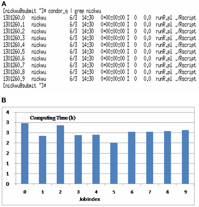
Figure 1. Running multiple chains for Bayesian LASSO in a parallel setting: (A) list of processes showing 10 running jobs; (B) computing time for the 10 jobs (numbers on the x-axis indexes jobs and the numbers on the y-axis represents computing time in hours).

From the above comparison, it is clear that parallel computing brings higher throughput, as compared with sequential computing, and total computing time for achieving the same amount of throughput is dramatically reduced.

Parallel Computing – Where We Can Get Started

Parallel Computing and Measurements of Speed-Up in Computing

Parallel computing uses multiple processing elements simultaneously to solve a problem. In general, parallel computing can be achieved at different levels: bit-level, instruction level, data parallelism, and task parallelism. The first category (bit-level) is related to the development of the computer hardware. The second category (instruction level) refers to parallelism achieved by computer programs. Data parallelism is parallelism inherent in program loops, which focuses on distribution of the data across different computer nodes to be processed in parallel. Task parallelism is the characteristic of a parallel program in that entirely different calculations can be performed on either the same or different sets of data. Task parallelism contrasts with data parallelism, where the same calculation is performed on the same or different sets of data. Thus, task parallelism does not usually scale with the size of a problem.

Computationally, many large problems can be divided into smaller jobs, which can then be solved concurrently. This is known as parallel computing, which has potential to dramatically speed-up an algorithm. Arguably, any large computational problem may consists of several parallelized parts and several non-parallelizable (sequential) parts. Then, how much can parallelization speed-up the computation? The Amdahl law states that the overall speed-up in computing available from parallelization is limited by a small portion of the program which cannon be parallelized (Amdahl, 1967), and the relationship is described by the equation:

where S is the speed-up of the program (as a factor of its original sequential runtime), and P is the fraction that is parallelizable. For example, if the sequential part of a program is 10% of the runtime, we have 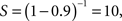indicating that we can get no more than a 10× speed-up, regardless of how many processors are added. This number puts an upper limit on the usefulness of adding more parallel execution units. In an extreme case, if a task cannot be partitioned in parallel, the application of more effort has no effect on the schedule because S = 1. Similarly, Gustafson’s (1988) law states that:

where P is the number of processors, S is the speed-up, and α is the non-parallelizable part of the process. The difference is that the speed-up (S) in the Gustafson’s law is a function of the number of processors (P), but the Amdahl’s law assumes a fixed problem size and the size of the sequential section is independent of the number of processors.

Simple Batch Processing for Parallel Computing

Batch processing is a simple way to automate the execution of a series of programs (“jobs”) on a computer without manual intervention. This is in contrast to “online” or interactive programs, which prompt the user for such input. A program takes a set of data files as input, processes the data, and produces a set of output data files. This operating environment is termed “batch processing,” because the input data are collected into batches on files and are processed in batches by the program. As an illustrative example, let modBayesB be a program implementing a BayesB analysis, in which an arbitrary portion of markers is assumed to have no effect at all, and effects of the remaining markers are associated with different variances (Meuwissen et al., 2001). This program accepts a trait name as the input argument at run time, with all other parameters provided by a parameter file. Furthermore, assume that there are k traits to be analyzed, denoted by trait_1, trait_2, …, trait_k. A sequential execution of the k jobs is to run an executable batch file containing the k jobs in any order, such as:

      modBayesB trait_1
      modBayesB trait_2
      ……
      modBayesB trait_k

In multiple-core computers, the above jobs can be run in parallel. In a Linux workstation, for example, save the follow commands into a text file, e.g., mytest.bat.

      nohup modBayesB trait_1 > out1 &
      nohup modBayesB trait_2 > out2 &
      ……
      nohup modBayesB trait_k > outn &

Then, change the property of this text file to be executable. Executing this file will lead to the n jobs running virtually in parallel in the background of the workstation. Parallel computing within a multi-core workstation is simple, but very limited in term of scalable jobs and computing throughput.

Computer Clusters and Batch Queuing Systems

Computer clusters have been increasingly used in the past two decades for high-throughput/performance computing. A cluster is a collection of interconnected parallel or distributed machines that may be viewed and used as a single, unified computing resource. Clusters can consists of homogeneous or heterogeneous collection of serial and parallel architecture computers, or even sub-clusters. For example, a cluster may consist of twenty 16-core Linux workstations, which altogether will provide 320 CPU cores for computing. The main specifications of each machine can be as follows: Dell R410 servers/workstations; 2x Intel Xeon X5660, 6-core CPUs (12 cores total); 24G Memory; 2 × 3.5′ 500 GB SATA disk; Built in IPMI. These computers will be linked to hubs which, in turn, feed into a single switch using fast Ethernet, e.g., 100 Mbit s⁻¹. Computer clusters usually improve performance and availability and are typically much more cost–effective, as compared with single computers of comparable speed or availability (Bader and Pennington, 2001).

To provide management functions and abstractions that allow clusters to work as a single resource, a number of specialized resource management software products have been developed. These include batch queuing systems for tightly interconnected clusters, such as DQS, GNQS, PBS, EASY, LSF, and LoadLeverler, and extended batch systems for loosely interconnected clusters, such as Condor, PRM, CCS, and Codine (Buyya, 1999). Simply put, such a system is a first-come first-serve queueing system, in which any user can submit a job to be run, and can kill and remove their own jobs. For example, Condor is a distributed batch system developed at the University of Wisconsin–Madison from 1988 to execute long-running jobs on available workstation and PCs, designed for HTC (Thain et al., 2005). Condor has been used to manage workload on a dedicated cluster of computers, and/or to farm out work to idle desktop computers, also called cycle scavenging. Running on multiple operation systems (OS), such as Linux, Unix, Mac OS X, FreeBSD, and contemporary Windows OS, Condor can seamlessly integrate both dedicated resources (rack-mounted clusters) and non-dedicated desktop machines (cycle scavenging) into one computing environment. For example, the NASA Advanced Supercomputing (NAS) facility Condor pool consists of approximately 350 (Silicon Graphics Inc., SGI) and Sun workstations used for software development, visualization, email, document preparation, and so on. As a scheduler software, Condor was used to distribute jobs for the first draft assembly of the Human Genome.

Parallel Computing in Condor HTC Environment

We show how Condor can be used to distribute parallel computing jobs. Assume that we have an R program that implements BayesCpi analysis in which the parameter π describes the portion of markers (genes) with no effect on the quantitative trait and the effects of the remaining markers share the same variance. The program takes parameter values from a parameter file, and it also accepts up to two parameters at run time, one for the trait name and the other for the pi (π) value, whose values overwrite those provided from the parameter file. The second parameter π is optional. When it is missing, the parameter π is treated as an unknown quantity and inferred from its posterior distribution. If a value is provided, then the pi parameter is fixed to this value in the analysis. Notice that BayesCpi analysis typically refers to the former case when π is unknown and inferred. Now, define a shell script, namely run_BayesCpi_condor, with the following content:

#use a single parameter file
statMod=“wgse_BayesCpi_beta.R”

#at least one arg is needed
if [ $# == 0 ]
then
   echo “You must specify trait name!”
   exit
fi

# specify trait name
trtNam=$1
if [ $# == 2 ]
then
   piVal=$2
fi

cd $destDir
if [ $# == 1 ]
then

   Rscript $statMod -t $trtNam
else
   Rscript $statMod -t $trtNam -n $piVal
fi

We wish to run BayesCpi analysis for the 11 traits in parallel. A Condor batch script can be defined as follows and saved as “runBayesCpi”:

Universe = vanilla
Executable = run_BayesCpi_condor
Arguments = weanin
Log = step.$(process).log
Output = step.$(process).out
Error = step.$(process).error
should_transfer_files = YES
when_to_transfer_output = ON_EXIT
transfer_input_files = parameters_Bayes.R, phenotypes_0610.csv, genotypes_0610a.csv
QueueArguments = poswea
Queue

Arguments = sc18
Queue
Arguments = musc
Queue
Arguments = docil
Queue
Arguments = rep
Queue
Arguments = rea
Queue
Arguments = bkfat
Queue
Arguments = rump
Queue
Arguments = heifer
Queue
Arguments = stay
Queue

In the above, weanin, poswea, sc18, …, stay are trait names. Furthermore, “Universe = vanilla” means a plain job (there are some special universes in Condor, such as the “standard” universe), “Executable = ” specifies the name of program to be run, “Arguments = ” provides the arguments to be used by the program, “Log = ” specifies the name of a file where Condor will record information about the job’s execution, “Output = ” specifies where Condor should put the standard output from the job, in the analysis, “Error = ” specifies where Condor should put the standard error from your job, “should_transfer_files = ” tells Condor whether or not it should transfer files, “when_to_transfer_output = ” gives technical details about when files are to be transported back to the computer from which were submitted, and “transfer_input_files = ” specifies a list of files to be transferred at run time.

Now, we submit these jobs in the Merial Condor using the condor_submit command. The status of these processes can be monitored by the condor_q command.

[wuxiaoli@condor1 ∼]$ condor_submit runBayesCpi
[wuxiaoli@condor1 ∼]$ condor_q
……(Here, information about the submitter should be displayed.)
ID OWNER SUBMITTED RUN_TIME ST PRI SIZE CMD
104.0 wuxiaoli 11/11 17:37 0+07:59:44 R 0 390.6 run_BayesCpi_condor e
104.1 wuxiaoli 11/11 17:37 0+07:59:44 R 0 390.6 run_ BayesCpi _condor e
104.2 wuxiaoli 11/11 17:37 0+07:59:44 R 0 390.6 run_ BayesCpi _condor e
104.3 wuxiaoli 11/11 17:37 0+07:59:44 R 0 390.6 run_ BayesCpi _condor e
104.4 wuxiaoli 11/11 17:37 0+07:59:44 R 0 390.6 run_ BayesCpi I_condor e
104.5 wuxiaoli 11/11 17:37 0+07:59:44 R 0 390.6 run_ BayesCpi I_condor e
104.6 wuxiaoli 11/11 17:37 0+07:59:44 R 0 390.6 run_ BayesCpi _condor e
104.7 wuxiaoli 11/11 17:37 0+07:59:44 R 0 366.2 run_ BayesCpi _condor e
104.8 wuxiaoli 11/11 17:37 0+07:59:44 R 0 390.6 run_ BayesCpi _condor e
104.9 wuxiaoli 11/11 17:37 0+07:59:44 R 0 390.6 run_ BayesCpi _condor e
104.10 wuxiaoli 11/11 17:37 0+07:59:44 R 0 390.6 run_ BayesCpi _condor e
11 jobs; 0 idle, 11 running, 0 held

High-Throughput Computing Via Pipelining for Genomic Selection

Pipelining for Increasing Computing Throughput

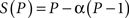
Now that we have had some experience with submitting parallel jobs in a Condor pool, it is time for us to get the flavor of pipelining for HTC. Actually, pipelining is not something new to us, but a natural concept in everyday life. For instance, consider the assembly of a car. Possible steps in the assembly line are the installation of the engine, the hood, and the wheels (in that order, with arbitrary interstitial steps). Such an automobile assembly line increases the manufacturing throughput. In computer science, pipeline refers to a set of data processing elements connected in series, so that the output of one element is the input of the next (Figure 2). The elements of a pipeline are often executed in parallel or in a time-sliced fashion. The procedure can be divided into stages, each completing a part of an instruction. The stages are connected to each other to form a pipe: instructions enter at one end, progress through the stages, and exit at the other end. Pipelining increases the CPU instruction throughput, that is, the number of instructions completed per unit of time, leading to lower total execution time and higher instruction throughput.

FIGURE 2

Figure 2. Pipelining with sequential (upper) and parallel (middle and lower) execution. Here, S1–S4 can be viewed as four stages of the computing job, and each of them can consist of sub-stages such as S2a, S2b, and S2c.

In Condor, Directed Acyclic Graphic Manager (DAGMan) is a program that allows one to specify the dependencies between your Condor jobs and automatically manages them for you. Assume that you have three jobs: job A for data input, QC, and editing, job B for feature selection (e.g., stepwise regression), and program C for post-selection inference and cross-validation. The order to execute these jobs is as follows: Do not run job B until job A has completed successfully, and do not run job C until job B has completed successfully (Figure 3).

FIGURE 3

Figure 3. A DAG with three sequential jobs.

So, a DAG is the data structure used by DAGMan to represent these dependencies: each job is a node in the DAG, and each node can have any number of “parents” or “children” nodes, as long as there are no loops.

Next, assume that we have four jobs: A for data input, QC, and data editing, B and C for feature selection each using two different criteria, and job D for comparing the two panels obtained from jobs B and C by cross-validation. A DAG can be defined, say in a file called demo.dag, which lists each of its nodes and their dependencies (Figure 4).

FIGURE 4

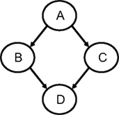
Figure 4. A DAG with four nodes (among them jobs B and C run in parallel).

Job A a.sub

Job B b.sub

Job C c.sub

Job D d.sub

Parent A Child B C

Parent B C Child D

To start the DAG job, simply run condor_submit_dag with the .dag file

      $ condor_submit_dag demo.dag

Then, condor_submit_dag submits a Scheduler Universe job with DAGMan as the executable. DAGMan acts as a scheduler, managing the submission of your jobs to Condor based on the DAG dependencies. While running a DAG, DAGMan holds and submits jobs to the Condor queue at the appropriate times, as defined in the .dag file. Once the DAG is complete, the DAGMan job itself is finished and exits. In case of a job failure, DAGMan continues until it can no longer make progress and then creates a “rescue” file with the current state of the DAG. The rescue file can be used later to restore the prior state of the DAG once the failed job is ready to be re-run. When that job completes, DAGMan will continue the DAG as if the failure never happened.

Application to Genomic Selection of Livestock

Next, we illustrate how pipelining can be used for genetic evaluation of candidate gene effects on quantitative traits. In reality, while data from candidate genes studies have been accumulated in large volumes in recent decades, it is possible to select subsets of these candidate genes that can provide alternative panels for predicting genetic merit in genomic selection. The analysis starts with data input and editing (S1). Next, panels of candidate genes that significantly affect the quantitative trait will be selected according to certain criteria (S2). Finally, predictive accuracy of these panels will be compared using cross-validation (S3). Thus, a pipeline can be formed that automate all these steps (Figure 5). Instead of DAGMan, many scripting languages can be very useful to build pipelines and/or manage pipelining jobs. In this example, these are seven R programs, three for S1 and two for S2, and for S3, respectively. Instead of using DAGMan, a Perl wrapper program can be used to manage these processes into a functional pipeline. Furthermore, multiple pipelines can be run in parallel, where each pipeline processes data for one trait based on one or more statistical methods, and as such, the computing throughput can be dramatically increased.

FIGURE 5

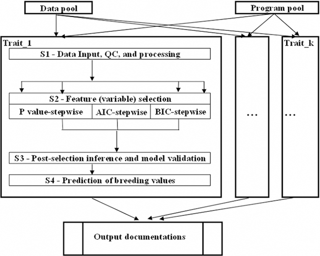
Figure 5. Workflow of a high-throughput computing pipeline for predicting genetic merit using candidate gene panels.

The example data consist of 2,246 animals, each genotyped for 384 candidate genes, with EBVs for 15 traits. A linear model was used in the data analysis, which includes EBV as the response variables and additive marker effects as the predictors. Stepwise regression analysis was used for variable (gene) selection based on P-values, Akaike’s information criterion (AIC; Akaike, 1974), and Bayesian information criterion (BIC; Schwarz, 1978), respectively.

Fifteen jobs, each corresponding to one trait, were submitted to a HTC cluster at UW (Figure 6). The analyses were implemented using the pipeline developed specifically for genomic selection (Wu et al., 2010). These jobs were queued after submission and subsequently took turns running on available machines (also called nodes). The stage for data input, QC, and processing completed quickly. At the stage of variable selection, stepwise regression based on AIC, BIC, and P-value were used for feature selection for each trait, activating a total of 45 parallel jobs. Upon completion, results were transferred back to the submit machine (Figure 7A) and deployed in web folders with secured access (Figure 7B).

FIGURE 6

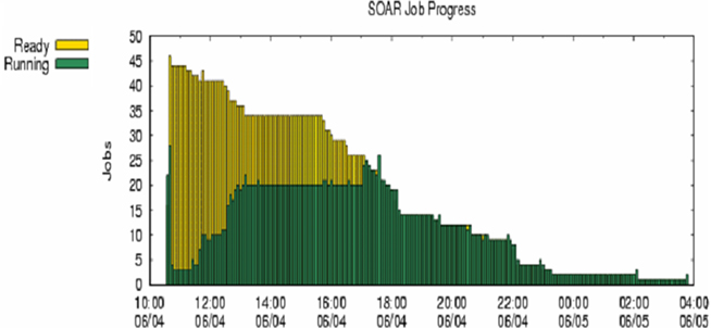
Figure 6. Running and waiting time in parallel computing for prediction of genetic merit using candidate genes for 15 quantitative traits, each with three alternative methods for feature selection. Here, x-axis represents time of computing, and y-axis represents number of jobs pending (yellow bars) and number of jobs running (green bars).

FIGURE 7

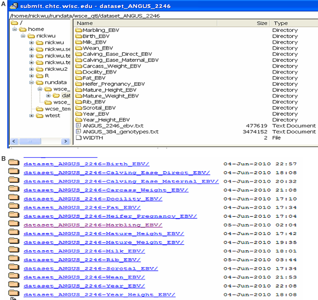
Figure 7. Results stored on the submit machine (A) and also deployed in web-accessible folders (B).

Going Further – What Opportunities Do We Have?

Though the concept of HTC may still be considered to be new to many researchers in animal breeding and genetics, the HTC revolution has already happened, as reflected in the development of computer hardware and software, as well as scalable parallel computing architectures. In this section, we briefly review existing computer architectures and infrastructures that can be leveraged for HTC, and explore new-generation hardware and software for massive parallel computing.

Leveraging HTC Architectures and Infrastructures for Genomic Selection

It is an undeniable fact that, nowadays, computer hardware is no longer made for serial computation. Nearly all new-generation computers have been equipped with multi-core central processors. Many different computer systems supporting HPC have emerged and are becoming increasingly widely used. These include massively parallel processors (MPP), symmetric multiprocessors (SMP), cache-coherent non-uniform memory access (CC-NUMA), distributed systems, and clusters (Hwang and Xu, 1998). Comparison of the architectural and functional characteristics of these systems can be found in Buyya (1999). Briefly, a MPP is a large parallel processing system with a shared-nothing architecture. It is typically composed of several hundred processing elements (nodes), connected through a high-speed interconnection network (switch). In a MPP, each node can have a variety of hardware computers, but generally consists of a main memory and one or more processors. Each node runs a separate copy of the operating system. SMP systems usually have from 2 to 64 processors, and are considered to have a shared-everything architecture. In these systems, the processors share all the global resources available, such as bus, memory, and I/O system. A single copy of the operating system runs on these systems. CC-NUMA is a scalable multiprocessor system having a CC-NUMA. This system gets its name from the non-uniform times to access the nearest and most remote parts of memory. Like an SMP, every processor in a CC-NUMA system has a global view of all of the memory. A distributed system consists of multiple independent computers that communicate through a computer network, interacting with each other in order to achieve a common goal. Each computer runs its own operating system.

On the other hand, many HTC infrastructures have already been built, though very few of them have been used for genomic selection. At the UW–Madison campus, for instance, there are existing HTC infrastructures that can be leveraged for genomic selection, in terms of CPU capacity, network connectivity, storage availability, and middleware connectivity. For CPU capacity, we can make use of the many computer clusters across the UW–Madison campus, which are linked together to share resources via technology developed by the UW Condor Team. These campus installations include the currently existing Grid Laboratory of Wisconsin (GLOW) resources, the Center for High-Throughput Computing (CHTC) resources, and the Department of Computer Sciences (DCS) cluster. Together these clusters represent over 6,200 CPU cores for computing. These machines follow a roughly 4 year replacement cycle, and as such vary between 2.0 GHz single core machines and 1 GB of RAM per CPU, to more recent multi-core machines. For network connectivity, the UW network is currently comprised of a 10 GB backbone with 10 GB connections to heavy-use buildings and departments, and 1 GB connections to the rest. The existing computational infrastructures can be used for HTC in genomic selection programs. Furthermore, the UW CHTC has off-campus collaborators. When the local UW computer resources become not sufficient, grid middleware connectivity can play an essential role. In this area, the UW is an active participant in NSF TeraGrid activities and a leading institution for the NSF/DOE Open Science Grid (OSG). These grid-based HTC resources will further enhance our computing capability and facilitate infusing HTC and grid computing techniques into genomic selection.

GPU-Enabled Massive Parallel Computing – Reinventing Wheels that Can Fly

In comparison to the traditional data processing pipeline residing on CPU, performing general-purpose computations on a graphics processing unit (GPU) is a new concept even to the computing field at large. The central processors have been evolving in both clock speeds and core counts. In the meantime, the state of graphics processors have been undergone a dramatic revolution as well. The late 1980s and early 1990s have witnessed the growth in popularity of graphically driven operating systems such as Microsoft Windows, and latter in turn helped create a market for a new type of processor. In the early 1990s, users began purchasing 2D display accelerators for their PCs. These display accelerators offered hardware-assisted bitmap operations to assist in the display and usability of graphics operating systems. From a parallel computing standpoint, NVIDIA’s release of the GeForce 3 series (chips) in 2001 possibly represented the most important breakthrough in GPU technology. Essentially, the GPUs of the early 2000 were designed to produce a color for every pixel on the screen using programmable arithmetic units known as pixel shaders. Because the arithmetic being performed on the input colors and textures was completely controlled by the programmer, it was observed that these input “colors” could actually be any data. So, if the inputs were actually numerical data signifying something other than color, then programmers could program the pixel shaders to perform arbitrary computation on this data. Because of its high arithmetic throughput, GPU-enabled computing has promised massive throughput which otherwise can not be obtained from the central processor’s traditional computing.

Toward this effort, NVIDIA’s Compute Unified Device Architecture (CUDA) makes parallel programming and using thousands of simultaneous threads straightforward. In computer science, a thread of execution is the smallest unit of processing that can be scheduled by an operating system. Simply put, CUDA is a way to write parallel C code for various CUDA-enabled graphics processors. CUDA can be downloaded from the NVIDIA web site², and it is free! A toy example of GPU parallel programming for adding two vectors is shown in Figure 8. A CUDA C program is similar to a standard C program, except a couple of noticeable differences. First, CUDA C adds the _global_ qualifier to standard C. This part alerts the compiler that a function should be compiled to run GPU (referred to as a device) instead the CPU (referred to as the host). Second, a function that executes on the device is given a different name, called a kernel. A kernel differs from a standard C function in that it contains extra parameters in the angle brackets. In this example, we have addVec <<< 1, N >>> (x, y, z), where the first number represents the number of blocks we would like the device to execute the kernel, and the second number represents the number of threads per block we would like the CUDA runtime to create on our behalf. The total number of threads running simultaneously for a given kernel is the product of those two parameters. In this example, if we define the value of the first parameter to be N = 512 and the value of the second parameter to be 1, then the total number of threads running concurrently is 512. In addition, nvcc is used to compile the CUDA part of the code, instead of gcc used by the standard C, and the debugger and profilers are therefore different.

FIGURE 8

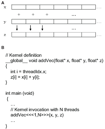
Figure 8. Illustration of GPU-enabled parallel computing: (A) graphic representation of summing two vector x and y into vector z; (B) CUDA C code (partial) for summing two vectors.

Nowadays, most computers are equipped with at least one CUDA-enabled GPU. Unfortunately, the statistical packages currently available are not designed to accommodate these new features provided by GPU-enabled massive computing. Thus, these packages will have to be re-engineered accordingly. This represents a tremendous task that may revolutionize the software development for genomic selection. An analog is like reinventing the wheels: while “traditional wheels” are designed so that they can only run on roads, the next-generation “wheels” can fly as well. In high-throughput/performance applications for genomic selection, this is saying that we will have to rebuild statistical packages for massive parallel computing on heterogeneous platforms that contains both CPU and GPU.

To summarize, the HTC revolution has already taken place, and the age of HTC for genomic selection is right here. We expect that HTC has the potential to bring revolutionary changes to genomic selection programs, such as faster solutions, better statistical methods, more informed decisions, and more competitive products. In the animal breeding industry, this new-generation computing solution represents a tremendous competitive edge in the marketplace, because it can give users the ability to quickly model their data and subsequently manipulate a product or process to see the impact of various decisions before they are made. To this end, we anticipate that HTC will have a profound impact on post-genome era selection programs in animals and plants, and it will eventually change our view and our routine practice of data analysis and decision-making involved in genomic selection.

Conflict of Interest Statement

The authors declare that the research was conducted in the absence of any commercial or financial relationships that could be construed as a potential conflict of interest.

Acknowledgments

This research was supported by the University of Wisconsin (UW) Foundation, the genomic selection grant of the Merial Ltd., and National Research Initiative competitive grant no. 2009-35205-05099 from the USDA National Institute for Food and Agriculture Animal Genome Program (Washington, DC, USA). William Taylor at the UW Center for High-Throughput Computing (CHTC) is acknowledged for technical assistance. Yao Chen is acknowledged for helping make graphs 1, 2, and 3. The BayesCpi program was modified from an example R program used in the short course taught by Dr. R. L. Fernando at the Iowa State University.

Footnotes

1. ^http://cran.r-project.org/
2. ^www.nvidia.com/cuda

References

Abdi, H. (2007). “Bonferroni and Šidák corrections for multiple comparisons,” in Encyclopedia of Measurement and Statistics, ed. N. J. Salkind (Thousand Oaks, CA: Sage), 103–107.

Akaike, H. (1974). A new look at the statistical model identification. IEEE Trans. Automat. Contr. 19, 716–723.

Amdahl, G. (1967) “The availability of the single processor approach to achieving large-scale computing capabilities,” in Proceedings of AFIPS Spring Joint Computer Conference (Atlantic City, NJ: AFIPS Press), 483–485.

Bader, D. A., and Pennington, R. (2001). Cluster computing: applications. Int. J. High Perform. Comput. Appl. 15, 181–185.

Berman, F., Fox, G. C., and Hey, A. J. G. (2003). “The grid: past, present, future,” in Grid Computing: Making the Global Infrastructure a Reality, eds F. Berman, G. C. Fox, and A. J. G. Hey (Chichester: Wiley), 9–50.

Buyya, R. (1999). High Performance Cluster Computing: Programming and Applications. Upper Saddle River, NJ: Prentice Hall PTR.

de los Campos, G., Naya, H., Gianola, D., Crossa, J., Legarra, A., Manfredi, E., Weigel, K., and Cotes, J. M. (2009). Predicting quantitative traits with regression models for dense molecular markers and pedigree. Genetics 182, 375–385.

Pubmed Abstract | Pubmed Full Text | CrossRef Full Text

Dowd, K., and Severance, C. (2010). High Performance Computing, 2nd Edn. Cambridge: O’Reilly.

Eadline, D. (2009). High Performance Computing. Hoboken, NJ: Wiley Publishing.

Gelman, A., and Rubin, D. B. (1992). Inference from iterative simulation using multiple sequences. Stat. Sci. 7, 457–511. [with discussion].

Goddard, M. E., and Hayes, B. J. (2007). Genomic selection. J. Anim. Breed. Genet. 124, 323–330.

Pubmed Abstract | Pubmed Full Text

Gustafson, J. L. (1988). Reevaluating Amdahl’s law. Commun. ACM 31, 532–533.

CrossRef Full Text

Habier, D., Fernando, R. L., and Dekkers, J. C. M. (2007). The impact of genetic relationship information on genome-assisted breeding values. Genetics 177, 2389–2397.

Pubmed Abstract | Pubmed Full Text

Habier, D., Fernando, R. L., and Dekkers, J. C. M. (2009). Genomic selection using low-density marker panels. Genetics 182, 343–353.

Pubmed Abstract | Pubmed Full Text | CrossRef Full Text

Hamblin, M. T., Buckler, E. S., and Jannink, J. L. (2011). Population genetics of genomics-based crop improvement methods. Trends Genet. PMID: 21227531. [Epub ahead of print].

Pubmed Abstract | Pubmed Full Text

Hayes, B. J., Bowman, P. J., Chamberlain, A. J., Verbyla, K. L., and Goddard, M. E. (2009). Accuracy of genomic breeding values in multi-breed dairy cattle populations. Genet. Sel. Evol. 41, 51.

Pubmed Abstract | Pubmed Full Text

Heffner, E. L., Sorrells, M. E., and Jannink, J. L. (2009). Genomic selection for crop improvement. Crop Sci. 49, 1–12.

CrossRef Full Text

Hwang, K., and Xu, Z. (1998). Scalable Parallel Computing: Technology, Architecture, Programming. New York, NY: WCB/McGraw-Hill.

Keane, T. M., Naughton, T. J., and McInerney, J. O. (2007). MultiPhyl: a high-throughput phylogenomics webserver using distributed computing. Nucleic Acids Res. 35, W33–W37.

Pubmed Abstract | Pubmed Full Text

Legarra, A., Robert-Granie, C., Manfredi, E., and Elsen, J.-M. (2008). Performance of genomic selection in mice. Genetics 180, 611–618.

Pubmed Abstract | Pubmed Full Text | CrossRef Full Text

Lorenzana, R., and Bernardo, R. (2009). Accuracy of genotypic value predictions for marker-based selection in biparental plant populations. Theor. Appl. Genet. 120, 151–161.

Pubmed Abstract | Pubmed Full Text

Maltsev, N., Glass, E., Sulakhe, D., Rodriguez, A., Syed, M. H., Bompada, T., Zhang, Y., and D’Souza, M. (2006). PUMA2-grid-based high-throughput analysis of genomes and metabolic pathways. Nucleic Acids Res. 34, D369–D372.

Pubmed Abstract | Pubmed Full Text

Meuwissen, T. H. E., Hayes, B. J., and Goddard, M. E. (2001). Prediction of total genetic value using genome-wide dense marker maps. Genetics 157, 1819–1829.

Pubmed Abstract | Pubmed Full Text

Ren, R., and Orkoulas, G. (2007). Parallel Markov chain Monte Carlo simulations. J. Chem. Phys. 126, 211102.

Pubmed Abstract | Pubmed Full Text

Schmidberger, J. W., Bate, M. A., Reboul, C. F., Androulakis, S. G., Phan, J. M., Whisstock, J. C., Goscinski, W. J., Abramson, D., and Buckle, A. M. (2010). MrGrid: a portable grid based molecular replacement pipeline. PLoS ONE 5, e10049. doi: 10.1371/journal.pone.0010049

Pubmed Abstract | Pubmed Full Text | CrossRef Full Text

Schwarz, G. (1978). Estimating the dimension of a model. Ann. Stat. 6, 461–464.

CrossRef Full Text

Sulakhe, D., Rodriguez, A., D’Souza, M., Wilde, M., Nefedova, V., Foster, I., and Maltsev, N. (2005). GNARE: automated system for high-throughput genome analysis with grid computational backend. J. Clin. Monit. Comput. 19, 361–369.

Pubmed Abstract | Pubmed Full Text

Thain, D., Tannenbaum, T., and Livny, M. (2005). Distributed computing in practice: the condor experience. Concurr. Comput. 17, 323–356.

Van Raden, P. M., Van Tassell, C. P., Wiggans, G. R., Sonstegard, T. S., Schnabel, R. D., Taylor, J. F., and Schenkel, F. S. (2009). Invited review: reliability of genomic predictions for North American Holstein bulls. J. Dairy Sci. 92, 16–24.

Pubmed Abstract | Pubmed Full Text | CrossRef Full Text

Wu, X.-L., Yao, C., Long, N., Stewart, B., Woodward, B., Mujibi, D. F. N., Rosa, G. J., Weigel, K. A., and Gianola, D. (2010). “WGSE – preliminary deployment of a high-throughput computing pipeline for genome-enabled selection,” in Plant and Animal Genome XIX Conference, San Diego.

Zhong, S., Dekkers, J. C. M., Fernando, R. L., and Jannink, J. L. (2009). Factors affecting accuracy from genomic selection in populations derived from multiple inbred lines: a barley case study. Genetics 182, 355–364.

Pubmed Abstract | Pubmed Full Text | CrossRef Full Text