Cost–Effective Prediction of Gender-Labeling Errors and Estimation of Gender-Labeling Error Rates in Candidate-Gene Association Studies

We describe a statistical approach to predict gender-labeling errors in candidate-gene association studies, when Y-chromosome markers have not been included in the genotyping set. The approach adds value to methods that consider only the heterozygosity of X-chromosome SNPs, by incorporating available information about the intensity of X-chromosome SNPs in candidate genes relative to autosomal SNPs from the same individual. To our knowledge, no published methods formalize a framework in which heterozygosity and relative intensity are simultaneously taken into account. Our method offers the advantage that, in the genotyping set, no additional space is required beyond that already assigned to X-chromosome SNPs in the candidate genes. We also show how the predictions can be used in a two-phase sampling design to estimate the gender-labeling error rates for an entire study, at a fraction of the cost of a conventional design.

Introduction

This work proposes a cost–effective approach to predict sample gender-labeling errors and estimate gender-labeling error rates in candidate gene case–control studies, when Y-chromosome data are unavailable but genotypes and intensities are available for SNPs in candidate genes. (By the “gender labeling” of a genotyped sample, we mean the self-reported gender of the study subject associated with that sample.) As long as the genotyping data set contains SNPs in candidate genes on the X-chromosome, the approach requires no extra space for additional gender-prediction SNPs.

For SNP microarray and genome-wide association data that include SNPs on the X- and Y-chromosomes, sample sexing can be determined by heterozygosity of the X-chromosome SNPs and the presence of Y-chromosome SNPs. For studies without X- or Y-chromosome SNPs, sex typing by PCR is currently the best strategy (Tzvetkov et al., 2010). Methods of sex typing are based on the human amelogenin gene, whose homologs AMELX and AMELY are located on the X- and Y-chromosomes, respectively. Current methods for sex determination for forensic and other laboratory purposes rely on genotyping small differences between the two genes (Graham, 2006), such as a 6-bp deletion in AMELX (Sullivan et al., 1993). However, this method requires that each sample be tested by PCR. Alternative high-throughput methods use single nucleotide differences between the AMELX and AMELY genes to determine sex (Tzvetkov et al., 2010). While these assays do not require special laboratory equipment, they all require labor-intensive laboratory work. In contrast, the proposed method aims to reduce the labor associated with gender checking while remaining simple and applicable to existing data from candidate-gene studies. By increasing the feasibility and cost–effectiveness of quality assurance in laboratory handling procedures, it can play a role in any integrated laboratory system for candidate-gene association studies.

If only genotypes of X-chromosome SNPs are available, gender errors (generally due to samples that have been switched with a sample of a different sex) can be predicted in male-labeled samples with excess heterozygosity or in female-labeled samples with excess homozygosity for X-chromosome SNPs. However, when there is genotyping error and a small number of X-chromosome SNPs, this heterozygosity approach can be prone to false-positive results. Our approach adds precision to heterozygosity methods by incorporating information on the intensity of X-chromosome SNPs in candidate genes relative to autosomal SNPs from the same sample. To our knowledge, no published method provides a similar framework incorporating the relative X-chromosome intensities. In essence, the X-chromosome intensities of different samples are calibrated using the autosomal intensities as a proxy for the quality and concentration of the sample. The method is described in Illumina GoldenGate genotype assay data, but may be generalized to other genotyping techniques for which intensity data are available. In addition, by validating true gender in these flagged samples and in a small proportion of samples that are not suspected to have gender-labeling errors, our approach can be used to estimate the overall gender-labeling error rates for a study. The estimation procedure saves laboratory costs by avoiding exhaustive gender checking, and yet loses little statistical precision relative to exhaustive checking when predictions correlate well with true gender. Our methods, which are intended for candidate-gene association studies rather than forensics applications, were applied successfully to a study with nine X-chromosome SNPs.

Materials and Methods

Data

Data were from a case–control genetic association study of non-Hodgkin lymphoma in which 1536 SNPs were genotyped at The Centre for Applied Genomics, Hospital for Sick Children in Toronto, using an Illumina GoldenGate genotyping platform (Illumina Inc., San Diego, CA, USA) in DNA extracted from 428 blood and 811 lymphocyte samples. The samples used in this study have been previously described (Spinelli et al., 2007). The data and quality control procedures are described in Data Sheet 1 in Supplementary Material. Illumina GenTrain scores above zero indicated reliable detection of 1444 SNPs on the autosomes and 11 SNPs on the X-chromosome. Of the 1239 blood and lymphocyte samples, 1210 passed basic quality control filters. Of the 11 X-chromosome SNPs, 9 passed basic quality control filters. In the genotyping quality control step, all intensity data were visually inspected and SNPs with clustering suggestive of copy number variations were removed. Self-reported gender information was available for all samples.

Statistical Software

All statistical analyses were performed within the R free-software environment for statistical computing (R Development Core Team, 2010). An R script and two simulated example data sets are provided in Data Sheets 2–4 in Supplementary Material to allow readers to apply the approach for predicting gender-labeling errors and estimating gender error rates.

Prediction of Gender-Labeling Errors

Our approach to identifying potential gender-labeling errors is based on two ideas. First, X-chromosome SNP genotyping intensities and heterozygosity can be used to predict the true gender of a sample. Second, a useful prediction equation for true gender can be built from the labeled gender because the majority of samples are correctly gender labeled. In essence, predicted values of gender that are discordant with labeled gender indicate potential gender-labeling errors. X-chromosome SNP genotyping intensities were normalized to the intensities of the autosomal SNP genotypes, as follows.

Method to Adjust X-Chromosome Genotype Intensity

In theory, the sample mean intensity across X-chromosome SNPs reflects a combination of the gender of the sample, the quality of the sample, and the sample concentration on the genotyping plate. Exact sample concentrations vary depending on the quantification method used and the stochastics of resampling. Therefore, variables that might reflect sample concentration were considered as potential predictors for adjusting the intensity. In our study, these variables included: (1) sample DNA concentration on the genotyping plate; (2) sample DNA concentration in the tube from which the DNA was transferred to the genotyping plate; (3) sample mean intensity across autosomal SNPs; (4) sample call rate across autosomal SNPs; (5) sample mean GenCall score (the GenCall score is an Illumina BeadArray metric for ranking and filtering out failed genotypes, DNAs, and/or loci; Oliphant et al., 2002) across autosomal SNPs; and (6) sample type (lymphocyte versus whole blood). The sample mean intensity, call rate, and GenCall score were averaged over all available autosomal SNPs. As the sample call rate across autosomal SNPs was highly correlated with the mean GenCall score across autosomal SNPs (r = 0.99), we did not consider sample call rate in further analyses. Other studies might use different predictor variables.

To check the linear relationship between the mean X-chromosome intensity and each of the six possible predictor variables for the intensity adjustment, flexible additive models were fit to the mean X-intensity using the gam function in the R package mgcv, with automatic selection of the smoothing parameter based on cross-validation. When necessary, predictor variables were transformed to reduce the influence of high-leverage points. As all relationships appeared to be linear, a multiple linear regression model was fit to all the available data, with X-intensity as the response and the six possible variables (or their transformations) considered as the predictors. After stepwise deletion at a significance threshold of p = 0.05, only the sample mean GenCall score and the sample mean intensity across autosomal SNPs remained in the final model. The sample concentration on the plate was not predictive of the sample mean intensity across X-chromosome SNPs; neither was the sample concentration in the tube, nor the sample type. This could be because the genotyping plates were constructed as uniformly as possible, with the same amount of DNA from each sample. This final model was fit to 1210 samples and 9 X-chromosome SNPs that passed quality control, and the residuals were taken as the adjusted X-intensities.

Gender-Prediction Equation

The prediction equation was obtained by fitting a generalized additive logistic model for labeled gender (Wood, 2006) with automatic selection of the smoothing parameter based on cross-validation, as implemented in the mgcv package (Wood, 2008). The additive predictors were the adjusted X-intensity and proportion of heterozygous X-chromosome SNPs. Fitting this model gives a predicted probability of being labeled male.

Y-Chromosome PCR Assays

Two sets of primers were used to amplify two different genomic regions (Battiloro et al., 1997). The first set (SRY-FWD 5^′-TATAAGTATCGACCTCGTCGGAAG-3^′ and SRY-REV 5^′-AGCCAATGTTACCCGATTGTCCTA-3^′) was used to amplify a 258-bp fragment of the SRY gene coding sequence. The second set (BLM-FWD 5^′-TGGATTCTTTGCTCAGTTGG-3^′ and BLM-REV 5^′-TTTGGGGTGGTGTAACAAA-3^′), which served as a control to determine the ability of a DNA sample to be amplified by PCR, was used to amplify a 553-bp fragment of the BLM gene coding sequence on chromosome 15. All primers were ordered at 50 nmol scale from Invitrogen by Life Technologies (Carlsbad, CA, USA). Each PCR reaction contained both sets of primers for each sample. PCR reactions were carried out in a volume of 10 μl containing 10 ng of genomic DNA, 1 mM MgSO₄, each of the four primers at 0.5 μM, 0.2 mM dNTPs, 1× Pfx Amplification Buffer and 0.25 units Platinum Pfx DNA polymerase (Invitrogen, Burlington, ON, Canada). A programmable thermal cycler (MJResearch DNA Engine 2 Tetrad) was used for the PCR reactions for a total of 30 cycles (30 s at 94°C, 90 s at 60°C and 30 s at 73°C).

PCR products were run on a 2% agarose gel (Lonza; Basel, Switzerland), stained with ethidium bromide (Sigma-Aldrich, St. Louis, MO, USA), and visualized on a gel documentation system (Fuji LAS-4000) to confirm amplification and sizes of the products. CEPH 10859 and CEPH 10853 DNA (Coriell Institute for Medical Research; Camden, NJ, USA) positive controls were used to confirm the success of the PCR experiments.

Assignment of True Gender

First we categorized the 1210 samples into 6 strata based on the labeled gender and the fitted probability of being labeled male, as summarized in Table 1. In our study, the majority of labeled males had probabilities >0.8, whereas most labeled females had probabilities <=0.2. Hence the strata with probabilities >0.8 may be viewed as “likely male,” those with probabilities <=0.2 as “likely female” and those with probabilities between 0.2 and 0.8 as “inconclusive.” Partitioning of these three probability categories according to labeled gender produces six strata that can be considered concordant (predicted and labeled gender agree for strata 1 and 6), discordant (predicted and labeled gender disagree for strata 2 and 5), or inconclusive (predicted gender is inconclusive for strata 3 and 4). As the strata are based on the distribution of the fitted probability, they might be defined differently in other studies. We applied PCR gender checking to blood and lymphocyte samples that were either discordant or inclusive (i.e., in strata 2–5), on 16 of the 18 plates in the study, or male-labeled and heterozygous at any of the 9 X-chromosome SNPs without GenCall score restrictions. To assign true gender, we used the results of PCR checking unless otherwise noted. Two of the female-labeled samples had no PCR results but had gender errors arising from known sample switches, and so were counted as errors. We were able to assign true gender to a total of 190 samples as summarized in Table 1.

TABLE 1

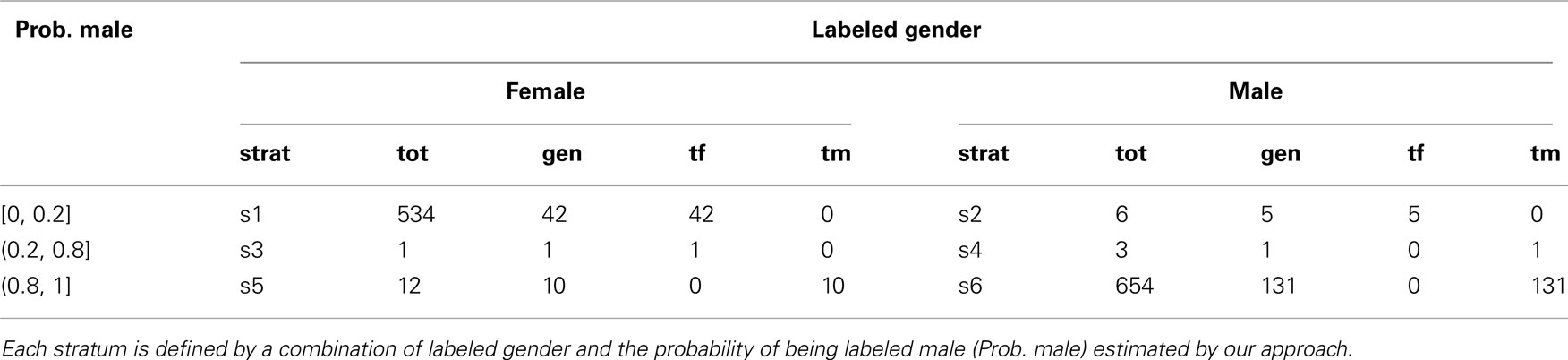
Table 1. Stratum labels (strat), numbers within each stratum (tot), numbers within strata of known true gender (gen) and true gender counts (tf = true female, tm = true male, tf + tm = gen).

Two-Phase Sampling Design to Estimate Gender-Labeling Error Rates

To estimate the accuracy of the gender prediction algorithm and the laboratory-processing gender error rates, we used a two-phase sampling design. The first phase information was comprised of labeled gender and the estimated gender-labeling probabilities, as summarized in Table 1. This information was used to direct efforts in a strategic way for the labor-intensive validation of true gender in the second phase of the sampling design. Sampling strata more likely to contain gender-labeling errors were targeted for gender validation in the second phase. To obtain an idea of the background rate of gender-labeling error, we also validated true gender in a small proportion of the samples that were predicted as unlikely to be gender-labeling errors (see Table 2). A two-phase design can give comparable precision to exhaustively determining the true gender on all samples at a fraction of the cost (e.g., Breslow and Chatterjee, 1999). The efficiency of a sampling design is defined as its ability to yield precise estimators of parameters (Cain and Breslow, 1988). Stratified sampling is efficient when variation of the second-phase variable within strata is small compared to variation between strata (Lohr, 1999, section 4.5). Provided true gender is well correlated with labeled gender and estimated gender-labeling probability, little variation of true gender within strata is expected. In this case, efficiency gains are realized by judicious choice of sampling fractions rather than by extensive gender determination (e.g., Reilly and Pepe, 1995). Two principles guided our choice of sampling fractions. First, sampling fractions should be larger in strata with larger variation in true gender as in, for example, Neyman allocation (Neyman, 1938; Lohr, 1999, p. 108). As variation in true gender is expected to be highest in the discordant or inconclusive strata, we aimed for 100% sampling there (Table 1). Second, for a fixed sample-size at the second phase, the balanced design with roughly equal numbers per stratum is easily implemented and has good efficiency (e.g., Breslow and Chatterjee, 1999). Hence, we also aimed to follow up a slightly larger number of samples for true gender in the concordant strata than the maximum that were followed up in the discordant or inconclusive strata. As the maximum number of samples per stratum in the discordant or inconclusive strata was 12 (see Table 1), we decided to confirm true gender for 15 samples each in the concordant strata, for sampling fractions of 2.8 and 2.3%, respectively (see Table 2). From the 190 eligible samples whose true gender could be assigned, we randomly selected 15 samples each from the concordant strata. In the discordant or inconclusive strata, we were able to assign gender to all but one sample in stratum 2, two samples in stratum 4, and two samples in stratum 5. As summarized in Table 2, this sampling strategy led to a total of 47 samples in the second phase. The true gender assignment for the 47 second-phase samples is summarized in Table 2. To verify that within-strata variation in true gender is small relative to between-strata variation, we estimated the proportion of total variation in the true gender captured by the strata. A proportion near unity suggests little is to be gained from sampling more than 15 samples in the concordant strata. We emphasize that the second-phase sample of 47 is intended to illustrate the potential savings in laboratory effort arising from a two-phase sampling design. The extra information about the true gender of the 190 samples was used to validate the results of the two-phase sampling approach.

TABLE 2

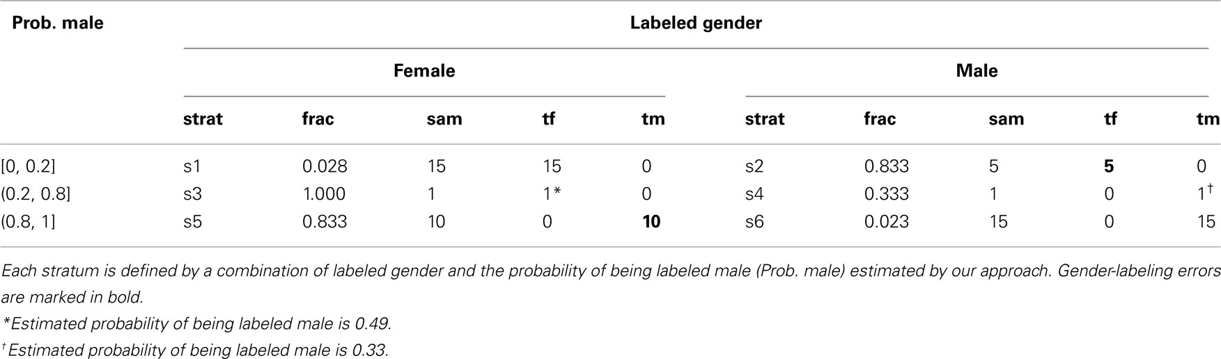
Table 2. Stratum labels (strat), second-phase sampling fractions (frac), numbers in second-phase sample (sam = frac × tot, where tot is given in Table 1), and true gender counts (tf = true female, tm = true male, tf + tm = sam).

Accuracy of Gender Prediction

The accuracy of the prediction algorithm depends on how well it separates the samples according to their true gender. Traditionally, accuracy is measured by the AUC, defined by the area under the receiver operating characteristic (ROC) curve, with an AUC of 1 representing perfect prediction and an AUC of 0.5 representing random predictions. We used inverse-probability weighting (e.g., Lumley, 2004) to estimate the ROC curve based on stratified samples of true gender for 47 and 190 samples.

Calculation of the Gender Error Rates

Let Z be the true gender with males coded as Z = 1 and females coded as Z = 0. Let Y be the labeled gender with labeled males coded as Y = 1 and labeled females coded as Y = 0. We used the function svyglm in the survey package of R (Lumley, 2010) to fit a logistic regression model of the probability of being labeled male given true gender: logit(P(Y = 1|Z)) = β₀ + β₁ Z. The package uses inverse-probability weighting to adjust for the biased sampling. Within each of the six strata, we assume that any of the samples that are missing true gender status (due to failed PCR) are missing completely at random. Under the logistic model,

is the gender-labeling error rate in females and

is the gender-labeling error rate in males.

We used these gender-labeling error rates and Bayes rule to estimate how well the gender labeling predicts the actual gender of a sample as follows. Let X be the three-category version of the fitted probabilities of being male (i.e., probabilities <=0.2, 0.2–0.8, and >0.8). Let S = S(X, Y) be the stratum variable for the second-phase sampling of the true gender Z, with S = i, for i = 1, 2, …, 6. We estimated P(Z|Y) using the equation P(Z|Y) = P(Y|Z)*P(Z)/P(Y), where P(Z) was calculated as P(Z|S = 1)P(S = 1) + P(Z|S = 2)P(S = 2) + … + P(Z|S = 6) P(S = 6); and P(Y|Z) is the gender-labeling error rate calculated above. The stratum-specific conditional probabilities P(Z|S = i) were estimated from the 47 samples in the second phase of the study which had information on true gender. The stratum-specific probabilities P(S) and the gender label probabilities P(Y) were estimated from all 1210 samples in the study.

Summary of Statistical Methods and Their Goals

In summary, we apply a multiple linear regression model to adjust X-chromosome intensity for sample characteristics such as autosomal intensity, quality of the sample and sample concentrations. We then use these adjusted X-chromosome intensities along with the proportions of heterozygous X-chromosome SNPs as predictors in a generalized additive logistic model of labeled gender. The resulting gender predictions along with the labeled gender define the sampling strata for a two-phase sampling design. After balanced sampling of true gender from the strata, we apply inverse-probability weighting to estimate the accuracy of the gender prediction algorithm and the gender-labeling error rates for the entire study. By applying Bayes rule, the gender-labeling error rates can be used to estimate how well the gender-labeling predicts the true gender of a sample.

Other Gender Prediction Methods

We compared our approach for predicting gender-labeling errors, with an arbitrary probability threshold of 0.5, to the approaches implemented in PLINK (Purcell et al., 2007), Golden Helix ( Bozeman, MT, USA, www.goldenhelix) and PLATO (Grady et al., 2010). Briefly, the heterozygosity-based approach in PLINK uses X-chromosome genotypes to calculate a moment estimator of the inbreeding coefficient F and makes a male call if F > 0.8 and a female call if F < 0.2. We took PLINK predicted gender errors to be samples whose call disagrees with their gender labeling. The heterozygosity-based approach in Golden Helix uses non-missing X-chromosome SNPs to predict gender errors in female samples with heterozygosity values <0.1 and in male-labeled samples with heterozygosity values >0.1. In the absence of Y-chromosome markers, the intensity-based approach in Golden Helix uses the average of log intensity ratios (logR) for a sample across X-chromosome SNPs. The measurement logR is commonly used to determine copy number status and can be calculated by log₂(observed intensity/reference intensity), where reference intensity is calculated using a reference panel of mixed gender to determine the normal baseline intensity expected at each marker. For example, because females have two copies of the X-chromosome, their mean logR values should be greater than zero whereas males, with only one copy, should have mean logR values less than zero. Thus, Golden Helix flags female-labeled samples with mean logR less than zero and male-labeled samples with mean logR greater than zero. PLATO flags male-labeled samples with heterozygosity values greater than a user-specified upper threshold or less than a user-specified lower threshold. We took PLATO predicted gender errors to be male-labeled samples with positive heterozygosity (i.e., upper threshold 0).

Results

Prediction of Gender-Labeling Errors

We started by considering the normalized genotyping intensity (R value) available in the raw data of the Illumina GoldenGate genotype data set. For a given sample, we focused only on successfully called X-chromosome SNPs and defined the mean X-intensity and proportion of heterozygous X-chromosome SNPs to be, respectively, the sample’s average genotype intensity and the proportion of heterozygous calls in these SNPs. As males are hemizygous at X-chromosome SNPs, they are not expected to be called as heterozygotes, and the intensities (R values) of their X-chromosome SNPs should be about half of those of females. These observations motivate a simple plot of the sample mean X-intensity versus proportion of heterozygous X-chromosome SNPs for all the samples. Ideally, one should see two separate clusters for males and females. However, this simple plot ignores the noise in the intensity measurements that is introduced by the quality of the sample and its concentration on the genotyping plate. Better clustering of male and female samples was obtained by statistically adjusting the sample mean X-intensity for variables related to the quality and concentration of the sample.

The adjusted sample mean X-intensity plotted against the proportion of heterozygous X-chromosome SNPs is shown in Figure 1. In the figure, data forms into vertical bars because, with nine X-chromosome SNPs, a given sample may be heterozygous at zero, one, two, and theoretically up to nine SNPs. We see only eight main vertical bars because, for the majority of samples with genotypes for all nine SNPs, none were heterozygous at eight or more. Intermediate heterozygosities result from samples with genotypes available for fewer than nine SNPs. From this plot, it is evident that a small number of labeled males have heterozygous calls. Such calls could be the result of genotyping error or sample switches involving different genders. For the most part, however, the female- and male-labeled samples are clearly separated. We therefore used the adjusted mean X-intensity and the proportion of heterozygous X-chromosome SNPs as predictor variables in subsequent model fitting. The fitted model gives a predicted probability of being labeled male. In our study, the majority of labeled males had probabilities >0.8, whereas most labeled females had probabilities <=0.2.

FIGURE 1

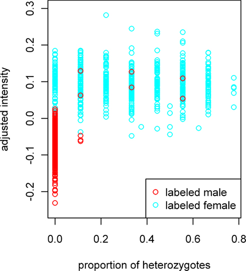
Figure 1. Adjusted X-chromosome intensity versus proportion of heterozygous X-chromosome SNPs. Data forms into vertical bars because, with nine X-chromosome SNPs, a given sample may be heterozygous at zero, one, two, and theoretically up to nine SNPs. We see only eight main vertical bars because no samples with genotypes for all nine SNPs were heterozygous for eight or more SNPs. Intermediate heterozygosities result from samples with genotypes for fewer than nine SNPs. X-chromosome intensity values on the vertical axis have been adjusted for the sample mean GenCall score and sample mean intensity across autosomal SNPs, as described in the text.

Validating Predicted Gender-Labeling Errors

PCR assays were used to check the samples flagged with potential gender-labeling errors. Samples flagged included those with intermediate fitted probabilities of being labeled male (0.2–0.8), female-labeled samples with high fitted probabilities of being labeled male (0.8–1), and male-labeled samples with low fitted probabilities of being labeled male (0–0.2). Results for samples flagged for potential gender-labeling errors are given in Tables 3 and 4 for male-labeled and female-labeled samples, respectively. Table 3 includes male-labeled samples not flagged by our approach that would have been flagged by heterozygosity-based approaches because they are heterozygous at least one X-chromosome SNP. However, to conserve space and effort, Table 4 excludes the 64 female-labeled samples not flagged by our approach that would have been flagged by heterozygosity-based approaches because they are homozygous at all nine X-chromosome SNPs. Based on estimated haplotype frequencies, we expect about 60 female samples to have X-chromosome heterozygosity values of zero.

TABLE 3

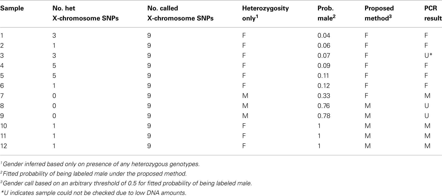
Table 3. Summary of results for male-labeled samples flagged by our approach or by positive heterozygosity values.

TABLE 4

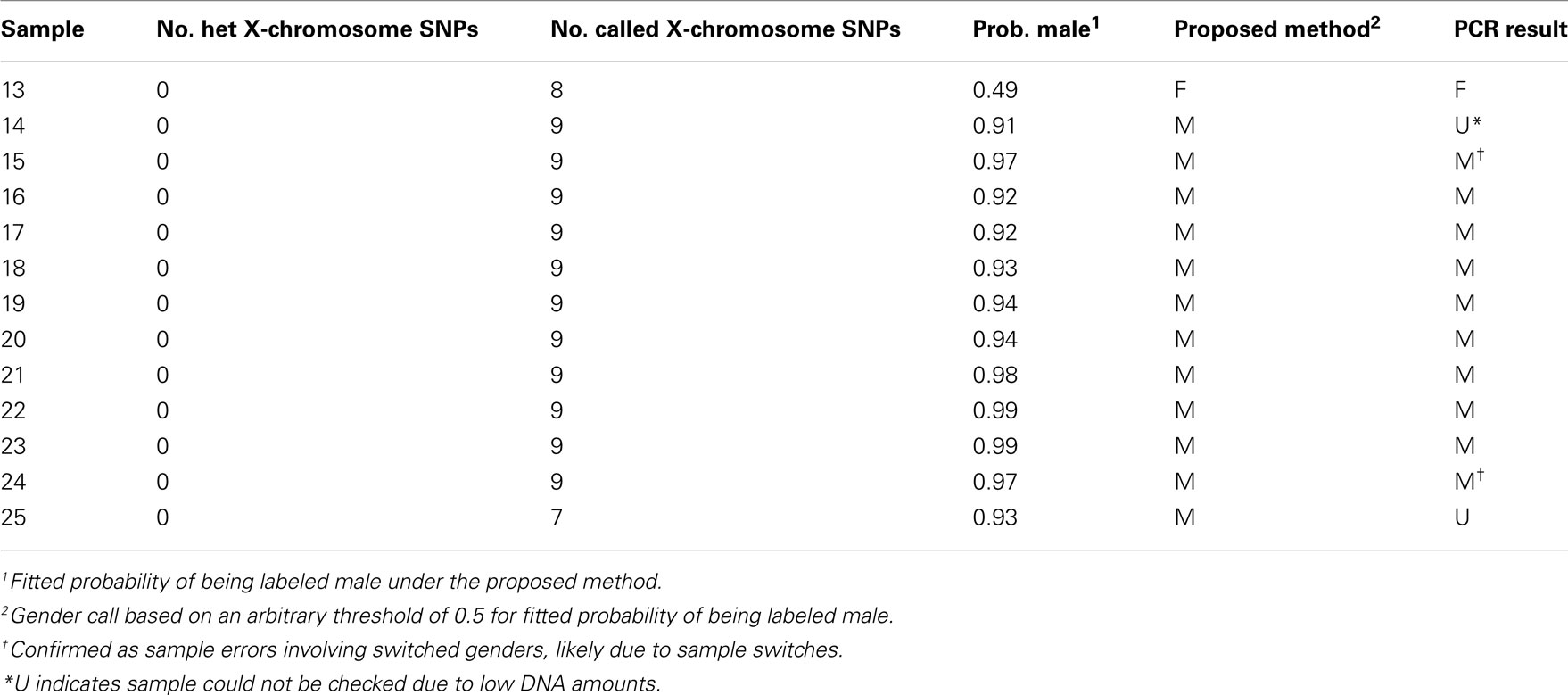
Table 4. Summary of results for female-labeled samples flagged by our approach.

In general, the approach marks female-labeled samples with low intensities and homozygosity and predicts them to be male, whereas male-labeled samples with either heterozygous calls or high intensities are predicted to be female. Figure 2 shows the plot of adjusted mean X-intensity versus proportion of heterozygous X-chromosome SNPs for labeled males and labeled females, respectively, with different symbols used for predicted gender errors in labeled males and labeled females.

FIGURE 2

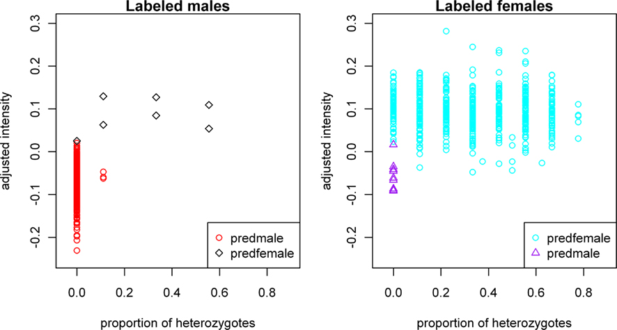
Figure 2. Plot of gender-labeling errors predicted by our approach. Subjects in the left panel are labeled male samples; “predfemale”: predicted probability of being male less than 0.5. Subjects in the right panel are labeled female samples; “predmale”: predicted probability of being male greater than or equal to 0.5. X-chromosome intensity values on the vertical axes have been adjusted for the sample mean GenCall score and sample mean intensity across autosomal SNPs, as described in the text.

Based on an arbitrary threshold of 0.5 for the fitted probability of being labeled male, we predicted seven gender errors in male-labeled samples, ascertained true gender for six of these seven predicted gender errors and confirmed five of them as true females. In the male-labeled samples, the error discovery rate, defined as the number of confirmed gender errors in the flagged samples divided by the number of flagged samples whose true gender was ascertained, is thus 5/6 = 83.3%. The standard approach to predicting male-labeled gender errors on the basis of one or more heterozygous genotypes at X-chromosome SNPs has an error discovery rate of 5/8 = 62.5%. We also predicted 12 gender errors in female-labeled samples based on the same gender-calling threshold of 0.5. We were able to ascertain true gender for 10 of these 12 predicted gender errors and all 10 were confirmed as males. Eight of these 10 confirmed male samples were identified through Y-chromosome PCR assays and two were known switches with samples of a different gender during processing or extraction. In female-labeled samples, the error discovery rate was thus 100%.

The estimated AUC of the gender prediction procedure, based on second-phase samples of true gender for either 47 or 190 samples, was essentially unity, representing essentially ideal predictions.

Estimating Gender Error Rates

In what follows, all probabilities are with respect to the population of 1210 genomic DNA samples from whole blood or lymphocytes with DNA on the genotyping plates. We emphasize that the 47 samples taken in the second phase are not random samples from this reference population. Rather, we have used biased sampling with preference going to certain strata defined on the basis of labeled gender and the predicted probability of being male, as indicated in Table 2.

Based on the true gender observed for the 47 biased samples in the second phase, we estimated the conditional probabilities of incorrect gender labeling to be P(labeled male|true female) = 0.011 (approximate 95% CI 0.005–0.025) and P(labeled female|true male) = 0.018 (95% CI 0.010–0.032). Note that gender-labeling error rates will tend to be lower than the laboratory error rates, as mislabeling of same-sex samples will go undetected. We also estimated the predictive probabilities of gender labeling to be P(true female|labeled female) = 0.998 and P(true male|labeled male) = 0.991.

Efficiency of the Sampling Design

To compare the efficiency of the two-phase design relative to a naive design that verified the true gender for all the samples, we estimated the proportion of total variation in the true gender captured by the sampling strata. As shown in Table 2, within each sampling stratum, there was no variation in the true gender. Hence all variation in the observed values of true gender can be explained by the sampling strata, and the two-phase design should be efficient. To verify this, we applied the same approach to all 190 samples with true gender assigned (Table 1), and obtained the same point and interval estimates of the error rates and the same true gender prediction probabilities as with the 47 second-phase samples. These results suggest that the design is highly efficient and that there is little to be gained by testing additional samples by PCR.

Comparison to Other Gender Prediction Methods

There were 77 female-labeled samples that were homozygous at all non-missing X-chromosome SNPs. All 77 of these female-labeled samples were flagged by PLINK and the Golden Helix heterozygosity-based approach. PLATO does not consider female-labeled samples when checking for potential gender errors. There were nine male-labeled samples that were heterozygous at any X-chromosome SNP. All nine of these male-labeled samples were flagged by the Golden Helix heterozygosity-based approach and by PLATO. There were 15 confirmed gender errors, 10 in labeled females and 5 in labeled males. In the female-labeled samples, our approach, PLINK, and the Golden Helix heterozygosity-based approach identified 10/10 and the Golden Helix intensity-based approach identified 8/10 of the confirmed errors. In male-labeled samples, our approach, PLATO and the Golden Helix heterozygosity-based approach identified 5/5; the Golden Helix intensity-based approach identified 4/5 and PLINK identified 3/5 of the confirmed errors. Thus, our approach and the Golden Helix heterozygosity-based approach were able to identify all confirmed errors. As summarized in Table 5, our approach flagged far fewer female-labeled samples than the other approaches and, as a consequence, its error discovery rate was higher in labeled females. All approaches flagged a comparable number of male-labeled samples, except for the Golden Helix intensity-based approach which flagged far more. Of the methods considered, overall, our approach had the lowest number of false-positive results.

TABLE 5

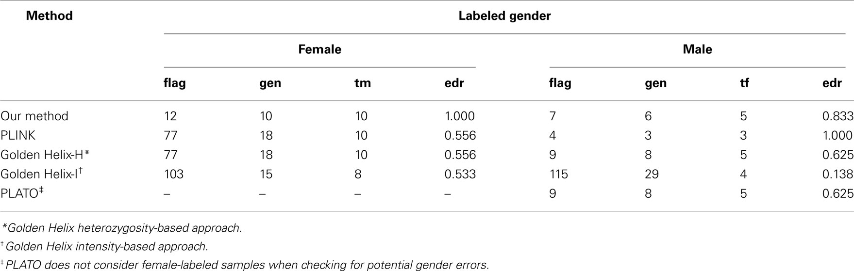
Table 5. Method-specific numbers of flagged samples (flag) with true gender ascertained (gen), numbers of confirmed gender errors (tf = true female, tm = true male) among these, and error discovery rate (edr).

Discussion

We have described a statistical approach to predict gender-labeling errors and estimate gender-labeling error rates in candidate-gene association studies when Y-chromosome data are unavailable, but some X-chromosome SNPs are in the genotyping set. In the prediction step of our approach, we identify potential gender-labeling errors by using the genotypes of the X-chromosome SNPs and their intensities, normalized to the intensities of the autosomal SNP genotypes of the same sample. In the subsequent estimation step, we use the samples identified as potential gender-labeling errors, along with a small proportion of the samples not suspected to have gender-labeling errors, to estimate the gender-labeling error rates for the entire study. The strategic sampling in the second step enables efficient estimation of the gender-labeling error rates without having to validate the true gender for all study samples. Taken together, these two steps provide a useful tool for laboratory-processing quality assurance.

By incorporating information about the intensity of X-chromosome SNPs, the approach adds value to standard methods of error prediction based solely on heterozygosity. To our knowledge, no published methods formalize a framework in which to use the X-chromosome intensity values adjusted for autosomal intensity, as well as heterozygosity. The proposed approach works well in both male- and female-labeled samples from our candidate-gene association study. The results helped reveal a small number of sample processing issues.

We explored alternate models for predicting gender-labeling errors. For instance, we tried using both the GenTrain score (a genotype clustering score for Illumina GoldenGate genotyping data) and the proportion of called X-chromosome SNPs to construct two sets of weights defining the proportion of heterozygous X-chromosome SNPs. We also tried a third predictive model based on the number rather than the proportion of heterozygous X-chromosome SNPs. All three of these alternate models led to the same results as the proposed approach. Finally, we tried fitting a model using binary indicators of heterozygous calls for each of the nine X-chromosome SNPs; the use of this model did not improve predictions relative to the proposed approach. Though each of these alternate models for predicting gender-labeling errors gave similar results with our data on nine SNPs, there may have been differences between the approaches had more X-chromosome SNPs been included.

We have also shown how the predictions for gender mislabeling can be used to estimate the gender-labeling error rates for the entire study in a cost–effective manner. Relative to exhaustive validation of gender, the proposed estimation approach costs considerably less and yet loses little precision, provided that predictions correlate well with true gender in both male- and female-labeled samples (e.g., Reilly and Pepe, 1995). Efficiency is achieved by strategic follow up of problematic samples identified in the prediction step. By checking only 4% of the samples, we were able to estimate the gender-labeling error rates for the whole study, enabling substantial savings in time and laboratory work.

With nine X-chromosome SNPs, we observed improved precision to predict gender errors from incorporating intensity information relative to approaches based on heterozygosity alone. In light of this, it is natural to ask the general question of how many markers are needed before heterozygosity-based methods catch up in precision. The answer depends on factors such as the variability of intensities at each X-chromosome SNP, the genotyping error rates at each X-chromosome SNP, their minor allele frequencies (MAFs) and their dependence structure in the population. We therefore consider the related but simpler question of how many SNPs would be required to clearly separate the 547 female samples and 663 male samples based on heterozygosity alone. For this optimal number of SNPs, incorporating additional intensity information will be pointless. To address this simpler question, we predict a gender error whenever a sample’s heterozygosity is more likely under the opposite gender. To render calculations tractable, we assume X-chromosome SNPs with independent genotypes, common MAF p and common genotyping error rate ε = 1/1000. Assuming independent and identically distributed genotyping errors at each SNP, such that heterozygotes are equally likely to be miscalled as either homozygote but homozygotes are miscalled only as heterozygotes, the number of heterozygous genotypes in either gender is a binomial random variable with number of trials equal to the number of X-chromosome SNPs and success probability equal to ε in males and 2p(1 − p) + ε(1 − 2p)² in females. We define female and male samples to be clearly separated if the expected numbers of false predictions in 547 females and in 663 males are both no more than one. As possible values for p, we consider the minimum (0.060), median (0.257), and maximum (0.418) MAF of X-chromosome SNPs in our study. In this idealized scenario, 88, 19, and 14 SNPs, respectively, are required to achieve separation. However, it should be noted that these calculations ignore the dependence between SNPs in our data, which would increase the number of SNPs required.

The methods we propose are intended for research studies with a reasonable quality of DNA sources, genotyped under general laboratory conditions. The methods would not be suitable for forensic applications involving DNA sources of very limited quantity and quality. When applied to data from candidate-gene association studies, our methods offer several advantages, including ease of implementation and speed. Gender-labeling errors can be predicted with existing custom-designed genotyping sets, provided that X-chromosome SNPs are in the candidate genes. In our study, we were able to accurately predict several sample switches with data from only nine X-chromosome SNPs in two candidate genes. This accuracy was achieved in spite of dependence in the six X-chromosome SNPs of one of the candidate genes (with 0.46≤|r|≤0.80 for most SNPs). For the prediction step, no additional laboratory experiments are required. Crucially, our approach can correct for the variable performance of different sample types, in this case whether DNA was extracted from blood or from lymphocytes. It allows sample processing issues to quickly come to the surface and, if necessary, be addressed by changes in protocol, and allows erroneous samples from gender switches to be identified and excluded from experiments. Additionally, our approach can be used across genotyping batches, throughout the process of sample collection and DNA extraction, permitting such issues to be identified in time for changes to be implemented or subjects to be re-sampled. Unlike other methods, this approach does not depend on the use of a single set of primers for PCR, and is thus unaffected by rare mutations in primer binding sites. Should a variant exist on the custom genotyping probe binding site, the genotyping call rate for that probe would drop if the variant is common enough, and the SNP would thus be excluded from the analysis in the quality control steps. Furthermore, our method relies on metrics collected across all probes on the X-chromosome and is thus unlikely to be affected by a single rare mutation. In theory, the approach to identifying potential gender errors could be extended to detect X-chromosome trisomies (XXY and XXX), although it would not work on sex-reversal syndromes (XY females or XX males). In this investigation, however, we have not pursued the issue of X-chromosome trisomies.

One limitation of our approach to predicting gender-labeling errors relates to copy number variants (CNVs) and large-scale duplications and deletions, which are proving to be more common than previously believed (Iafrate et al., 2004). Next-generation sequencing efforts recently demonstrated duplicated or deleted genomic regions in some human populations relative to others (Li et al., 2010). When there are only a few candidate genes on the X-chromosome, our method and any other that relies on heterozygosity or intensity can be vulnerable to bias from duplications and deletion events on the X-chromosome. Thus, our method would not be appropriate for DNA from cell lines, which are known to be particularly susceptible to such alterations. That being said, quality control protocols that remove SNPs with genotype clustering suggestive of CNVs can help mitigate the effects of such events. However, the possibility that X-chromosome SNPs could lie in deletions or duplications should be kept in mind when applying this or related approaches to predict gender mislabeling, particularly when few X-chromosome SNPs are used. To assess potential bias arising from inter-population variation in duplicated or deleted regions of the X-chromosome, we tested whether the gender-mislabeling predictions were associated with self-reported ethnicity of samples; our results were negative (p = 0.72 based on an exact test of independence).

In conclusion, we present an approach that predicts gender-mislabeling arising in plating or sample processing, whether at the collection stage, DNA extraction stage, or storage. We also show how the predictions can be used to estimate the laboratory rates of gender mislabeling in a cost–effective way. Our methods require only a small number of X-chromosome SNPs (we used only nine), which could be part of a candidate gene on the X-chromosome. However, as the number of included SNPs on the X-chromosome decreases, the prediction approach potentially becomes more vulnerable to bias from duplication and deletion events on the X-chromosome.

Conflict of Interest Statement

The authors declare that the research was conducted in the absence of any commercial or financial relationships that could be construed as a potential conflict of interest.

Acknowledgments

Thanks to Carolyn Brown for helpful discussions about molecular sexing of samples, and to Brad McNeney for helpful discussions about two-phase sampling designs. The non-Hodgkin lymphoma study (John J. Spinelli, Angela Brooks-Wilson) was supported by grants from the Canadian Cancer Society and the Canadian Institutes for Health Research (CIHR). Conghui Qu and Jeong Eun Min were supported by the Mathematics of Information Technology and Complex Systems (MITACS), Canadian Networks of Centres of Excellence and by the Natural Sciences and Engineering Council of Canada; Johanna M. Schuetz was funded by scholarships from the Alberta Heritage Foundation for Medical Research and CIHR. Jinko Graham, Denise Daley and Angela Brooks-Wilson hold Scholar or Senior Scholar Awards from the Michael Smith Foundation for Health Research. Denise Daley is a Canada Research Chair.

Supplementary Material

The Supplementary Material for this article can be found online at http://www.frontiersin.org/statistical_genetics_and_methodology/10.3389/fgene.2011.00031/abstract

Data Sheet 1. A brief description of the quality control steps applied to our data.

Data Sheet 2. This R script is provided to apply the approach in the manuscript for predicting gender-labeling errors and estimating gender error rates.

Data Sheet 3. This simulated data file can be used with the R script in Data Sheet 2. Readers can apply the script to the data in this file to see how we identified potential gender-labeling errors. The file contains information on the ID, labeled gender, average adjusted X-chromosome intensity, and proportion of heterozygous X-chromosome SNPs for 1210 simulated samples.

Data Sheet 4. This simulated data file can be used with the R script in Data Sheet 2. Readers can apply the script to the data in this file to see how we estimated gender-labeling error rates for the study. The file contains information on the ID and true gender assignments for 54 simulated samples.

References

Battiloro, E., Angeletti, B., Tozzi, M. C., Bruni, L., Tondini, S., Vignetti, P., Verna, R., and D’Ambrosio, E. (1997). A novel double nucleotide substitution in the HMG box of the SRY gene associated with Swyer syndrome. Hum. Genet. 100, 585–587.

Pubmed Abstract | Pubmed Full Text

Breslow, N. E., and Chatterjee, N. (1999). Design and analysis of two-phase studies with binary outcome applied to Wilms tumour prognosis. Appl. Stat. 48, 457–468.

Cain, K. C., and Breslow, N. E. (1988). Logistic regression analysis and efficient design of two-stage studies. Am. J. Epidemiol. 128, 1198–1206.

Pubmed Abstract | Pubmed Full Text

Grady, B. J., Torstenson, E., Dudek, S. M., Giles, J., Sexton, D., and Ritchie, M. D. (2010). Finding unique filter sets in PLATO: a precursor to efficient interaction analysis in GWAS data. Pac. Symp. Biocomput. 15, 315–326.

Graham, E. (2006). DNA reviews: sex determination. Forensic Sci. Med. Pathol. 2, 283–286.

Iafrate, A. J., Feuk, L., Rivera, M. N., Listewnik, M. L., Donahoe, P. K., Ying, Q., Scherer, S. W., and Lee, C. (2004). Detection of large-scale variation in the human genome. Nat. Genet. 36, 949–951.

Pubmed Abstract | Pubmed Full Text

Li, R., Li, Y., Zheng, H., Luo, R., Zhu, H., Li, Q., Qian, W., Ren, Y., Tian, G., Li, J., Zhou, G., Zhu, X., Wu, H., Qin, J., Jin, X., Li, D., Cao, H., Hu, X., Blanche, H., Cann, H., Zhang, X., Li, S., Bolund, L., Kristiansen, K., Yang, H., Wang, J., and Wan, J. (2010). Building the sequence map of the human pan-genome. Nat. Biotechnol. 28, 57–63.

Pubmed Abstract | Pubmed Full Text | CrossRef Full Text

Lohr, S. L. (1999). Sampling: Design and Analysis. Pacific Grove: Brooks/Cole.

Lumley, T. (2004). Analysis of complex survey samples. J. Stat. Softw. 9, 1–19.

Lumley, T. (2010). Survey: analysis of complex survey samples. R Package version 3.22-1.

Neyman, J. (1938). Contribution to the theory of sampling human populations. J. Am. Stat. Assoc. 33, 101–116.

CrossRef Full Text

Oliphant, A., Barker, D. L., Stuelpnagel, J. R., and Chee, M. S. (2002). BeadArray technology: enabling an accurate, cost-effective approach to high-throughput genotyping. BioTechniques 32, S56–S61.

Purcell, S., Neale, B., Todd-Brown, K., Thomas, L., Ferreira, M. A. R., Bender, D., Maller, J., Sklar, P., de Bakker, P. I. W., Daly, M. J., and Sham, P. C. (2007). PLINK: a toolset for whole-genome association and population-based linkage analysis. Am. J. Hum. Genet. 81, 559–575.

Pubmed Abstract | Pubmed Full Text

R Development Core Team (2010). R: A Language and Environment for Statistical Computing. Vienna: R Foundation for Statistical Computing.

Reilly, M., and Pepe, M. S. (1995). A mean score method for missing and auxiliary covariate data in regression models. Biometrika 82, 299–314.

CrossRef Full Text

Spinelli, J. J., Ng, C. H., Weber, J.-P., Connors, J. M., Gascoyne, R. D., Lai, A. S., Brooks-Wilson, A. R., Le, N. D., Berry, B. R., and Gallagher, R. P. (2007). Organochlorines and risk of non-Hodgkin lymphoma. Int. J. Cancer 121, 2767–2775.

Pubmed Abstract | Pubmed Full Text

Sullivan, K. M., Mannucci, A., Kimpton, C. P., and Gill, P. (1993). A rapid and quantitative DNA sex test: fluorescence-based PCR analysis of X-Y homologous gene amelogenin. BioTechniques 15, 636–638, 640–641.

Pubmed Abstract | Pubmed Full Text

Tzvetkov, M. V., Meineke, I., Sehrt, D., Vormfelde, S. V., and Brockmöller, J. (2010). Amelogenin-based sex identification as a strategy to control the identity of DNA samples in genetic association studies. Pharmacogenomics 11, 449–457.

Pubmed Abstract | Pubmed Full Text | CrossRef Full Text

Wood, S. (2006). Generalized Additive Models: An Introduction with R. Boca Raton: Chapman & Hall/CRC.

Wood, S. (2008). Fast stable direct fitting and smoothness selection for generalized additive models. J. R. Stat. Soc.Ser. B Stat. Methodol. 70, 495–518.