Monocular concurrent recovery of structure and motion scene flow

1. Introduction

Scene flow is the field over the image domain of the visible environmental surfaces three-dimensional (3D) velocities. Only the visible surfaces are relevant in the definition because they alone, not the occluded, contribute to visual information. As a result, the scene flow domain is the image domain: at each image point, scene flow consists of the velocity vector of the corresponding visible environmental surface point. It is the time derivative of the point 3D position.

For a working definition of scene flow, let Ω be the common domain of an image sequence I(x, t), where x = (x, y) designates image position, and t is time. For each point, x ∈ Ω, let $P^{\prime }=\frac{dP}{\mathit{dt}}$ be the velocity vector of the visible environmental point P = (X, Y, Z) projected on x. Scene flow is the velocity vector field, $F=\left(U,V,W\right)=\left(\frac{\mathit{dX}}{\mathit{dt}},\frac{\mathit{dY}}{\mathit{dt}},\frac{\mathit{dZ}}{\mathit{dt}}\right)$ over Ω. It is a function of image position and time: F = F(x, t).

Scene flow is a fundamental dimension of three-dimensional scene analysis for the obvious reason that it describes the motion of real objects in the environment. Moreover, it is related to optical flow via depth (Mitiche and Aggarwal, 2013). It can be regarded as a three-dimensional analog of optical flow: at each point x ∈ Ω, and each instant of time, scene flow is the velocity vector of the visible environmental point P, which projects on x, whereas optical flow is the velocity vector of the image of P at x.

From a broad perspective, scene flow can be computed in one of two ways: parametric and non-parametric. Parametric methods use a parametric form of the scene flow coordinates and non-parametric methods compute scene flow directly as a vector field without resorting to an intermediate representation.

Investigations of parametric scene flow generally assume that environmental objects are rigid and, therefore, decompose scene flow in terms of 3D translational and rotational parameters (Mitiche and Aggarwal, 2013). This representation leads to the Longuet–Higgins and Pradzny fundamental equations (Longuet-Higgins and Prazdny, 1980) relating the rigid motion parameters, depth, and optical flow. Depth and the rigid screw motion parameters become the unknown 3D variables to determine, from which scene flow can be recovered a posteriori. In most studies, the Longuet–Higgins and Pradzny equations underlie the recovery of rigid body structure and motion from image sequences, even when not used explicitly.

Current parametric methods can be separated into two broad categories, those which treat the case of a viewing system moving in a static environment and those which allow the viewing system and the environmental objects to move simultaneously and independently. In the first case, the problem is significantly simpler because the single 3D motion to take into account is that of the viewing system (Bruss and Horn, 1983; Adiv, 1985; Horn and Weldon, 1988; Shahraray and Brown, 1988; Heeger and Jepson, 1992; Taalebinezhaad, 1992; De Micheli and Giachero, 1994; Gupta and Kanal, 1995; Xiong and Shafer, 1995; Hung and Ho, 1999; Brodsky et al., 2000; Srinivasan, 2000; Liu et al., 2002). Moreover, segmentation of the environment into differently moving objects is not an issue in a static environment, simplifying the problem further.

The simultaneous motion of the viewing system and viewed objects has also been the subject of several studies (MacLean et al., 1994; Weber and Malik, 1997; Fejes and Davis, 1998; Mitiche and Hadjres, 2003; Mitiche and Sekkati, 2006; Sekkati and Mitiche, 2006a,b, 2007). The non-variational methods in MacLean et al. (1994), Weber and Malik (1997), and Fejes and Davis (1998) assume that optical flow is given beforehand and segment the visual field into differently moving rigid objects by grouping processes, such as region growing by 3D motion (Weber and Malik, 1997), clustering of 3D motion via mixture models (MacLean et al., 1994), and clustering via oriented projections of optical flow (Fejes and Davis, 1998).

The variational methods in Mitiche and Hadjres (2003), Mitiche and Sekkati (2006), and Sekkati and Mitiche (2006a,b, 2007) use functionals with a data term based on the Longuet–Higgins and Prazdny rigid motion model and a regularization term to account for 3D interpretation discontinuities; they mainly differ in the way these discontinuities are represented.

Non-parametric scene flow computation methods seek to recover scene flow at each point of the image domain without recourse to a parametric form of the movements or surfaces in space. Such methods are most relevant when practicable models of scene flow cannot be assumed, as with, for instance, articulated human and animal motion.

Because scene flow is related to depth, via optical flow, which they jointly define (Mitiche and Aggarwal, 2013), non-parametric scene flow computation has been generally studied in the context of stereoscopy (Zhang and Kambhamettu, 2000; Pons et al., 2003; Vedula et al., 2005; Huguet and Devernay, 2007; Wedel et al., 2008, 2011; Rabe et al., 2010; Basha et al., 2013; Vogel et al., 2013), although it stands independent of stereoscopy. Here following, we will show that non-parametric scene flow can actually be recovered from a single image sequence. We will describe a variational scheme reminiscent of the Horn and Schunck optical flow estimation method. The functional of this formulation has two terms: a data term, which relates 3D velocity to depth via the image sequence spatiotemporal variations, and a classic smoothness regularization term. The data term falls out simply by rewriting the Horn and Schunck optical flow constraint linearly in terms of scene flow and depth. The Euler–Lagrange equations corresponding to the minimization of the objective functional yield, when discretized, a large sparse system of linear equations, which can be solved efficiently by Jacobi/Gauss–Seidel iterations. The scheme can be generalized to boundary preserving formulations as in optical flow estimation (Deriche et al., 1995; Aubert et al., 1999).

The remainder of this paper is organized as follows: Section 2 formulates the problem and develops the objective functional. Section 3 deals with the optimization of the objective functional. It derives the Euler–Lagrange equations and the corresponding discrete system of linear equations in the variables of scene flow and relative depth. It also shows that the matrix of this system is symmetric positive definite, which prescribes a solution by Jacobi/Gauss–Seidel iterations. Section 4 addresses the problem of regularized spatiotemporal derivative computation and Section 5 gives experimental results.

2. Formulation

The problem is to recover scene flow and depth from an image sequence I: (x, y, t) → I(x, y, t), where (x, y) are the coordinates over the bounded image domain Ω, and $t\in {\mathbb{R}}^{+}$ is time. The formulation starts with the Horn and Schunck optical flow gradient constraint (Horn and Schunck, 1981), which relates the coordinate functions, u and v, of optical flow to the image sequence spatiotemporal variations:

$I_{x}u+I_{y}v+I_t=0,$ (1)

where I_x, I_y, I_t are the image spatiotemporal partial derivatives. Let P be a point in space (X, Y, Z), its 3D coordinates, and (x, y) its image coordinates. The viewing system model geometry is shown in Figure 1. Derivation with respect to time of the projection equations $x=f\frac{X}{Z}$ and $y=f\frac{Y}{Z}$, where f is the focal length, gives the coordinates u, v of optical velocity as functions of scene flow and depth:

$u=\frac{\mathit{dx}}{\mathit{dt}}=\frac{\mathit{fU}-\mathit{xW}}{Z};v=\frac{\mathit{dy}}{\mathit{dt}}=\frac{\mathit{fV}-\mathit{yW}}{Z},$ (2)

where Z designates depth (Figure 1) and $\left(U,V,W\right)=\left(\frac{\mathit{dX}}{\mathit{dt}},\frac{\mathit{dY}}{\mathit{dt}},\frac{\mathit{dZ}}{\mathit{dt}}\right)$ is the scene flow at P. Substitution of these optical flow expressions in the gradient constraint (1), followed by the multiplication of the left hand side by Z ≠ 0 gives the following linear constraint relating scene flow and depth to the image spatiotemporal derivatives:

$f{I}_{x}U+f{I}_{y}V-\left(x{I}_x+y{I}_y\right)W+I_{t}Z=0.$ (3)

There are two important observations to make about this linear equation. First, an obvious observation is that this equation evaluates at each point of the image domain: fI_x(x)U(x) + fI_y(x) V (x) − (xI_x(x) + yI_y(x))W (x) + I_t (x)Z (x) = 0 and, therefore, contains four unknown variables at each point. As with optical flow computation (Hildreth, 1984), this says that any local interpretation of the variables is ambiguous. Dense interpretation, i.e., global over the image domain, which is of interest to us here, will require additional constraints. In a classic way, we will use a variational statement of the problem where these additional constraints characterize the variables as smooth over the image domain.

FIGURE 1

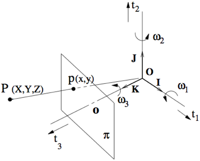
Figure 1. The viewing system is symbolized by a Cartesian reference system (O; X,Y,Z) and central projection through the origin. The Z-axis is the depth axis. The image plane π is orthogonal to the Z-axis at distance f, the focal length, from O.

The second observation is that the equation, being homogeneous, has a trivial solution, U = V = W = 0; Z = 0, in which, of course, we are not interested, and can easily avoid in practice. More importantly, since we are dealing with an actual physical problem, the environmental depth field and scene flow, which gave rise to the image spatiotemporal variations, constitute a solution but so does any scaled version of it: if (U, V, W), Z is a solution, so is k(U, V, W), kZ for some arbitrary real k. This is a limitation inherent to the recovery of 3D structure and motion from 2D image sequences (Ullman, 1983).

Theoretically, the scale can be fixed by setting the depth of a particular point, in which case the depth of any other point is relative to it. However, this is hardly an answer, because setting the depth of a point would affect a single equation out of thousands that generally make up the discrete system of equations in practice. Along a different vein, a particular solution can be picked by imposing it a given norm. For instance, we could, say, compute a unit norm solution: ||(U, V, W, Z)|| = 1 by solving under this constraint the system of equations of the problem. We will follow instead an effective simple scheme: we will adopt a variational formulation of the problem where the scale of interpretation is fixed by solving for depth Z_r relative to a fronto-parallel plane ${\mathrm{\Pi }}_{Z_0}:Z=Z_0$, for some arbitrary positive depth, Z₀. More precisely, this is done by first rewriting Eq. (3) as follows:

$f{I}_{x}U+f{I}_{y}V-\left(x{I}_x+y{I}_y\right)W+I_t\left(Z-Z_0\right)+I_t{Z}_0=0,$ (4)

and then making a change of variable Z_r ← Z − Z₀, which would give:

$f{I}_{x}U+f{I}_{y}V-\left(x{I}_x+y{I}_y\right)W+I_t{Z}_r+I_t{Z}_0=0$ (5)

For notational simplicity and economy, we can reuse the symbol Z to designate relative depth Z_r, in which case we write Eq. (5) as:

$f{I}_{x}U+f{I}_{y}V-\left(x{I}_x+y{I}_y\right)W+I_{t}Z+I_t{Z}_0=0$ (6)

By rewriting this data equation with respect to reference, plane ${\mathrm{\Pi }}_{Z_0}$ effectively fixes the scale of 3D interpretation because for another reference plane, say Z₁ = kZ₀, the equation integrity is maintained by the correspondingly scaled interpretation k(U, V, W), kZ and, inversely, for a scaled solution k(U, V, W), kZ the equation integrity is maintained by a reference plane at kZ₀. The trivial solution, which is now (0, 0, 0, −Z₀), rather than (0, 0, 0, 0), can be avoided in practice simply by initializing away from it in the iterative algorithm that we are about to develop. This iterative algorithm, as will be detailed subsequently, consists of Gauss–Seidel iterations, which at each step solve by singular value decomposition local 4 × 4 systems of linear equations resulting from the objective functional Euler–Lagrange equations.

We can now formulate the problem of joint computation of scene flow and relative depth from a single image sequence as the minimization of the following functional:

$\begin{array}{l}\mathbf{E}(U,V,W,Z|I)=\frac{1}{2}{{\displaystyle {\int }_{\Omega }(f{I}_{x}U+f{I}_{y}V-(x{I}_x+y{I}_y)W+I_{t}Z+I_t{Z}_0)}}^{2}dxdy\\ +\frac{\alpha }{2}{\displaystyle {\int }_{\Omega }(||\nabla U|{|}^2+\left|\right|\nabla V|{|}^2+||\nabla W|{|}^2)}dxdy+\frac{\beta }{2}{\displaystyle {\int }_{\Omega }\left|\right|\nabla Z|{|}^{2}dxdy,}\end{array}$ (7)

where α and β are positive constants balancing the contributions of the smoothness terms. This functional can be modified to preserve the boundaries of scene flow/depth via discontinuity preserving regularization (Deriche et al., 1995).

3. Optimization

The Euler–Lagrange equations corresponding to the objective functional (7) are the following coupled partial differential equations:

$\begin{array}{llll}\hfill & f{I}_x\left(f{I}_{x}U+f{I}_{y}V+\left(-x{I}_x-y{I}_y\right)W+I_{t}Z+I_t{Z}_0\right)-\mathrm{\alpha }{\nabla }^{2}U=0& \hfill & \\ \hfill & f{I}_y\left(f{I}_{x}U+f{I}_{y}V+\left(-x{I}_x-y{I}_y\right)W+I_{t}Z+I_t{Z}_0\right)-\mathrm{\alpha }{\nabla }^{2}V=0& \hfill & \\ \hfill & \left(-x{I}_x-y{I}_y\right)\left(f{I}_{x}U+f{I}_{y}V+\left(-x{I}_x-y{I}_y\right)W+I_{t}Z+I_t{Z}_0\right)-\mathrm{\alpha }{\nabla }^{2}W=0& \hfill & \\ \hfill & I_t\left(f{I}_{x}U+f{I}_{y}V+\left(-x{I}_x-y{I}_y\right)W+I_{t}Z+I_t{Z}_0\right)-\mathrm{\beta }{\nabla }^{2}Z=0,\end{array}$ (8)

to which we add the Neumann boundary conditions on the solution at the boundary ∂Ω of Ω:

$\frac{\mathit{\partial U}}{\partial n}=0,\frac{\mathit{\partial V}}{\partial n}=0,\frac{\mathit{\partial W}}{\partial n}=0,\frac{\mathit{\partial Z}}{\partial n}=0,$ (9)

where $\frac{\partial }{\partial n}$ is the differentiation operator in the direction of the normal n of ∂Ω.

Let Ω be discretized as a unit-spacing grid D and the grid points indexed by the integers {1,2, …, N}. Pixels are indexed in the lexicographical order, i.e., top-down and left-to-right. N = n² when the image is n × n. Let a = fI_x, b = fI_y, c = −(xI_x + yI_y), d = I_t. For all grid point I ∈ {1, 2, …, N}, a discrete approximation of the Euler–Lagrange equations (8) is:

$\begin{array}{llll}\hfill & a_i^2{U}_i+a_i{b}_i{V}_i+a_i{c}_i{W}_i+a_i{d}_i{Z}_i+a_i{d}_i{Z}_0-\mathrm{\alpha }{\displaystyle \sum _{j\in {\mathbf{N}}_i}}\left(U_j-U_i\right)=0& \hfill & \\ \hfill & b_i{a}_i{U}_i+b_i^2{V}_i+b_i{c}_i{W}_i+b_i{d}_i{Z}_i+b_i{d}_i{Z}_0-\mathrm{\alpha }{\displaystyle \sum _{j\in {\mathbf{N}}_i}}\left(V_j-V_i\right)=0& \hfill & \\ \hfill & c_i{a}_i{U}_i+c_i{b}_i{V}_i+c_i^2{W}_i+c_i{d}_i{Z}_i+c_i{d}_i{Z}_0-\mathrm{\alpha }{\displaystyle \sum _{j\in {\mathbf{N}}_i}}\left(W_j-W_i\right)=0& \hfill & \\ \hfill & d_i{a}_i{U}_i+d_i{b}_i{V}_i+d_i{c}_i{W}_i+d_i^2{Z}_i+d_i^2{Z}_0-\mathrm{\beta }{\displaystyle \sum _{j\in {\mathbf{N}}_i}}\left(Z_j-Z_i\right)=0\end{array}$ (10)

where (U_i, V_i, W_i, Z_i) = (U, V, W, Z)_i is the scene flow at i; a_i, b_i, c_i, d_i are the values at i of a, b, c, d, respectively, and N_i is the set of indices of the neighbors of i. For the four-neighborhood, card (N_i) = 4 for points interior in D, and card (N_i) < 4 for boundary points. The Laplacian ▽² Q, Q ∈ {U, V, W, Z}, in the Euler–Lagrange equations, has been discretized as $\frac{1}{4}{\sum }_{j\in N_i}\left(Q_j-Q_i\right)$, where the factor $\frac{1}{4}$ is absorbed by α and β. Rewriting (10), and where n_i = card(N_i), we have the following system of linear equations, I ∈ {1, …, N}:

$\left(S\right)\left\{\begin{array}{c}\hfill \left(a_i^2+\mathrm{\alpha }{n}_i\right)U_i+a_i{b}_i{V}_i+a_i{c}_i{W}_i+a_i{d}_i{Z}_i-\mathrm{\alpha }{\displaystyle \sum _{j\in {\mathbf{N}}_i}}{U}_j=-a_i{d}_i{Z}_0\hfill \\ \hfill b_i{a}_i{U}_i+\left(b_i^2+\mathrm{\alpha }{n}_i\right)V_i+b_i{c}_i{W}_i+b_i{d}_i{Z}_i-\mathrm{\alpha }{\displaystyle \sum _{j\in {\mathbf{N}}_i}}{V}_j=-b_i{d}_i{Z}_0\hfill \\ \hfill c_i{a}_i{U}_i+c_i{b}_i{V}_i+\left(c_i^2+\mathrm{\alpha }{n}_i\right)W_i+c_i{d}_i{Z}_i-\mathrm{\alpha }{\displaystyle \sum _{j\in {\mathbf{N}}_i}}{W}_j=-s{c}_i{d}_i{Z}_0\hfill \\ \hfill d_i{a}_i{U}_i+d_i{b}_i{V}_i+d_i{c}_i{W}_i+\left(d_i^2+\mathrm{\beta }{n}_i\right)Z_i-\mathrm{\beta }{\displaystyle \sum _{j\in {\mathbf{N}}_i}}{Z}_j=-d_i^2{Z}_0\hfill \end{array}\right.$

Let q = (q₁, …, q_4N) ^t ∈ ${\mathrm{ℝ}}^{4N}$ be the vector with coordinates q_4i–3 = U_i, q_4i–2 = V_i, q_4i–1 = W_i,q_4i = Z_i, I ∈ {1, …, N}, and r = (r₁,…r_4N)^t ∈ R^4N, the vector with coordinates r_4i–3 = −a_i d_iZ₀, r_4i–2 = −b_i d_iZ₀, r_{4 i–1} = −c_i d_iZ₀, and $r_{4i}=-d_i^2{Z}_0$, i ∈ {1, …, N}. System (S) of linear equations can be written in matrix form as:

$\mathrm{Aq}=r$ (11)

where A is the 4N × 4N matrix with elements $A_{4i-3,4i-3}=a_i^2+\mathrm{\alpha }{n}_i;A_{4i-2,4i-2}=b_i^2+\mathrm{\alpha }{n}_i$; ${\mathbf{\text{A}}}_{4i-1,4i-1}=c_i^2+\mathrm{\alpha }{n}_i;A_{4i,4i}=d_i^2+\mathrm{\beta }{n}_i$; A_{4i–3,4i–2} = A_{4i–2,4i–3} = a_ib_i; A_{4i–3,4i–1} = A_{4i–1,4i–3} = a_ic_i; A_4i–3,4i = A_4i,_4i–3 = a_id_i; A_{4i–2,4i–1} = A_{4i– 1},_4i–2 = b_ic_i; A_4i–2,4i = A_4i,_4i–2 = b_id_i; A_4i–1,4i = A_4i,_4i–1 = c_id_i; for all I ∈ {1, …, N}; A_{4i–3,4j–3} = A_4i–2,_4j–2 = A_{4i–1,4j–1} = −α and A_4i–4j = −β, for all i, j ∈ {1, …, N} such that j ∈ N_i, all other elements being equal to zero.

System (S) is a large scale sparse system of linear equations. Such systems are best solved by iterative methods designed for sparse matrices (Ciarlet, 1982; Stoer and Bulirsch, 2002). Here following, we prove that matrix A is symmetric positive definite, which implies an effective solution of Eq. (11) by 4 × 4 block-wise Gauss–Seidel iterations.

One can easily verify that matrix A is symmetric. Matrix A is also positive definite. To show this, we verify that q^tAq > 0 for all q ∈ R^4N, q ≠ 0. We have:

$\begin{array}{ll}\hfill q^t\mathrm{Aq}& ={\displaystyle \sum _{i=1}^N}\left(\left(a_i^2+\mathrm{\alpha }{n}_i\right)U_i+a_i{b}_i{V}_i+a_i{c}_i{W}_i+a_i{d}_i{Z}_i-\mathrm{\alpha }{\displaystyle \sum _{j\in {\mathbf{N}}_i}}{U}_j\right)U_i\\ \hfill & +{\displaystyle \sum _{i=1}^N}\left(b_i{a}_i{U}_i+\left(b_i^2+\mathrm{\alpha }{n}_i\right)V_i+b_i{c}_i{W}_i+b_i{d}_i{Z}_i-\mathrm{\alpha }{\displaystyle \sum _{j\in {\mathbf{N}}_i}}{V}_j\right)V_i& \hfill & \\ \hfill & +{\displaystyle \sum _{i=1}^N}\left(c_i{a}_i{U}_i+c_i{b}_i{V}_i+\left(c_i^2+\mathrm{\alpha }{n}_i\right)W_i+c_i{d}_i{Z}_i-\mathrm{\alpha }{\displaystyle \sum _{j\in {\mathbf{N}}_i}}{W}_j\right)W_i& \hfill & \\ \hfill & +{\displaystyle \sum _{i=1}^N}\left(d_i{a}_i{U}_i+d_i{b}_i{V}_i+d_i{c}_i{W}_i+\left(d_i^2+\mathrm{\beta }{n}_i\right)Z_i-\mathrm{\beta }{\displaystyle \sum _{j\in {\mathbf{N}}_i}}{Z}_j\right)Z_i\end{array}$ (12)

Following algebraic manipulations, we get:

$\begin{array}{llll}\hfill q^t\mathrm{Aq}& ={\displaystyle \sum _{i=1}^N}{\left(a_i{U}_i+b_i{V}_i+c_i{W}_i+d_i{Z}_i\right)}^2+\mathrm{\alpha }{\displaystyle \sum _{i=1}^N}\left(n_i\left(U_i^2+V_i^2+W_i^2\right)\right)+\mathrm{\beta }{\displaystyle \sum _{i=1}^N}\left(n_i\left(Z_i^2\right)\right)& \hfill & \\ \hfill & -\mathrm{\alpha }{\displaystyle \sum _{i=1}^N}\left({\displaystyle \sum _{j\in {\mathbf{N}}_i}}{U}_j{U}_i+{\displaystyle \sum _{j\in {\mathbf{N}}_i}}{V}_j{V}_i+{\displaystyle \sum _{j\in {\mathbf{N}}_i}}{W}_j{W}_i\right)-\mathrm{\beta }{\displaystyle \sum _{i=1}^N}\left({\displaystyle \sum _{j\in {\mathbf{N}}_i}}{Z}_j{Z}_i\right)\end{array}$ (13)

If we distribute the n_i terms U_i of the second row into the corresponding neighborhood sum of the third row, we will get:

$\begin{array}{llll}\hfill & {\displaystyle \sum _{i=1}^N}{n}_i{U}_i^2-{\displaystyle \sum _{i=1}^N}{\displaystyle \sum _{j\in {\mathbf{N}}_i}}{U}_j{U}_i={\displaystyle \sum _{i=1}^N}{\displaystyle \sum _{j\in {\mathbf{\text{N}}}_i;j>i}}\left(U_i^2+U_j^2-2U_j{U}_i\right)={\displaystyle \sum _{i=1}^N}{\displaystyle \sum _{j\in {\mathbf{\text{N}}}_i;j>i}}{\left(U_i-U_j\right)}^2& \hfill & \end{array}$

Using similar manipulations for the other variables (V,W,Z), we arrive at the expression we need:

$\begin{array}{llll}\hfill q^t\mathrm{Aq}& ={\displaystyle \sum _{i=1}^N}{\left(a_i{U}_i+b_i{V}_i+c_i{W}_i+d_i{Z}_i\right)}^2& \hfill & \\ \hfill & +\mathrm{\alpha }{\displaystyle \sum _{i=1}^N}{\displaystyle \sum _{j\in {\mathbf{\text{N}}}_i;j>i}}\left({\left(U_i-U_j\right)}^2+{\left(V_i-V_j\right)}^2+{\left(W_i-W_j\right)}^2\right)& \hfill & \\ \hfill & +\mathrm{\beta }{\displaystyle \sum _{i=1}^N}{\displaystyle \sum _{j\in {\mathbf{\text{N}}}_i;j>i}}\left({\left(Z_i-Z_j\right)}^2\right)\end{array}$ (14)

For q ≠ 0, we have q^t Aq = 0 if and only if the terms in both sums on the right-hand side of (14) are zero. The second-sum terms are zero if and only if the scene consists of a fronto-parallel plane (plane Z = Z₀) under constant translation ((U_i, V_i, W_i) = T). The first-sum terms are zero if and only if all vectors (a_i,b_i,c_i,d_i)_i = (I_xi,I_yi, −x_iI_xi − y_iI_yi, I_ti) lie in a hyperplane for all (x_i,y_i) ∈ D. This is possible if and only if the spatiotemporal visual pattern is null, which is an irrelevant case. Therefore, q^t Aq > 0 for q ≠ 0 and A is positive definite. This means that the point-wise and block-wise Gauss–Seidel and relaxation iterative methods for solving system (11) converge (Ciarlet, 1982; Stoer and Bulirsch, 2002).

For a 4 × 4 block division of matrix A, the Gauss–Seidel iterations consist of solving, for each i, ∈{1, …, N}, the following 4 × 4 linear system of equations, where k is the iteration number:

$\begin{array}{cc}\hfill \hfill & \hfill \left(a_i^2+\mathrm{\alpha }{n}_i\right)U_i^{k+1}+a_i{b}_i{V}_i^{k+1}+a_i{c}_i{W}_i^{k+1}+a_i{d}_i{Z}_i^{k+1}=-a_i{d}_i{Z}_0+\mathrm{\alpha }\left({\displaystyle \sum _{j\in {\mathbf{\text{N}}}_i;j<i}}{U}_j^{k+1}+{\displaystyle \sum _{j\in {\mathbf{\text{N}}}_i;j>i}}{U}_j^k\right)\hfill \\ \hfill \hfill \\ \hfill \hfill & \hfill b_i{a}_i{U}_i^{k+1}+\left(b_i^2+\mathrm{\alpha }{n}_i\right)V_i^{k+1}+b_i{c}_i{W}_i^{k+1}+b_i{d}_i{Z}_i^{k+1}=-b_i{d}_i{Z}_0+\mathrm{\alpha }\left({\displaystyle \sum _{j\in {\mathbf{\text{N}}}_i;j<i}}{V}_j^{k+1}+{\displaystyle \sum _{j\in {\mathbf{\text{N}}}_i;j>i}}{V}_j^k\right)\hfill \\ \hfill \hfill \\ \hfill \hfill & \hfill c_i{a}_i{U}_i^{k+1}+c_i{b}_i{V}_i^{k+1}+\left(c_i^2+\mathrm{\alpha }{n}_i\right)W_i^{k+1}+c_i{d}_i{Z}_i^{k+1}=-c_i{d}_i{Z}_0+\mathrm{\alpha }\left({\displaystyle \sum _{j\in {\mathbf{\text{N}}}_i;j<i}}{W}_j^{k+1}+{\displaystyle \sum _{j\in {\mathbf{\text{N}}}_i;j>i}}{W}_j^k\right)\hfill \\ \hfill \hfill \\ \hfill \hfill & \hfill d_i{a}_i{U}_i^{k+1}+d_i{b}_i{V}_i^{k+1}+d_i{c}_i{W}_i^{k+1}+\left(d_i^2+\mathrm{\beta }{n}_i\right)Z_i^{k+1}=-d_i^2{Z}_0+\mathrm{\beta }\left({\displaystyle \sum _{j\in {\mathbf{\text{N}}}_i;j<i}}{Z}_j^{k+1}+{\displaystyle \sum _{j\in {\mathbf{\text{N}}}_i;j>i}}{Z}_j^k\right),\hfill \\ \hfill \hfill \end{array}$

which can be done efficiently by the singular value decomposition method (Forsythe et al., 1977).

4. Estimation of the Spatiotemporal Derivatives

The purpose is to estimate the spatiotemporal derivatives I_x,I_y,I_t, from two consecutive images of a sequence. The estimation of a function derivative from inaccurate data is an ill-posed problem because small changes in the function values can result in arbitrarily large errors in the derivative estimated by finite differences (Terzopoulos, 1986). Therefore, image noise can adversely affect the quality of motion interpretation that uses finite difference image derivatives. In motion analysis, the problem has been generally approached by local averaging of the finite difference derivatives (Horn and Schunck, 1981). However, regularized differentiation can be more effective as we show in the following.

4.1. Differentiation by Averaging Finite Differences

Following the formulas in the Horn and Schunck paper on optical estimation (Horn and Schunck, 1981), motion analysis studies have generally used forward first differences to represent derivatives, locally averaged to counter the effect of noise:

$\begin{array}{l}{I}_x(r,c)\approx \frac{1}{4}{\displaystyle \sum _{\mathrm{\Delta }r=0}^1\left\{I(r+\mathrm{\Delta }r,c+1,0)-I(r+\mathrm{\Delta }r,c,0)+I(r+\mathrm{\Delta }r,c+1,1)-I(r+\mathrm{\Delta }r,c,1)\right\}}\\ I_y(r,c)\approx \frac{1}{4}{\displaystyle \sum _{\mathrm{\Delta }c=0}^1\left\{I(r+1,c+\mathrm{\Delta }c,0)-I(r,c+\mathrm{\Delta }c,0)+I(r+1,c+\mathrm{\Delta }c,1)-I(r,c+\mathrm{\Delta }c,1)\right\}}\\ I_t(r,c)\approx \frac{1}{4}{\displaystyle \sum _{\mathrm{\Delta }r=0}^1{\displaystyle \sum _{\mathrm{\Delta }c=0}^1\left\{I(r+\mathrm{\Delta }r,c+\mathrm{\Delta }c,1)-I(r+\mathrm{\Delta }r,c+\mathrm{\Delta }c,0)\right\}}}\end{array}$ (15)

where I₀ is the current image and I₁ the next. The spatial derivatives have sometimes been estimated using averages of central differences.

Global averaging of the finite difference approximations can be done using L² smoothing of the derivatives finite differences: a derivative estimate g is computed by minimizing:

$E\left(g\right)=\frac{1}{2}{\int }_{\mathrm{\Omega }}\left({\left(g-g_0\right)}^2+\mathrm{\gamma }\parallel \nabla g{\parallel }^2\right)\mathit{dxdy},$ (16)

where g is a partial derivative function and g₀ its finite difference approximation from I. The corresponding Euler–Lagrange equation g − g₀ − γ▽² g = 0 is then discretized to yield a large sparse system of linear of equations.

4.2. Regularized Differentiation

Although image data smoothing is commonly done in motion analysis, it does not generally solve the derivative estimation ill-posedness, so that prior de-noising of the image independently of differentiation followed by finite difference approximation is not generally effective (Chartrand, 2005). A more productive method is to state differentiation within Tikhonov regularization theory for ill-posed problems (Cullum, 1971; Hanke and Scherzer, 2001). In Hanke and Scherzer (2001), the problem was to find a smooth approximation of the true derivative y’ of a function y from given data ${\tilde{y}}_i$. This was done by determining an approximation f of y, which minimizes an objective functional having a term of discrepancy between f and the given data, and a regularization term to penalize the L² norm of f″. The derivative was subsequently evaluated on f. The objective functional in Hanke and Scherzer (2001) was investigated in earlier studies (Schoenberg, 1964; Reinsch, 1967), which showed that it is minimized by a natural cubic spline. In Cullum (1971), the differentiation process itself was regularized: the formulation sought to determine an approximation u of the true derivative, which minimized a functional containing a data fidelity term via a Fredholm integral of anti-differentiation, and penalty term via the L² norm of u and u’. More recently, Chartrand (2005) investigated total variation (TV) regularization in conjunction with an anti-differentiation data discrepancy term as in Cullum (1971). The discrete implementation of the ensuing problem followed a standard numerical scheme in TV restoration (Vogel, 2002).

In the following, we will estimate the derivatives, I_x and I_y, by a variational method, which uses an anti-differentiation data discrepancy term as in Cullum (1971) and Chartrand (2005) and an L² smoothness regularization. Enforcing smoothness on the derivatives is consistent with the L² regularization in the scene flow estimation scheme we have described. For reasons that will become clearer later, the formulation does not apply to I_t given that the time axis is sampled only at two points; recall that we are to estimate the derivatives from two consecutive images. Instead, I_t can be estimated by regularized forward differences or simply by the Horn and Schunck formulas.

We will describe the method for I_x. The derivative I_y can be treated by the same formulas using the transposed image. Consider I_x at some fixed time t, so that it is viewed as a function of the image spatial coordinates but not of time. For convenience, we will also drop time from the coordinates of I. Let Ω = [0, l] × [0, l]. The partial derivative, I_x, will be computed as the minimizer of the following functional:

$E\left(g\right)=\frac{1}{2}{\int }_{\mathrm{\Omega }}\left(\parallel \mathit{Ag}-I{\parallel }^2+\mathrm{\lambda }\parallel \nabla g{\parallel }^2\right)\mathit{dxdy}$ (17)

where ▽ is the spatial gradient, λ is a positive constant, and A is the integral operator of anti-differentiation defined by:

$\mathit{Ag}\left(x,y\right)={\int }_0^{x}g\left(z,y\right)\mathit{dz}$ (18)

The Euler–Lagrange equation corresponding to (18) is:

$A^{\ast }\left(\mathit{Ag}-I\right)-\mathrm{\lambda }{\nabla }^{2}g=0$ (19)

where A* is the adjoint operator of A, defined by:

$A^{\ast }g\left(x,y\right)={\int }_x^{l}g\left(z,y\right)\mathit{dz}$ (20)

Here following is a discretization of Eq. (19) leading to a large-scale sparse system of linear equations. As before, let the points of the discretization grid D be listed top-down and left to right. The image in this lexicographical order is I ∈ R^N, where N = n² for an image of size n × n. Let g_i,i = 1, …, N, be g evaluated at grid point I, and g ∈ R^N the corresponding vector. For simplicity, we will use the same symbol to designate the linear operators, A and A*, in (19) and their corresponding discretization matrix. Using the composite trapezoid quadrature rule for integral approximation (with one-pixel data spacing) (Forsythe et al., 1977), the N × N matrix A is defined by:

$\begin{array}{cc}\hfill \hfill & \hfill A\left(\mathit{kn}+i,\mathit{kn}+1\right)=\frac{1}{2};i=2,...,n;k=0,...,n-1\hfill \\ \hfill \hfill & \hfill A\left(\mathit{kn}+i,\mathit{kn}+i\right)=\frac{1}{2};i=2,...,n;k=0,...,n-1\hfill \\ \hfill \hfill & \hfill A\left(\mathit{kn}+i,\mathit{kn}+i-j\right)=1;i=3,...,n;j=1,...,i-2,k=0,...,n-1,\hfill \\ \hfill \hfill \end{array}$

and all of the other elements are zero. The elements of rows kn + 1; k = 0, …, n − 1 are zero to reflect the integral in (18) when x = 0. Matrix A is block diagonal sparse, with blocks of size n × n. The N × N matrix A* is similarly defined:

$\begin{array}{cc}\hfill \hfill & \hfill A^{\ast }\left(i,i\right)=\frac{1}{2};i\in \left[1,n^2\right],i\ne \mathit{kn},k=1,...,n\hfill \\ \hfill \hfill & \hfill A^{\ast }\left(\mathit{kn}+i,\left(k+1\right)n\right)=\frac{1}{2};i=1,...,n-1;k=0,...,n-1\hfill \\ \hfill \hfill & \hfill A^{\ast }\left(\mathit{kn}+i,\mathit{kn}+i+j\right)=1;i=1,...,n-1;j=1,...,n-i-1,k=0,...,n-1,\hfill \\ \hfill \hfill \end{array}$

and all the other elements are zero. The elements of rows kn, k = 1, …, n are zero to reflect the integral in (21) when x = l. Matrix A* is block diagonal sparse, with blocks of size n × n. The Laplacian term in Eq. (20) can be discretized as $\mathrm{\lambda }{\sum }_{j\in N_i}\left(g_j-g_i\right)$, where the factor of the approximation is absorbed by β, and N_i is the set of indices of the neighbors of i. The corresponding matrix is defined by:

$\begin{array}{ccc}\hfill \hfill & \hfill \hfill & \hfill L\left(i,i\right)=-\mathrm{\lambda }{n}_i;i=1,...,N\hfill \\ \hfill \hfill & \hfill \hfill & \hfill L\left(i,j\right)=\mathrm{\lambda };j\in N_i,\hfill \\ \hfill \hfill \end{array}$

where n_i = card(N_i). The system of linear equations to solve is:

$\left(A^{\ast }A-L\right)g=A^{\ast }I$ (21)

This large scale sparse system of linear equations can be solved efficiently by an iterative method such Gauss–Seidel.

4.3. Example

Here following is an example. It uses the noised synthetic pyramidal image of Figure 2. The derivatives computed using regularized differentiation and the Horn and Schunck averaging are shown graphically in the figure. The values computed by regularized differentiation are closer to the true values: the mean squared error between true and computed values are 0.0409 for the regularized values and 1.086 for the Horn and Schunck averaging. Derivatives are measured in gray levels [(0 255) range] per pixel. The value of λ is 5.0 and the SNR is 0.5.

FIGURE 2

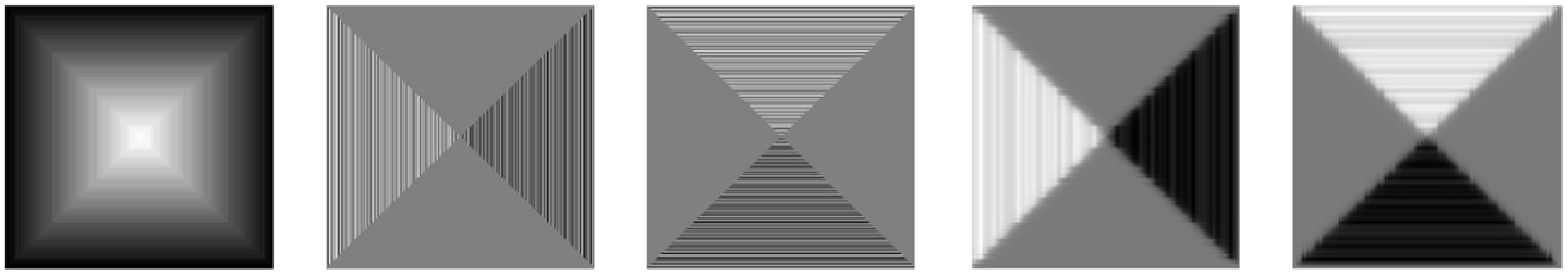
Figure 2. From the left to the right: the noised 2D pyramidal image (SNR = 0.5); the partial derivatives I_x and I_y using Horn and Schunck averaging of forward image differencing; the partial derivatives, I_x and I_y, using regularized differencing (λ = 5.0).

5. Experimental Results

This section presents various experiments on synthetic and real sequences to verify the validity of the method and its implementation. We show the recovered depth using anaglyphs (red/cyan) and color-coded displays, and novel viewpoint images. Color-coded depth is a standard display style. Anaglyphs are a convenient means for the subjective appraisal of the computed object structure. They are constructed from one of the two input images used in the experiment and the recovered depth map. Anaglyphs are best perceived on good-quality photographic paper. When viewed on standard screens, they are generally better perceived with full color resolution. Finally, we also show a novel viewpoint image, i.e., a picture of the reconstructed object as viewed from a viewpoint different from the one of either of the two input images.

For scene flow, we show a vector display of its projection from some viewpoint. Also, and since we have no ground truth of scene flow for the used sequences, we show the optical flow corresponding to it compared to the optical flow computed directly by the Horn and Schunck algorithm. We provide also a comparison to the optical flow ground truth using three kinds of error: average angular error (aae), standard angular error (stae), and endpoint error (epe). This is a good indirect way to evaluate scene flow computation results because the behavior of the Horn and Schunck method is a generally well-understood benchmark.

The formulation parameters were determined empirically. Distances are measured in pixels; the fronto-parallel plane position Z₀ has been fixed to 6 × 10⁴ pixels. The camera focal length f has been approximated to 600 pixels (Sekkati and Mitiche, 2007); the initial value of scene flow and depth at each point are, respectively, 0 and Z₀. Coefficients α and β are given in the caption of each figure. Regularized differentiation’s coefficient λ is fixed to 1 in all the examples.

In general, all of the proof-of-concept examples we show in the following support the validity of the scheme and its implementation. In the examples discussed below, one can make the following observations/conclusions:

• In all the examples, the scene flow and induced optical flow are consistent with the actual motion of the objects.

• The color-coded depth display is in line with the structure of the objects (i.e., the relative depth of object surfaces).

• The obtained optical flow is in keeping with the output of the well tested/researched benchmark algorithm of Horn and Schunck. It is worth noting here that the velocities we obtained are less noisy than those computed with Horn and Schunck algorithm. This can be explained by the fact that our method benefited from the use of (i) 3D information and (ii) better estimates of the image spatiotemporal derivatives via regularized differentiation.

• In all examples, the corresponding anaglyphs offered viewers a strong sense of depth.

5.1. Synthetic Squares Sequence

This is a sequence of two consecutive images of two overlapping squares moving against a moving background, to evaluate quantitatively the computed scene flow. This evaluation is done via the image motion that it induces. This induced motion will be compared to the actual image motion and the motion computed by the Horn and Schunck algorithm. The actual image motions are, in pixels: (−1,−1) for the upper square, (1,1) for the lower, and (0,−1) for the background. Noise has been added independently in the first and second image. Noise values are from a discretized, shifted, truncated Gaussian in the interval between 0 and 100 gray levels, within the overall range 0–255 of the image. The first of the two images is shown in the leftmost display of Figure 3; the vector-coded ground truth and the computed image motion are displayed in the second and third images, respectively; the results with the Horn and Schunck method are shown in the rightmost image. In general, such vector displays are meant to reassure that the image motion is visually consistent with its expected overall appearance. Quantitatively, the average angular error for the image motion induced by the computed scene flow is 15° and the average error on the length is 0.4 pixel. The Horn and Schunck algorithm was overwhelmed by the image noise; its average angular error is 42° and the average error on the length is 1 pixel. The proposed scheme has performed better than the Horn and Schunck algorithm because it used subsuming higher level 3D information, from which image motion can be recovered point-wise according to model Eq. 2, as well as a better estimate of the image spatiotemporal derivatives via regularized differentiation.

FIGURE 3

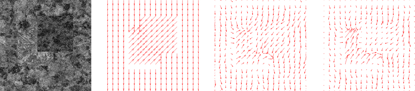
Figure 3. Synthetic squares sequence. From left to right: The first of the two images; the vector-coded ground truth; optical flow corresponding to the estimated scene flow; optical flow computed directly by the Horn and Schunck method.

5.2. Marbled-Block Sequence

In this example, we use the Marbled-block synthetic sequence from the database of KOGS/IAKS Laboratory, Germany. There are three blocks in this sequence, two of which are moving. The rightmost block moves in depth to the left and the one in the middle moves forward to the left. There are aspects, which make 3D interpretation challenging: the blocks have a macro texture of weak spatiotemporal intensity variations within the textons and similar to the texture of the floor. As a result, the occluding boundaries of the blocks are ill defined at places. The blocks also cast shadows which move. Results are shown in Figure 4. The first row depicts (from left to right): an anaglyph of the structure reconstructed from the method’s output and the first frame of the input image sequence; a color-coded display of the recovered depth along with the used color palette¹; and novel viewpoint images of the two moving blocks. Second row: a view of the scene flow vectors; optical flow corresponding to the estimated scene flow (2); the optical flow computed directly by the Horn and Schunck algorithm.

FIGURE 4

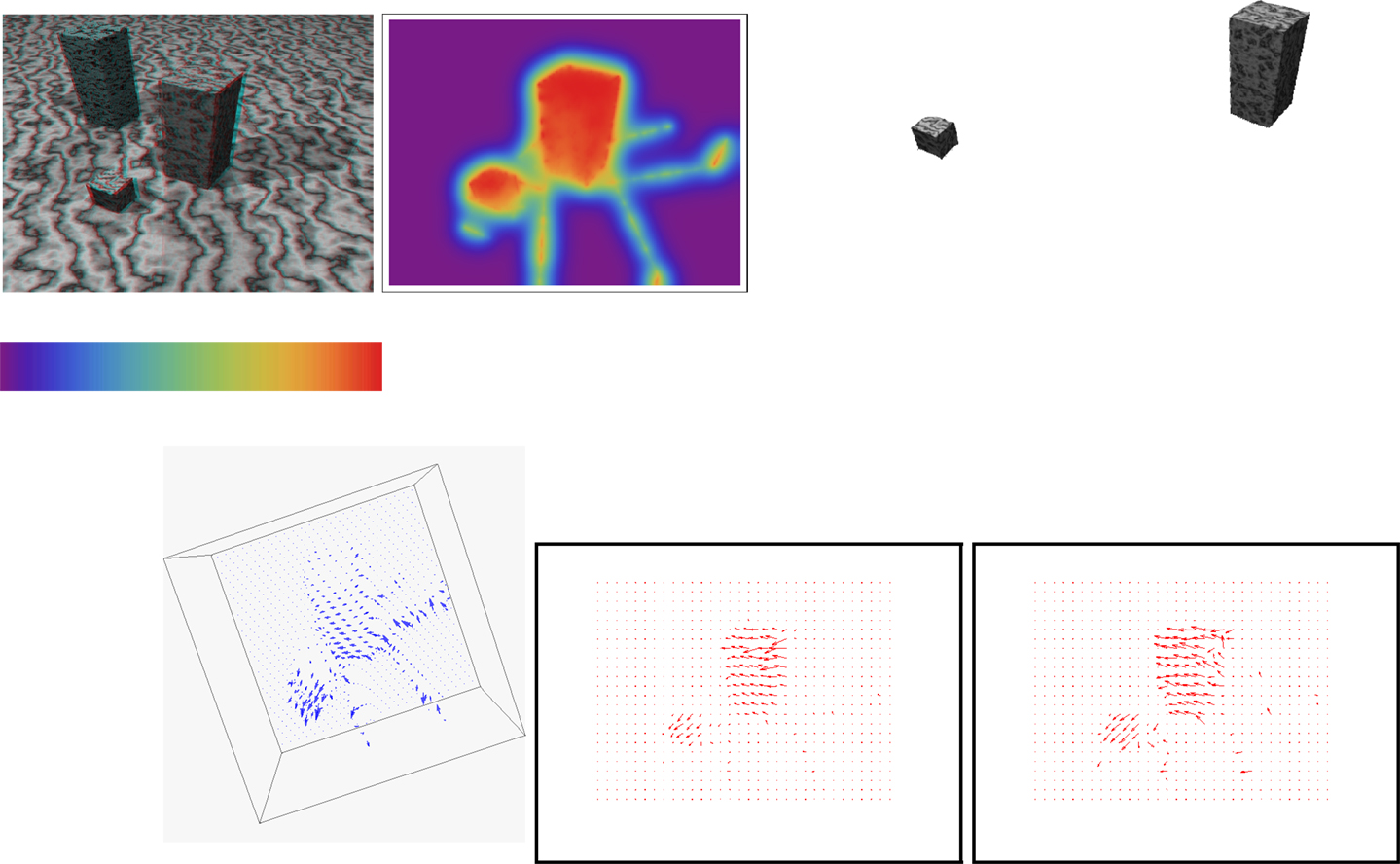
Figure 4. Marbled-blocks sequence results (better perceived when figures are enlarged on screen). Parameters: α = 6 × 10⁷ and β = 10². First row from left to right: an anaglyph of the structure reconstructed from the method’s output and the first frame of the input image sequence; a color-coded display of the recovered depth along with the used color palette, with depth increasing from right (red) to left (purple); novel viewpoint images of the two moving blocks. Second row: a view of the scene flow vectors; optical flow corresponding to the estimated scene flow (2); the optical flow computed directly by the Horn and Schunck algorithm.

5.3. Cylinder and Boxes Sequence

This second example uses a real image sequence [courtesy of Debrunner and Ahuja (1998)], shown in Figure 5. This sequence depicts three moving objects: a box moving to the right at an image rate of about 0.30 pixel per frame; a cylindrical surface rotating about a vertical axis at a velocity of one degree per frame, and moving laterally to the right at an image rate of about 0.15 pixel per frame and, finally, a flat background moving to the right (parallel to the box motion) at approximately 0.15 pixel per frame. In this example, the 3D interpretation and recovery is hard because of its unhelpful 3D motion. Results are displayed in Figure 5: first row from left to right: an anaglyph of the structure reconstructed from the method’s output and the first frame of the input image sequence; a color-coded display of the recovered depth; novel viewpoint images of the cylindrical surface and the box. Second row: a view of the scene flow vectors; optical flow corresponding to the estimated scene flow (2); the optical flow computed by the Horn and Schunck algorithm.

FIGURE 5

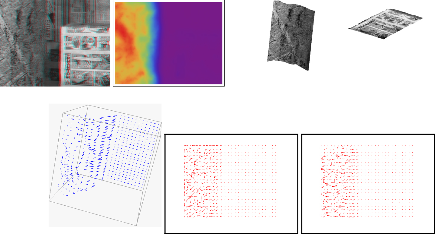
Figure 5. Cylinder and box sequence results (better perceived when figures are enlarged on screen). Parameters: α = 6 × 10⁶ and β = 10⁴. First row from left to right: an anaglyph of the structure reconstructed from the method’s output and the first frame of the input image sequence; a color-coded display of the recovered depth; novel viewpoint images the cylindrical surface and the box. Second row: a view of the scene flow vectors; optical flow corresponding to the estimated scene flow (2); the optical flow computed by the Horn and Schunck algorithm.

5.4. Berber Sequence

This example uses the Berber real sequence. The figurine rotates about a nearly vertical axis and moves forward to the left in a static environment. Figure 6 displays the results: first row from left to right: an anaglyph of the structure reconstructed from the method’s output and the first frame of the input image sequence; a color-coded display of the recovered depth; novel viewpoint images of the figurine. Second row: a view of the scene flow vectors; optical flow corresponding to the estimated scene flow (2); the optical flow computed by the Horn and Schunck algorithm.

FIGURE 6

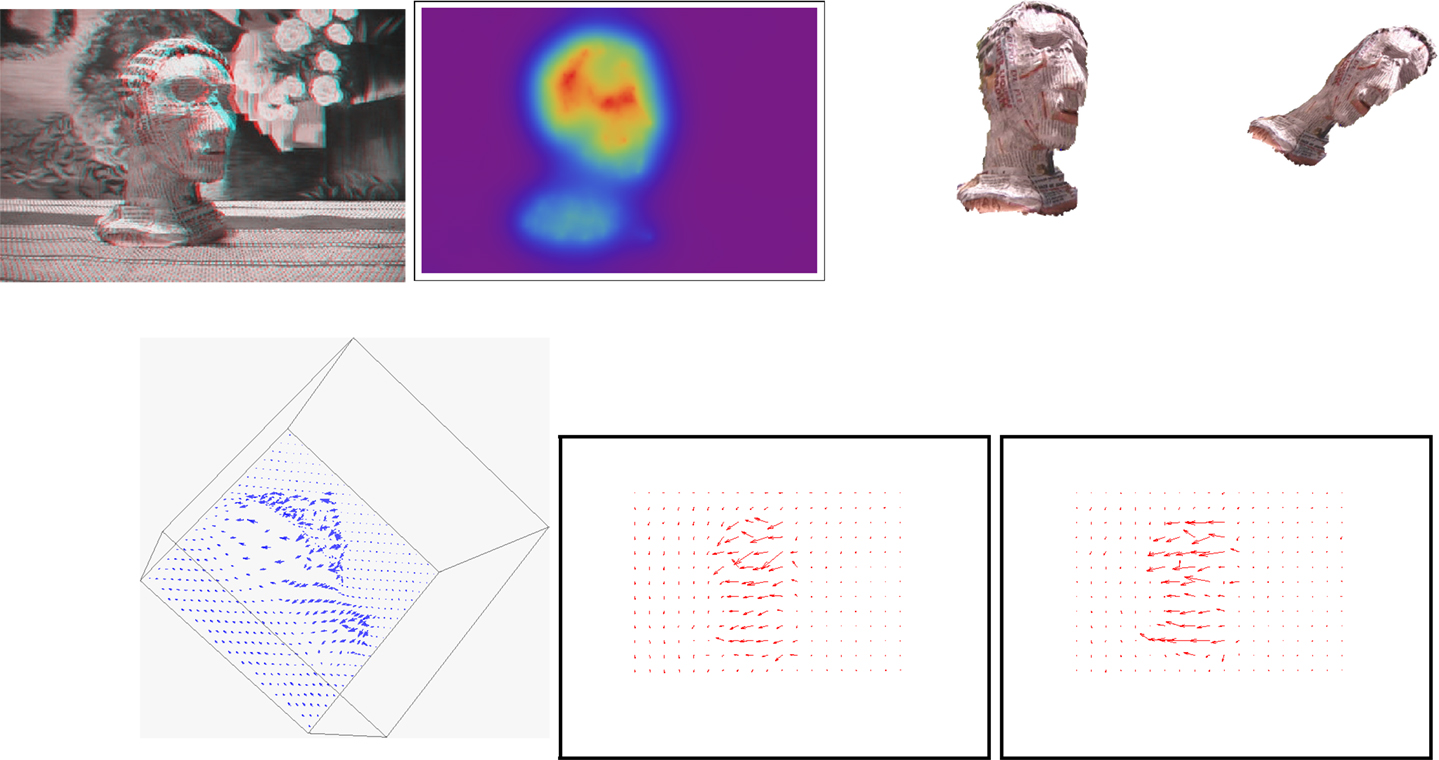
Figure 6. Berber figurine sequence results (better perceived when figures are enlarged on the screen). Parameters: α = 6 × 10⁷; β = 5 × 10⁴. First row from left to right: an anaglyph of the structure reconstructed from the method’s output and the first frame of the input image sequence; a color-coded display of the recovered depth; novel viewpoint images of the figurine. Second row: a view of the scene flow vectors; optical flow corresponding to the estimated scene flow (2); the optical flow computed by the Horn and Schunck algorithm.

5.5. Pharaohs Sequence

This example uses the Pharaohs real image sequence. There are two moving figurines in a static environment; the leftmost translates left and forward; the rightmost rotates about a nearly vertical axis to the right. Results are shown in Figure 7: first row from left to right: an anaglyph of the structure reconstructed from the method’s output and the first frame of the input image sequence; a color-coded display of the recovered depth; novel viewpoint images of the figurines. Second row: a view of the scene flow vectors; optical flow corresponding to the estimated scene flow; optical flow computed by the Horn and Schunck algorithm.

FIGURE 7

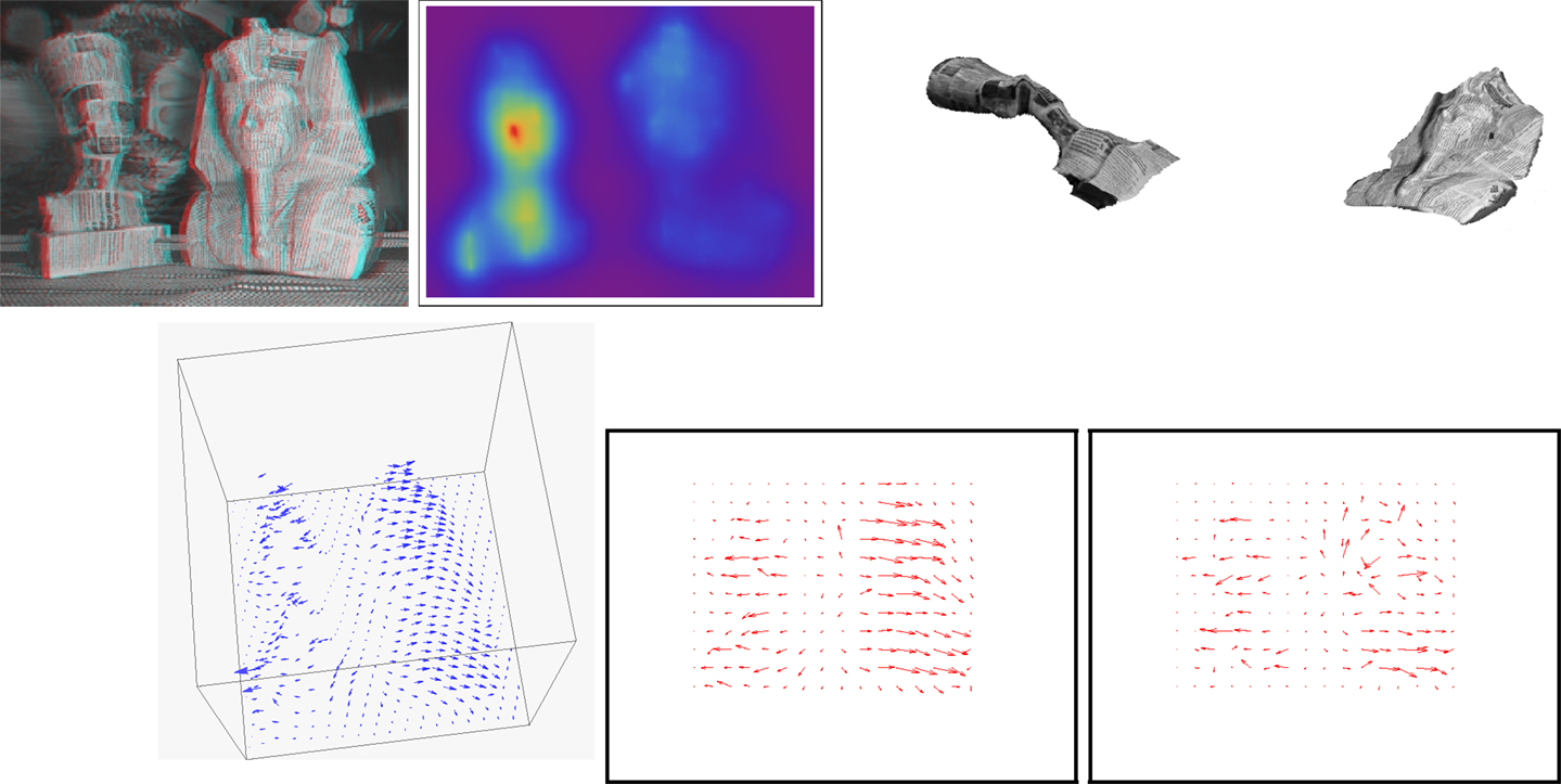
Figure 7. Pharaohs figurines sequence (better perceived when figures are enlarged on screen). Parameters: α = 6 × 10⁷; β = × 10². First row from left to right: an anaglyph of the structure reconstructed from the method’s output and the first frame of the input image sequence; a color-coded display of the recovered depth; novel viewpoint images of the figurines. Second row: a view of the scene flow vectors; optical flow corresponding to the estimated scene flow; optical flow computed by the Horn and Schunck algorithm.

The results for scene flow are shown in Table 1 for each of the examples described above.

TABLE 1

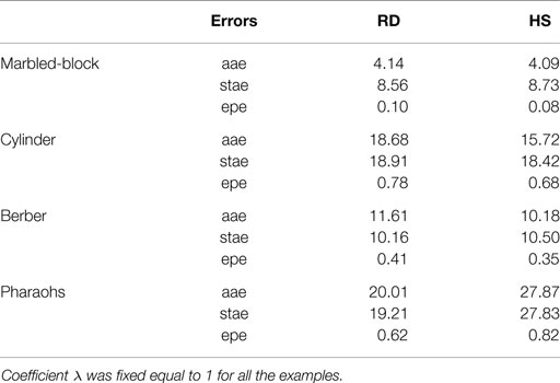
Table 1. Average angular error (aae), standard angular error (stae), and endpoint error (epe) for the optical flow corresponding to the estimated scene flow using regularized differentiation (RD) vs. optical flow computed directly by the Horn and Schunck algorithm (HS).

6. Conclusion and Discussion

The goal of this study was concurrent recovery of scene flow and depth from a monocular image sequence. We developed a variational method, which minimizes a functional containing a data term of joint scene flow and depth conformity to the image sequence spatiotemporal variations, and quadratic smoothness regularization terms. The data term follows rewriting optical flow as a function of scene flow and depth in the classical optical flow gradient constraint of Horn and Schunck. As a result, the formulation is analogous to the classical Horn and Schunck optical flow estimation method, except that it involves the variables of scene flow and depth rather than image motion. Monocular processing is a unique feature of this scheme because previous scene flow recovery schemes have used binocular image sequences rather than a single image stream as in this study.

Another characteristic is the occurrence of both depth and scene flow as unknowns in the equations used to state the problem. The variational paradigm fitted naturally with these equations to give a single optimization formulation, free from the intervention of outside processes since all the relevant variables, namely depth and scene flow coordinates, occur simultaneously. As a result, the formulation translates into a tractable algorithm whose behavior can be explained. This algorithm follows the discretization of the objective functional Euler–Lagrange equations, giving a large scale sparse system of linear equations in the unknowns of depth and the three scene flow coordinates. The equations can be ordered in such a way that its matrix is symmetric positive definite such that they can be solved efficiently by Gauss–Seidel iterations.

The focus of this study being on the formulation proper, it was sufficient to use Gauss–Seidel iterations in the proof-of-concepts examples that we described in the experimental section. However, one can explore other schemes for more efficient numerical resolution as the literature on large sparse systems of linear equations is quite vast. For instance, one can investigate (Ciarlet, 1982) classical convergence acceleration of the Gauss–Seidel by successive over-relaxation, or an iterative scheme designed for positive definite systems, such as the conjugate gradient algorithm. The sequential subspace correction (SSC) method (Hackbush, 1994), which would process the minimization in the four independent linear subspaces of depth and scene flow coordinates sequentially can also prove to be quite efficient; for each subspace, the Gauss–Seidel iterations can be used. The SSC can be parallelized. There is also a rich literature on efficient modern Krylov subspace methods where a matrix need only be specified as a matrix–vector operator (Simoncini and Szyld, 2007).

This study used Tikhonov regularization for scene flow and depth. It did not affect the purpose of formulating monocular recovery of these variables. However, quadratic regularization smooths the variables recovered at and in the proximity of their discontinuities, namely sharp changes in depth and motion boundaries. There are several ways of specifying boundary preserving recovery (Mitiche and Aggarwal, 2013). For instance, one can use the Aubert et al. function, in place of the quadratic function, or simply the L¹ norm. In addition to preserving discontinuities, the L¹ norm can be approximated in practice for faster computation without affecting accuracy in a noticeable way. Both motion and depth discontinuities can also be preserved by concurrent motion computation and segmentation (Mitiche and Sekkati, 2006).

The examples we gave are for proof of concept only. They show that the formulation is sound, correctly implemented, but has obvious limitations, such as boundary blurring interpretation and use of approximate camera parameters. Nevertheless, the results clearly indicate that the method is worthy of further investigation. We are currently extending it to account for motion and depth discontinuities via L¹ regularization. We are also investigating joint motion segmentation and estimation, an extension to scene flow and depth of the scheme in (Mitiche and Sekkati, 2006). Experimental validation must be based on a larger database of three-dimensional moving objects of various geometries that would test various difficulties, such as motion and depth discontinuities, motion of large extent, and image noise and resolution in common practical settings. In particular, quantitative validation will require computer graphics generation of appropriate synthetic objects in motion for which ground truth scene flow can be calculated.

Conflict of Interest Statement

The authors declare that the research was conducted in the absence of any commercial or financial relationships that could be construed as a potential conflict of interest.

Footnote

1. ^We used the same color palette for all examples, with depth increasing from right (red) to left (purple)

References

Adiv, G. (1985). Determining three-dimensional motion and structure from optical flow generated by several moving objects. IEEE Trans. Pattern Anal. Mach. Intell. 7, 384–401. doi: 10.1109/TPAMI.1985.4767678

PubMed Abstract | CrossRef Full Text | Google Scholar

Aubert, G., Deriche, R., and Kornprobst, P. (1999). Computing optical flow via variational techniques. SIAM J. Appl. Math. 60, 156–182. doi:10.1137/S0036139998340170

CrossRef Full Text | Google Scholar

Basha, T., Moses, Y., and Kiryati, N. (2013). Multi-view scene flow estimation: a view centered variational approach. Int. J. Comput. Vis. 101, 6–21. doi:10.1007/s11263-012-0542-7

CrossRef Full Text | Google Scholar

Brodsky, T., Fermuller, C., and Aloimonos, Y. (2000). Structure from motion: beyond the epipolar constraint. Int. J. Comput. Vis. 37, 231–258. doi:10.1023/A:1008132107950

CrossRef Full Text | Google Scholar

Bruss, A. R., and Horn, B. K. P. (1983). Passive navigation. Comput. Vis. Graph. Image Process. 21, 3–20. doi:10.1016/S0734-189X(83)80026-7

CrossRef Full Text | Google Scholar

Chartrand, R. (2005). Numerical Differentiation of Noisy, Nonsmooth Data. Los Alamos National Laboratory.

Google Scholar

Ciarlet, P. (1982). “Introduction à l’analyse numérique matricielle et à l’optimisation,” in Collection Mathématiques appliquées pour la maîtrise (Masson).

Google Scholar

Cullum, J. (1971). Numerical differentiation and regularization. SIAM J. Numer. Anal. 8, 254–265. doi:10.1137/0708026

CrossRef Full Text | Google Scholar

De Micheli, E., and Giachero, F. (1994). “Motion and structure from one dimensional optical flow,” in Computer Vision and Pattern Recognition, 1994. Proceedings CVPR ‘94., 1994 IEEE Computer Society Conference on (Seatle, WA: IEEE), 962–965.

Google Scholar

Debrunner, C., and Ahuja, N. (1998). Segmentation and factorization-based motion and structure estimation for long image sequences. IEEE Trans. Pattern Anal. Mach. Intell. 20, 206–211. doi:10.1109/34.659941

CrossRef Full Text | Google Scholar

Deriche, R., Kornprobst, P., and Aubert, G. (1995). “Optical-flow estimation while preserving its discontinuities: a variational approach,” in ACCV, Volume 1035 of Lecture Notes in Computer Science, eds S. Z. Li, D. P. Mital, E. K. Teoh, and H. Wang (Singapore: Springer), 71–80.

Google Scholar

Fejes, S., and Davis, L. S. (1998). “What can projections of flow fields tell us about visual motion,” in ICCV (Bombay: IEEE), 979–986.

Google Scholar

Forsythe, G. E., Malcolm, M. A., and Moler, C. B. (1977). “Computer methods for mathematical computations,” in Prentice-Hall Series in Automatic Computation (Englewood Cliffs, NJ: Prentice-Hall).

Google Scholar

Gupta, N., and Kanal, N. (1995). 3-D motion estimation from motion field. Artif. Intell. 78, 45–86. doi:10.1016/0004-3702(95)00031-3

CrossRef Full Text | Google Scholar

Hackbush, W. (1994). Iterative Solution of Large Sparse Systems of Equations, Vol. 95. Springer.

Google Scholar

Hanke, M., and Scherzer, O. (2001). Inverse problems light: numerical differentiation. Am. Math. Mon. 108, 512–521. doi:10.2307/2695705

CrossRef Full Text | Google Scholar

Heeger, D. J., and Jepson, A. D. (1992). Subspace methods for recovering rigid motion I: algorithm and implementation. Int. J. Comput. Vis. 7, 95–117. doi:10.1007/BF00128130

CrossRef Full Text | Google Scholar

Hildreth, E. C. (1984). The Measurement of Visual Motion. PhD thesis, Massachusetts Institute of Technology, Cambridge, MA; London.

Google Scholar

Horn, B. K. P., and Schunck, B. G. (1981). Determining optical flow. Artif. Intell. 17, 185–203. doi:10.1016/0004-3702(81)90024-2

CrossRef Full Text | Google Scholar

Horn, B. K. P., and Weldon, E. J. (1988). Direct methods for recovering motion. Int. J. Comput. Vis. 2, 51–76. doi:10.1007/BF00836281

CrossRef Full Text | Google Scholar

Huguet, F., and Devernay, F. (2007). “A variational method for scene flow estimation from stereo sequences,” in IEEE International Conference on Computer Vision (ICCV) (Rio de Janeiro: IEEE), 1–7.

Google Scholar

Hung, Y. S., and Ho, H. T. (1999). A Kalman filter approach to direct depth estimation incorporating surface structure. IEEE Trans. Pattern Anal. Mach. Intell. 21, 570–575. doi:10.1109/34.771330

CrossRef Full Text | Google Scholar

Liu, H., Chellappa, R., and Rosenfeld, A. (2002). “A hierarchical approach for obtaining structure from two-frame optical flow,” in Proceedings of the Workshop on Motion and Video Computing, MOTION ‘02 (Washington, DC: IEEE Computer Society), 214–219.

Google Scholar

Longuet-Higgins, H. C., and Prazdny, K. (1980). The interpretation of a moving retinal image. Proc. R. Soc. Lond. B Biol. Sci. 208, 385–397. doi:10.1098/rspb.1980.0057

PubMed Abstract | CrossRef Full Text | Google Scholar

MacLean, W. J., Jepson, A. D., and Frecker, R. C. (1994). “Recovery of egomotion and segmentation of independent object motion using the em algorithm,” in British Machine Vision Conference, BMVC, ed. E. R. Hancock (New York, UK: BMVA Press), 1–10.

Google Scholar

Mitiche, A., and Aggarwal, J. (2013). Computer Vision Analysis of Image Motion by Variational Methods. Springer.

Google Scholar

Mitiche, A., and Hadjres, S. (2003). Mdl estimation of a dense map of relative depth and 3D motion from a temporal sequence of images. Pattern Anal. Appl. 6, 78–87. doi:10.1007/s10044-002-0182-6

CrossRef Full Text | Google Scholar

Mitiche, A., and Sekkati, H. (2006). Optical flow 3D segmentation and interpretation: a variational method with active curve evolution and level sets. IEEE Trans. Pattern Anal. Mach. Intell. 28, 1818–1829. doi:10.1109/TPAMI.2006.232

PubMed Abstract | CrossRef Full Text | Google Scholar

Pons, J.-P., Keriven, R., Faugeras, O., and Hermosillo, G. (2003). “Variational stereovision and 3d scene flow estimation with statistical similarity measures,” in IEEE International Conference On Computer Vision (ICCV) (Nice: IEEE), 597–602.

Google Scholar

Rabe, C., Müller, T., Wedel, A., and Franke, U. (2010). “Dense, robust, and accurate motion field estimation from stereo image sequences in real-time,” in Proceedings of the 11th European Conference on Computer Vision, Volume 6314 of Lecture Notes in Computer Science, eds K. Daniilidis, P. Maragos, and N. Paragios (Heraklion: Springer), 582–595.

Google Scholar

Reinsch, C. H. (1967). Smoothing by spline functions. Numerische Mathematik 10, 177–183. doi:10.1007/BF02162161

CrossRef Full Text | Google Scholar

Schoenberg, I. J. (1964). Spline functions and the problem of graduation. Proc. Natl. Acad. Sci.U.S.A. 54, 947–950. doi:10.1073/pnas.52.4.947

CrossRef Full Text | Google Scholar

Sekkati, H., and Mitiche, A. (2006a). Concurrent 3-D motion segmentation and 3-D interpretation of temporal sequences of monocular images. IEEE Trans. Image Process. 15, 641–653. doi:10.1109/TIP.2005.863699

PubMed Abstract | CrossRef Full Text | Google Scholar

Sekkati, H., and Mitiche, A. (2006b). Joint optical flow estimation, segmentation, and 3D interpretation with level sets. Comput. Vis. Image Underst. 103, 89–100. doi:10.1016/j.cviu.2005.11.002

CrossRef Full Text | Google Scholar

Sekkati, H., and Mitiche, A. (2007). A variational method for the recovery of dense 3D structure from motion. Rob. Auton. Syst. 55, 597–607. doi:10.1016/j.robot.2006.11.006

PubMed Abstract | CrossRef Full Text | Google Scholar

Shahraray, B., and Brown, M. (1988). “Robust depth estimation from optical flow,” in International Conference on Computer Vision, ICCV (Tampa, FL: IEEE), 641–650.

Google Scholar

Simoncini, V., and Szyld, D. B. (2007). Recent computational developments in Krylov subspace methods for linear systems. Numer. Lin. Algebra Appl. 14, 1–59. doi:10.1002/nla.499

CrossRef Full Text | Google Scholar

Srinivasan, S. (2000). Extracting structure from optical flow using the fast error search technique. Int. J. Comput. Vis. 37, 203–230. doi:10.1023/A:1008111923880

CrossRef Full Text | Google Scholar

Stoer, J., and Bulirsch, R. (2002). Introduction to Numerical Analysis. Texts in Applied Mathematics; 12, 3rd Edn. New York, NY: Springer.

Google Scholar

Taalebinezhaad, M. A. (1992). Direct recovery of motion and shape in the general case by fixation. IEEE Trans. Pattern Anal. Mach. Intell. 14, 847–853. doi:10.1109/34.149584

CrossRef Full Text | Google Scholar

Terzopoulos, D. (1986). Regularization of inverse visual problems involving discontinuities. IEEE Trans. Pattern Anal. Mach. Intell. 8, 413–424. doi:10.1109/TPAMI.1986.4767807

CrossRef Full Text | Google Scholar

Ullman, S. (1983). Computational Studies in the Interpretation of Structure and Motion: Summary and Extension. Technical Report, MIT.

Google Scholar

Vedula, S., Baker, S., Rander, P., Collins, R., and Kanade, T. (2005). Three-dimensional scene flow. IEEE Trans. Pattern Anal. Mach. Intell. 27, 475–480. doi:10.1109/TPAMI.2005.63

PubMed Abstract | CrossRef Full Text | Google Scholar

Vogel, C., Schindler, K., and Roth, S. (2013). “Piecewise rigid scene flow,” in IEEE International Conference on Computer Vision, ICCV 2013 (Sydney, NSW: IEEE), 1377–1384.

Google Scholar

Vogel, C. R. (2002). Computational Methods for Inverse Problems. SIAM Frontiers in Applied Mathematics.

Google Scholar

Weber, J., and Malik, J. (1997). Rigid body segmentation and shape description from dense optical flow under weak perspective. IEEE Trans. Pattern Anal. Mach. Intell. 19, 139–143. doi:10.1109/34.574794

CrossRef Full Text | Google Scholar

Wedel, A., Brox, T., Vaudrey, T., Rabe, C., Franke, U., and Cremers, D. (2011). Stereoscopic scene flow computation for 3D motion understanding. Int. J. Comput. Vis. 95, 29–51. doi:10.1007/s11263-010-0404-0

CrossRef Full Text | Google Scholar

Wedel, A., Rabe, C., Vaudrey, T., Brox, T., Franke, U., and Cremers, D. (2008). “Efficient dense scene flow from sparse or dense stereo data,” in European Conference on Computer Vision (ECCV), Vol. 1 (Marseille: Springer), 739–751.

Google Scholar

Xiong, Y., and Shafer, S. (1995). Dense Structure from a Dense Optical Flow. Technical Report CMU-RI-TR-95-10. Pittsburgh, PA: Robotics Institute.

Google Scholar

Zhang, Y., and Kambhamettu, C. (2000). “Integrated 3D scene flow and structure recovery from multiview image sequences,” in IEEE Conference on Computer Vision and Pattern Recognition (CVPR), Vol. 2 (Hilton Head, SC: IEEE), 674–681.

Google Scholar