An evaluation of streaming algorithms for distinct counting over a sliding window

1. Introduction

Let S be a stream of identifiers, each chosen from a universe U. We consider the problem of maintaining the number of distinct identifiers in S in a single pass through S using limited memory, a problem we henceforth refer to as “distinct counting.” Distinct counting is a fundamental problem in databases with a wide variety of applications in database query processing and optimization (Selinger et al., 1979; Youssefi and Wong, 1979; Whang et al., 1981, 1990; Gelenbe and Gardy, 1982) and network monitoring (Tosun, 2007; Lahiri et al., 2011; Singh and Tirthapura, 2014) and is one of the earliest problems studied in the area of streaming algorithms.

An example application of distinct counting in network monitoring is to track the number of distinct network connections established by a source IP address. Tracking sources that establish a large number of distinct connections can help identify network anomalies such as worm propagation and DDoS attacks (Venkataraman et al., 2005). Since a network monitor has to simultaneously monitor a number of sources, it cannot afford to use much memory for each source and needs a small-space data structure for counting the number of distinct identifiers per source. Further, it is necessary to count the number of distinct identifiers within a subsequence of the stream consisting of the most recently observed elements, commonly modeled using a “sliding window” in the stream. Aggregation over a sliding window arises naturally in real-time monitoring situations such as network traffic engineering, telecom analytics, and cyber security (e.g., Datar et al., 2002; Gibbons and Tirthapura, 2002; Golab et al., 2003; Tirthapura et al., 2006; Braverman and Ostrovsky, 2007; Busch and Tirthapura, 2007; Fusy and Giroire, 2007). For instance, in network traffic engineering (Fraleigh et al., 2000), current network performance is monitored over a sliding window to adjust the bandwidth of the network dynamically.

A time-based sliding window of length T is defined as the set of the stream elements that have arrived within the last T time units, for some parameter T. The abstraction of a sliding window is well accepted today and has found its way into the query processing interface of major stream-processing systems, including IBM Infosphere Streams (Nasgaard et al., 2009) and Apache Spark Streaming (Zaharia et al., 2013). For instance, in IBM Infosphere Streams, it is possible to apply each streaming aggregation operator (including distinct counting) over a sliding window. In this work, we consider the efficient implementation of distinct counting over a sliding window of a stream.

From a theoretical perspective, distinct counting is widely studied (e.g., Flajolet and Martin, 1985; Flajolet, 1990; Whang et al., 1990; Haas et al., 1995; Alon et al., 1996; Charikar et al., 2000; Gibbons and Tirthapura, 2001; Bar-Yossef et al., 2002; Durand and Flajolet, 2003; Woodruff, 2004; Fusy and Giroire, 2007; Gibbons, 2007; Chen and Cao, 2009; Giroire, 2009; Kane et al., 2010). However, there has not been much attention to engineering a good implementation. Most current algorithms for distinct counting over a stream (e.g., Flajolet and Martin, 1985; Whang et al., 1990; Haas et al., 1995; Alon et al., 1996; Charikar et al., 2000; Gibbons and Tirthapura, 2001; Bar-Yossef et al., 2002; Durand and Flajolet, 2003; Woodruff, 2004; Fusy and Giroire, 2007; Giroire, 2009; Kane et al., 2010) have been designed for the case of “infinite window,” where the scope of aggregation is all the elements seen so far. There have been some algorithms designed for a sliding window (e.g., Datar et al., 2002; Gibbons and Tirthapura, 2002; Zhang et al., 2010), but so far, there has not been a comprehensive evaluation and comparison of different approaches.

We present the first detailed experimental evaluation of algorithms for distinct counting over a sliding window. We consider prominent algorithms and evaluate them with respect to their memory consumption, processing time, query time, and accuracy. In some cases that we considered, it was known previously how to extend the algorithm to a sliding window, while in other cases, we design an extension to a sliding window of a distinct counting algorithm originally designed for the infinite window. We set out to answer the following questions.

• How do different algorithms compare in terms of accuracy and processing time, given the same amount of main memory?

• Most algorithms for distinct counting work as follows. They first design a “rough” estimator whose output is a random variable, but whose error can be large. Then, many such estimators are aggregated in order to improve the accuracy. A few different methods are used for boosting accuracy, including “median-of-many,” “split-and-add,” and “stochastic averaging”; these methods are described in Section 2. Which aggregation method is suitable for each algorithm?

• Every algorithm known for distinct counting uses a hash function that maps input identifiers, which maybe non-uniformly distributed within the input universe, to another universe, where they are uniformly distributed. The hash function has a significant impact on the accuracy and the runtime. Which hash function gives the best performance? We compared five popular hash functions, MurmurHash,¹ Jenkins Hash,² modulo congruential hash, Fowler-Noll-Vo (FNV)³ hash and the Secure Hash Algorithm 1 (SHA-1)⁴.

• How is the performance of an algorithm affected by the relative frequencies of queries (for the number of distinct elements) versus element arrivals?

We consider the following prominent algorithms: Probabilistic Counting with Stochastic Averaging (PCSA) (Flajolet and Martin, 1985; Datar et al., 2002), Randomized Wave (RW) (Gibbons and Tirthapura, 2002), Linear Counting (LC) (Whang et al., 1990), Durand-Flajolet (DF, also known as “Loglog” in the literature) (Durand and Flajolet, 2003), and the first algorithm due to Bar-Yossef et al. (2002), which we call BJKST1. Among these, RW is the only algorithm which was designed for distinct counting over a sliding window. Though PCSA was originally designed for an infinite window, an extension to a sliding window was described in Datar et al. (2002). For the rest of the algorithms, LC, DF, and BJKST1, we present an extension for the case of a sliding window. We discuss these algorithms in greater detail in Section 2.1.

1.1. Summary of Results

1.1.1. Accuracy

Given equal memory on the same dataset, we observed that the Randomized Wave (RW) consistently produces the most accurate estimate, followed by PCSA and then BJKST1. We also observe that Linear Counting (LC) performs with good accuracy when the memory allotted is large relative to the number of distinct elements within a sliding window; when the memory allotted is smaller, LC is unable to produce a reasonable estimate.

1.1.2. Runtime

When the frequency of updates (element arrivals) is much larger than the frequency of queries, PCSA and DF are the fastest algorithms, followed by RW and BJKST1. However, if the frequency of queries increases, then the runtimes of PCSA, DF, and LC increase significantly, and RW and BJKST1 are the fastest algorithms.

1.1.3. Hash Function

We found that all algorithms consistently give the most accurate estimates when MurmurHash is used as the hash function. Fortunately, it is also the fastest of all five hash functions that we considered, so that MurmurHash is unambiguously the best hash function among those we considered. While the accuracy of Jenkins hash is close to MurmurHash, it is slower than MurmurHash. The popular modulo congruential hash function performs much worse than MurmurHash and Jenkins hash, in terms of accuracy.

1.1.4. Accuracy Boosting Method

We observed that PCSA and DF work best with stochastic averaging. This is to be expected, since PCSA and DF were designed with stochastic averaging in mind. Surprisingly, we found that the remaining algorithms (LC, RW, and BJKST1) performed with the smallest average error when the entire space is allotted to a single instance of the algorithm, with no further boosting of accuracy.

Note that our comparison keeps the total space fixed for different accuracy boosting methods. For instance, if we used the median of five estimators as our accuracy boosting method, then the space allocated to each instance of the algorithm is only a fifth of the total space. Thus, our results do not contradict earlier results due to Bar-Yossef et al. (2002) and Gibbons and Tirthapura (2002), who advocate using the median-of-many estimators. Their observation is that the probability of being inaccurate can be reduced by taking the median-of-many estimators, at the expense of greater space. Our experiments show that if space is held fixed, then the smallest average error is achieved when the entire space (memory) is given to a single estimator.

Overall, if accuracy is the most important criterion, then RW performs best. RW is also the fastest algorithm when the rate of updates is low relative to the rate of queries (approximately <100 updates per query). PCSA is the best choice if processing time is the most important criterion, and the rate of querying is not very frequent.

1.1.5. Relation to Prior Work

Prior work on experimental evaluations of distinct counting include Astrahan et al. (1987), Estan et al. (2006), Metwally et al. (2008), and Resvanis and Chatzigiannakis (2009), who compare the performance of different algorithms for distinct counting, such as PCSA and Linear Counting, over an infinite window. The most detailed comparison for distinct counting algorithms over infinite window seems to be due to Metwally et al. (2008), who grouped the algorithms into different categories: Logarithmic Hashing, e.g., PCSA (Flajolet and Martin, 1985); Interval-based, e.g., BJKST1 (Bar-Yossef et al., 2002); Pure Bucket-based, e.g., Linear Counting (Whang et al., 1990); Hybrid Bucket Sampling, e.g., Distinct Sampling (Gibbons and Tirthapura, 2001); Hybrid Bucket Logarithmic, e.g., Multiresolution Bitmap (Estan et al., 2006); and concluded that Linear Counting is overall the best algorithm, both in terms of accuracy and runtime.

Our work differs from that of Metwally et al. (2008) in the following ways. Mainly, we consider aggregation over a sliding window while they consider aggregation over an infinite window. The algorithms involved are different, and the results that we obtain are also different. In particular, we observe that Linear Counting (LC) does not perform very well over a sliding window. The accuracy of LC over a sliding window is very inconsistent for our datasets when the memory used is <1,000–2,000 KB; in some cases, it does not even produce an estimate. In contrast, the accuracy of RW and PCSA is consistently within 1%, even when the total memory is <1,000 KB. The difference in results between the sliding window case and the infinite window case is because the sliding window data structure needs to maintain a timestamp (of expiry) for each bit in the data structure maintained by LC. This overhead significantly increases the space required by LC to maintain an estimate of the distinct count and consequently decreases its accuracy for a given space budget. In addition, our evaluation considers important decisions, such as the choice of hash function, and the accuracy boosting method. All implementations in Metwally et al. (2008) used the modulo congruential hash function; our experiments show that other hash functions perform much better. Furthermore, different accuracy boosting methods are not explored. The size of datasets that we consider (up to 100 million distinct elements) is much larger than in the experiments of Metwally et al. (2008) (∼2 million distinct elements).

2. Materials and Methods

There are two types of sliding windows commonly considered, count-based window and time-based window. A count-based window of size W is the set of the W most recent elements in the stream. A time-based window of size T is the set of all stream elements that have arrived within the T most recent time units. We consider a time-based window, since a count-based window is a special case of a time-based window. An algorithm for a time-based window can also be used for a count-based window by setting the timestamp to be equal to the stream position.

2.1. Algorithms

We present an overview of the algorithms that we consider. For the following discussion, we assume that the domain of elements is [N] = {1, 2, .…, N}, and that N is a power of 2. Each element of the stream is a tuple (e, t), where e ∈ [N] and t ≥ 0 is an integer timestamp. We assume that timestamps are in a non-decreasing order, but not necessarily consecutive. When a query is posed at time t, the requirement is to estimate the number of distinct elements within a timestamp based sliding window of size T, i.e., those elements with timestamps r such that (t − T + 1) ≤ r ≤ t.

2.1.1. Probabilistic Counting with Stochastic Averaging

We recall the PCSA algorithm for an infinite window (Flajolet and Martin, 1985). The algorithm maintains a bit vector B of size log₂ N. It uses a hash function h: [N] → {1, 2, …, log₂ N}, such that for each e ∈ [N], and b ∈ {1, 2, …, log₂ N}, Pr [h(e) = b] = 2^−b. Initially, all bits of B are set to 0. When an element e arrives, B[h(e)] is set to 1. The intuition is that approximately 2ⁱ distinct elements must be seen before B[i] is set to 1. When there is a query for the number of distinct elements, the bits of B are scanned from position 1 onward, to find the index of the lowest bit x that is not set. The estimate returned is 1.29281 × 2^x+1.

To adapt this to a sliding window, we use ideas from Datar et al. (2002) and Zhang et al. (2010). Instead of a bit vector B, we use a vector M of length log₂ N, indexed from 1 till log₂ N, to store timestamps. Initially, all entries of M are set to 0. When an element (e, t) arrives, M[h(e)] is set to t. Note that M[i] tracks the latest timestamp at which an element hashes to index i. When there is a query for the number of distinct elements within a time-based sliding window of size T, the algorithm scans M to find the smallest index x such that either M[x] is 0, or the timestamp of x has expired, i.e., M[x] < (t − T + 1), where t is the current time. The estimate returned is 1.29281 × 2^x+1, as before.

We implement an enhancement of the above basic scheme, based on stochastic averaging (PCSA), also proposed in Flajolet and Martin (1985). In PCSA, k copies of the above data structure are used. Input elements are first partitioned into k non-overlapping groups, using a hash function g; an element (e, t) is forwarded to one of the k data structures, according to g(e). The final estimate is $1.29281\times k\times 2^{\widehat{x}+1}$, where $\widehat{x}$ is the average of the individual xs obtained from the k different data structures. Similar to PCSA for an infinite window, the processing time per element of PCSA for a sliding window is O(1), and the query time is O(k log N). Suppose that a timestamp can be stored in $\mathcal{T}$ bits. The space taken by the sliding window version is O($\mathcal{T}$ k log N) bits, which is a factor Θ($\mathcal{T}$) larger than the infinite window version which takes O(k log N) bits of space.

AMS, due to Alon et al. (1996) is another algorithm for distinct counting for an infinite window, with the same intuition as PCSA. Though AMS provides a cleaner theoretical guarantee than PCSA, PCSA has been found to be more accurate in practice than AMS, for example, as in the evaluation by Gibbons (2007).

2.1.2. Linear Counting

Linear Counting, due to Whang et al. (1990), uses a bit vector B of size n = D_max/ρ, where D_max is an upper bound on the maximum number of distinct elements in the data stream, and ρ is a constant called the “load factor.” The algorithm uses a hash function h: [N] → {1, 2, …, N} such that for each e ∈ [N], and b ∈ {1, 2, …, n}, Pr [h(e) = b] = 1/n. Initially, all bits in B are set to 0. Each element e of the data stream is uniformly and independently hashed to an index in the bit vector, and the corresponding bit is set to 1. When a query is made, the number of distinct elements is estimated as m ln (n/m) where m is the number of bits in B that are still 0. Whang et al. (1990) show that accurate estimates can be obtained when ρ ≤ 12. However, when ρ is significantly >12, the estimates are poor due to a large density of 1s in the bit array.

We extend the above to a sliding window as follows. Instead of a bit vector, we use a vector of timestamps, M, of size n, indexed from 1 till n. When element (e, t) arrives, M[h(e)] is set to t. When a query is made for the number of distinct elements within the window, the entire vector M is scanned and the number of indices that either have value 0 or whose timestamps have expired is used instead of m in the above formula. Note that the processing time per element is O(1) and the time to answer a query is O(n), which is expensive since n is linear in the number of distinct elements. The total time is still reasonable if the frequency of queries is small when compared with the frequency of updates (infrequent queries), but poor if queries are more frequent.

For the case of frequent queries, we modified LC by introducing a data structures in addition to M – a list L that comprises of tuples of the form (t, a) and is ordered according to t, the time stamp of observation, and a is the value to which the element hashes to. In the vector M, in addition to a timestamp t, there is also a pointer to the occurrence of t in L, so that if an element with a new timestamp hashes to an index in M, the corresponding entry with older timestamp is deleted from the list, and the newer entry with current timestamp is made at the head.

The modified version of LC, which we call “LC2,” requires not only 2$\mathcal{T}$ bytes to maintain two copies of timestamp per index of M but also an overhead for maintaining an list, which can be twice the pointer size in a typical implementation such as the C++ Standard Template Library. The expired timestamp is determined from the tail of L in constant time. A single variable can keep track of the number of indexes with expired timestamps or with an initial value of zero. When a query is posed, the number of relevant bits can be determined in O(1) time. Overall, we get O(1) time for update as well as a query, but at the cost of a significant space overhead. A significant drawback of LC is that ρ cannot exceed 12 (Whang et al., 1990), so that the space used by the algorithm is at least D_max/12. The accuracy of the estimate falls drastically as ρ increases.

2.1.3. BJKST1

BJKST1 is the first algorithm in Bar-Yossef et al. (2002). We first describe the infinite window version and then present an adaptation to a sliding window. Each stream element is hashed uniformly using a function h: [N] → [N³]. At each instant the algorithm maintains the τ smallest hash outputs, for some τ that depends on the desired accuracy. When a query is posed, an estimate of distinct count is returned as τN³/v_τ, where v_τ is the τth smallest hash output.

We propose the following adaptation to the sliding window. We associate with each value among the τ smallest hash outputs, a timestamp equal to the most recent time when this value was observed. It is not possible to maintain τth minimum of hash outputs exactly in a sliding window using a bounded space for a fixed value of τ (as discussed in Datar et al. (2002), maintaining the minimum over a sliding window requires linear space in the worst case). So we vary the value of τ so that the algorithm uses a bounded space to estimate distinct count. As the hash outputs of data elements are generated randomly, the algorithm uses an expected space cost of O(log N/ε²) to estimate distinct count, where we set the maximum value of τ to a constant θ which depends on the space allocated to the algorithm. Our idea is influenced by the algorithm for computing minimum element over a sliding window in Datar et al. (2002) and Fusy and Giroire (2007).

We maintain a list L of (h(e), t) tuples, where e is the element ID observed at timestamp t. When a new element (e, t) is observed, all the elements e′ with h(e′) greater than h(e) are deleted, and (h(e), t) is inserted at the head of the list. Note that in some cases, as a consequence of this deletion, the size of the list may even reduce to 1 (consider the case when element (e, t) has the smallest value of hash output h(e) in current window). If the size of the list is at least θ, we set the value of τ as θ to compute the number of distinct elements, else we set it to the current size of the list.

Thus, at any point of time, the list is ordered by both timestamp and hash value of the element ID, i.e., for a sequence of elements (e₁, t₁), (e₂, t₂), …, (e_n, t_n), h(e₁) < h(e₂) < … < h(e_n) and t₁ < t₂ < … < t_n, and this allows us to retrieve the τth smallest hash values within the window.

We did not implement the second and third algorithms in Bar-Yossef et al. (2002) for the following reason. These algorithms theoretically use slightly smaller space than BJKST1, but there are additional factors hidden in the Õ notation, as well as large constant factors, so practically their space requirement is much larger, as also analyzed in Metwally et al. (2008). Both algorithms suppress factors involving log(1/ε) and log log(N) factors from the space cost. The algorithm by Fusy and Giroire (2007) is similar to the one by BJKST1 but does not give a smooth trade-off between space and relative error, like in BJKST1. The algorithm due to Kane et al. (2010) is theoretically space optimal and can potentially be extended to sliding windows. But we are not aware of an implementation of this algorithm, even in the infinite window case.

2.1.4. Durand-Flajolet

The Loglog algorithm by Durand and Flajolet (2003) for infinite window derives its name from the space cost of the algorithm which is O(log log N). However, the sliding window version of the Loglog algorithm does not have a space complexity of O(log log N), due to the need to maintain timestamps, and is more expensive. Hence, the name “Loglog” is not applicable here, and we simply call it the “DF algorithm.”

The algorithm hashes each stream element to a binary string y of length O(log N), and finds the rank of first 1-bit from the left in y, r(y). It finds the maximum r(y), say r, over all stream elements. This requires only O(log log(N)) space, since a single variable needs to be maintained to keep a track of the maximum. Similar to PCSA, DF uses I different bit vectors and does a stochastic averaging to find the average of maximum r from all bit vectors. When a query is posed, the estimate of the distinct count is returned as 0.39701 × I × 2^{(avg(max(r))+1)}.

However, in the sliding window case, there is no easy way to maintain r over all bits set by active elements, since this value is not a non-decreasing number, like in the case of infinite window. Instead, similar to the PCSA algorithm, we use a vector, M, of length $\mathcal{T}$ to store timestamps. In particular, each index i of the vector M maintains the most recent timestamp during which an element was hashed to y, such that r(y) = ti. The space taken by this data structure is no longer O(log log N). In answering a query, max(r) is determined as the rank of the highest index in M which contains a non-expired timestamp.

Super Loglog (Durand and Flajolet, 2003) and HyperLogLog (Heule et al., 2013) are modifications of Loglog that use smaller bit vectors to reduce the space cost of the algorithm. See the study on engineering a distinct count algorithm by Heule et al. (2013) for further details. However, these modifications do not payoff in the sliding window scenario due to the additional cost of maintaining the timestamps, which dominate the memory cost and negate the advantage due to smaller bit vectors.

2.1.5. Randomized Wave

The RW algorithm by Gibbons and Tirthapura(2002, 2004) is based on sampling via a hash function. A hash function h: [N] → [0, … , log₂ N] is used that maps elements to levels as follows: the probability of an element being assigned to level j is 2^–(j+1). At each level i, the algorithm maintains a (doubly linked) list of elements (e, t) L_i ordered by the timestamp t of observation. Element e when observed at time t is inserted into lists L₀, L₁, L₂, … , L_{h( e)}. If the element has already appeared in L_i, then its timestamp is updated to equal the current time. To determine if an element has been observed in the current window, an additional data structure, a hash map, is used, with the element identifier as the key, and the pointer to its occurrence in L_i as the value. If a level becomes full (i.e., its size exceeds the budget allotted to it), then the oldest elements in the level are deleted from the hash map as well as the list. Furthermore, when an element expires from the sliding window, it is also discarded from the data structure. Discarding oldest elements is a constant time operation because the oldest elements are stored at the tail of the list.

When a query is made, the lowest numbered level which contains the entire current sliding window is determined, say ℓ. The estimate of the number of distinct elements is computed as 2^ℓ|S_ℓ|, where S_ℓ is the set of all elements in level l. We have optimized the above algorithm by inserting element e into only level h(e), rather than all levels from 0 to h(e). This improves the processing time for an element by roughly a factor of two, while somewhat increasing the query time, since in order to process a query the algorithm needs to consider elements in all levels 0 … ℓ, rather than only at level ℓ.

The adaptive sampling algorithm by Wegman (see Flajolet, 1990 for a description) is another algorithm originally designed to compute distinct count over an infinite window. We note that if this algorithm is adapted to a sliding window setting, the result is an algorithm similar to RW.

2.2. Accuracy Boosting Methods

In the “median-of-many” approach, used in RW and BJKST1, k-independent copies of the algorithm are run in parallel on the input stream, and the final estimate is the median of the estimates returned by the k different copies. In “split-and-add,” the universe of input identifiers is partitioned into k non-overlapping sets of approximately equal size using a hash function. This induces k non-overlapping substreams of the original stream, each of which is processed separately by individual copies of the algorithm. The final estimate is obtained by adding the estimates produced from the k copies. In “stochastic averaging,” used in PCSA and DF, the universe is partitioned into k non-overlapping intervals using a hash function, inducing k non-overlapping substreams of the original stream. The final estimate is obtained by computing a function f_i over the ith substream and applying a different function g over the average of the outputs of the functions over the k partitions.

2.3. Experimental Setup

We performed all experiments on a 64-bit Red Hat Linux machine with 4 cores and a processor speed of 3.50 GHz, with 16 GB RAM. We used C++ with the Standard Template Library (STL), and the gcc compiler. We implemented the algorithms PCSA, LC, BJKST1, DF, and RW, as described in Section 2.1. We also implemented an exact algorithm for the number of distinct elements over a sliding window having a high space complexity.

2.3.1. Datasets

We used eight datasets for our experiments – five synthetically generated datasets following a Uniform Random or Zipfian distribution, a network traffic trace, Bigrams in a Text File, and a dataset derived from a real-world graph.

The Uniform Random dataset was synthetically generated by choosing elements uniformly at random from the set of unsigned integers ranging 1–100 million. This has a total of 500 million elements, with ∼100 million distinct elements and an average of about 97 million distinct elements in a sliding window of size 45 min. We added timestamps to the dataset so that the total time of observation of the data is about an hour. Since the dataset has a uniform distribution, each element occurs with approximately the same frequency.

We generated four Zipfian datasets by choosing elements through a Zipfian distribution with α-parameter 1.3, 1.35, 1.4, and 1.5 from the set of integers ranging 1–5 million. Each dataset has a total of 500 million elements. In this paper, we have chosen to display the graphs from the Zipfian dataset of α-parameter 1.3 with ∼2.8 million distinct elements and an average of about 2.3 million distinct elements in a 45-min sliding window. The results from the remaining three datasets are similar to the one we have shown in the paper. The total time of observation of the data set is set to 1 h.

The network trace data is generated from anonymized traffic traces taken at a west coast OC48 peering link for a large ISP.⁵ We consider each source-destination pair as a single element. This has about 400 million elements, with ∼26 million distinct elements, and an average of about 19 million distinct elements in a 45-min sliding window. Data were generated over a time period of 1 h.

The Bigrams in a Text File is generated by compiling all text versions of ebooks provided by Project Gutenberg,⁶ and then generating bigrams from the compiled text. This dataset has about 181 million elements with ∼43.1 million distinct elements and an average of about 35 million distinct elements in a 45-min sliding window. We added timestamps so that the total time of observation of the dataset is 1 h.

The Friendster Social Network graph is obtained from the Stanford Network Analysis Project.⁷ The graph has about 66 million vertices and about 1.8 billion edges. We use this network to construct a dataset as follows: we select each edge in the graph with probability 0.6 and include endpoints of selected edge as two elements in the stream. The dataset has ∼2 billion elements with about 55 million distinct elements and an average of about 51 million distinct elements in a 45-min sliding window.

2.3.2. Evaluation Metrics

We compare different algorithms by running them on the same datasets and allotting to each of them the same memory budget. The main measures of the performance of these algorithms are the accuracy and the running time.

The accuracy of an algorithm is expected to improve as the allotted memory increases. We use two measures of accuracy, the average relative error and the worst case relative error. The relative error for a single query is defined as $|d-\widehat{d}|∕n$, where d is the exact number of distinct elements within the window, and $\widehat{d}$ is the estimate of the distinct number of elements within the window returned by the algorithm. The average relative error is the mean of the relative errors taken over all queries for a dataset, and the worst case relative error is the maximum of the relative errors across all queries. To get stable results, every data point in the plot is the median of 10 runs of the algorithm.

The running time of the algorithm is the total time taken by the algorithm to process all the elements observed in the datastream and answer the distinct count query.

3. Results

The performance of an algorithm is influenced by the hash function used and the accuracy boosting method. In the following experiments, we first determine the best hash function and accuracy boosting method for each algorithm and then use these in further comparing different algorithms.

We further run experiments to see the trend of the accuracy and the runtime variation with the change in size of the window for a fixed memory budget.

3.1. Evaluation of Hash Function

The goal of our first set of experiments is to find the best hash function to use with these algorithms. We implemented the distinct counting algorithms in an identical manner, except for the hash function. We tried five different hash functions – MurmurHash, Jenkins, Modulo congruential hash, SHA-1, and Fowler-Noll-Vo hash or FNV. We used the most recent version of MurmurHash, called “MurmurHash3,” and of Jenkins, called “Spooky hash.” Modulo congruential hash is the function h(x) = (a·x + b) mod p, where p is a large prime number and a, b are randomly chosen integers modulo p. While simple, this function has interesting theoretical properties (Carter and Wegman, 1979). We use SHA-1 rather than SHA-2 since SHA-1 performs as fast as SHA-2 and requires smaller memory. Though SHA-1 is less secure than SHA-2, this is not an issue for distinct counting. We used the most recent version of FNV, FNV-1a.

The space budget for these experiments was fixed at 1,000 KB, and the window size was set at 45 min. The results of the performance of algorithms for different hash functions have been shown for the real network trace in Figure 1. Similar results were obtained for the other datasets, but they are not shown here due to space constraint. For the LC algorithm, no reasonable results were obtained for any dataset with 1,000 KB space, and hence we have not shown results for LC.

FIGURE 1

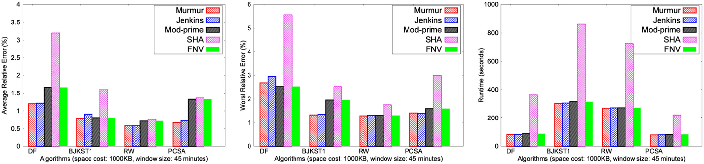
Figure 1. Comparison of hash functions for different algorithms using network trace.

3.1.1. Observation

MurmurHash has the most consistent accuracy, and its accuracy is better than all other hash functions that we considered. It also runs faster than the others. Jenkins and FNV are close to MurmurHash in terms of both accuracy and runtime. The total runtime of Modulo congruential hash is close to MurmurHash, but its accuracy is poor and inconsistent. SHA-1 performs the worst in terms of runtime, and the total runtime using SHA-1 is almost 2–3× slower than using MurmurHash, Modulo congruential hash and Jenkins. The accuracy of SHA-1 is consistent and better than Modulo congruential hash, but not as good as MurmurHash, Jenkins or FNV. Hence, we have chosen MurmurHash for the rest of our experiments.

3.2. Evaluation of Accuracy Boosting Method

The idea here is that the estimation accuracy can be improved by running multiple instances of an estimator, and combining the results in some manner. The use of accuracy boosting methods has been advocated in the past for distinct counting, including in Flajolet and Martin (1985), Gibbons and Tirthapura (2001), Bar-Yossef et al. (2002), and Kane et al. (2010). The goal of this set of experiments is to determine which accuracy boosting method serves best for an algorithm. We considered three methods, “median-of-many,” “split-and-add,” and “stochastic averaging,” which have been explained earlier in Section 2.2.

Any method such as the above certainly improves accuracy when compared with each individual estimator. However, when total memory of each algorithm is held fixed while increasing the number of instances, each instance gets proportionately smaller memory, resulting in lower accuracy for each individual instance. So it is not clear that accuracy boosting is useful to improve the overall accuracy of an algorithm given a fixed memory budget. Note that the past literature proves that accuracy boosting method such as the “median-of-many” method improves the overall accuracy of the algorithm provided the space allocated for the algorithm is also linearly increased.

From our experiments, we observed that, for the “median-of-many” method, the runtime increases linearly with the number of parallel instances, but it stays almost the same for split-and-add and stochastic averaging. The reason is that in the “median-of-many” method, the entire data stream is passed as input to, say, k different instances of algorithm resulting in linear increase in processing time for “median-of-many” method, contrary to the other two methods where data stream is divided into non-overlapping subsets which are in turn passed as input, each to an individual estimator of algorithm, hence resulting in no increase in runtime.

We implemented different accuracy boosting methods for each algorithm on every dataset. The findings for each dataset were similar. We found that RW performs best without accuracy boosting, i.e., when a single instance is used and the entire memory is given to that instance. Figure 2 shows the results of experiments performed using a space budget of 1,000 KB and window size 45 min on the network trace. Overall, the average relative error of RW without accuracy boosting method was better than with any accuracy boosting method. As the number of instances increase, the accuracy of the algorithm decreases due to the aforementioned reason. The total memory required by RW is O(log (1/δ)/ε²) words, where O(log (1/δ)) is the number of instances run for the algorithm. If the space budget is kept fixed, then the value of ε increases with the increase in the number of instances, resulting in a lower accuracy.

FIGURE 2

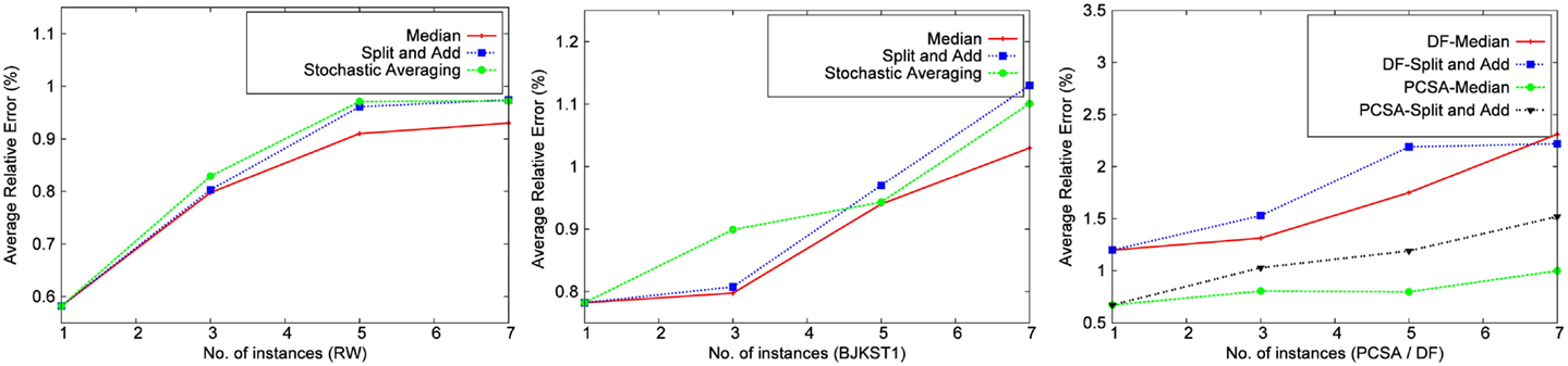
Figure 2. Comparison of accuracy boosting methods using network trace (space cost: 1,000 KB, window size: 45 min).

A similar result is observed with BJKST1 (Figure 2). The algorithm maintains the τ smallest hash values for each instance, and when multiple instances are used, the value of τ decreases proportionally to keep the overall memory constant. We found that the average relative error of BJKST1 was the smallest without accuracy boosting. While Bar-Yossef et al. (2002) suggested using the median-of-k, the study by Giroire (2009) and Zhang et al. (2010) suggested stochastic averaging as an improvement. Note that these did not focus on keeping the memory budget fixed while applying the accuracy boosting method to the algorithms. Per our observation, the average relative error is minimized by giving the entire memory to a single instance.

PCSA and DF combine many instances of a basic algorithm, which uses a bit vector of a fixed size, using stochastic averaging. We tried combining multiple instances of PCSA and DF using median-of-k method as well as split-and-add, but the error was worse when compared with using a single instance for both PCSA and DF (giving the entire memory to stochastic averaging). In Figure 2, using a single instance implies that only stochastic averaging is used over a fixed number of bit vectors determined from the space budget.

LC performs best when the entire space is given to a single instance. We tried using independent smaller bit vectors, followed by accuracy boosting, but this mostly led to invalid results. In case of median-of-k, the load factor of each smaller bit vector increased drastically, and the instances often failed to produce any reasonable estimates.

3.3. Evaluation of Algorithms

We implemented each algorithm using the best hash function (MurmurHash), and also the best accuracy boosting method specific to the algorithm. We ran experiments over all the 8 datasets for different space budget keeping the time-based sliding window fixed at 45 min. We also ran experiments over the 8 datasets for varying window size, keeping the space budget fixed at 1,000 KB. We have shown results for only 5 of the 8 datasets due to space constraint. We study the performance of algorithms for (1) different space budgets given a fixed window size (shown in Figures 3–7) and (2) different window sizes given a fixed space budget (shown in Figures 9 and 10). We find the median of 10 runs of each experiment to get the corresponding data point to obtain a consistent graph plot.

FIGURE 3

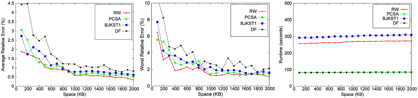
Figure 3. Dependence on space for network trace with a window size of 45 min.

FIGURE 4

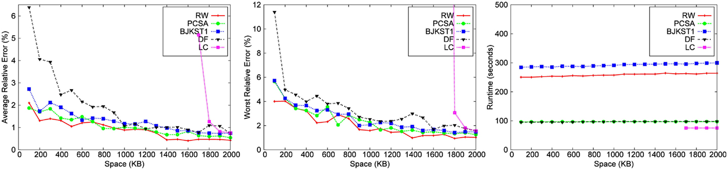
Figure 4. Dependence on space for Zipfian data with a window size of 45 min.

FIGURE 5

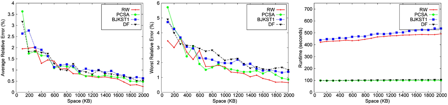
Figure 5. Dependence on space for Uniform Random dataset with a window size of 45 min.

FIGURE 6

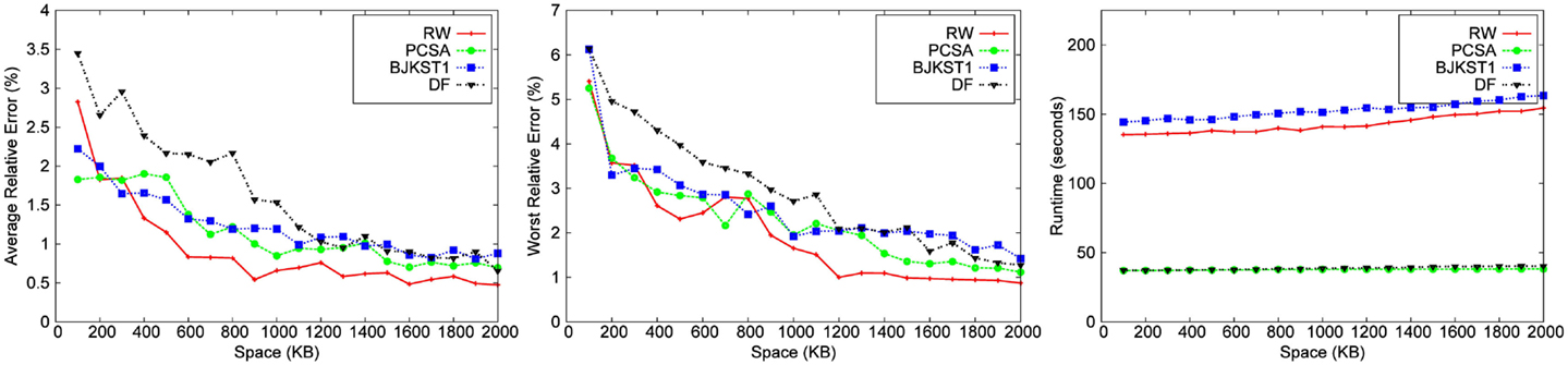
Figure 6. Dependence on space for Bigram dataset with a window size of 45 min.

FIGURE 7

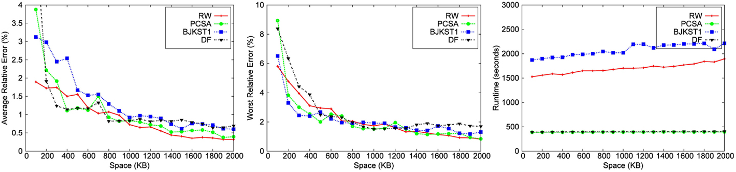
Figure 7. Dependence on space for Friendster graph data with a window size of 45 min.

3.3.1. Accuracy

We observe that for a fixed window size, the accuracy of RW and PCSA is the best for small-space budgets. As the allocated space is increased, the accuracy of RW becomes better than that of the other algorithms. We observe that as space increases, improvement in accuracy is the most significant in RW.

LC does not produce any result below a space threshold which depends on the number of distinct elements within the sliding window. Given a window size of 45 min, LC yields result for a minimum space of 1,700 KB for the Zipfian dataset. It does not produce a valid result for other datasets for a space budget as large as 2 MB. Among the other algorithms, we observe that PCSA and RW algorithm produces the most accurate result. As we increase the space budget, RW outperforms PCSA in terms of accuracy. According to the figures, DF algorithm is the least accurate algorithm.

In the study by Metwally et al. (2008), LC emerged as the most accurate algorithm for distinct counting for a given space budget, beating out PCSA and other alternatives. Our conclusions are different from those of Metwally et al. (2008), for the following reasons. First, note that their evaluation was for a different problem, that of distinct counting over an infinite window. The algorithms in Metwally et al. (2008) used a bit vector as a data structure to implement LC, which can accommodate a large number of distinct elements before the load factor gets too large, while we need to have a vector of timestamps to implement LC, which takes much more space (we used 32 bit timestamps). Furthermore, the number of distinct elements in the dataset used in Metwally et al. (2008) is ∼2 million, while the number of distinct elements in our datasets is much larger, leading to a higher load factor for the same memory allocated for LC. Since the accuracy of LC is very dependent on the number of distinct elements in the dataset, it is no longer the most accurate algorithm in our study, except for the case when the allocated memory is relatively large.

RW and PCSA are the two most accurate algorithms so we use Figure 8 to show the variation in the results obtained for RW and PCSA, respectively, over 10 different runs. These figures show the minimum, maximum, median, and first and third quartile values of average relative error obtained for RW and PCSA. From the figures, it is evident that these algorithms consistently perform well and that other than a few outliers, the variation in the average relative error is small (<1%). Due to a constraint in space, we have not added the graph for BJKST1, but the variation in BJKST1 is similar to RW and PCSA. We have also shown the variation in the results for DF algorithm over 10 runs in Figure 8. We observe that there is a large variation in the results for DF for small-space budget which gets better as the space allocated to the algorithm is increased.

FIGURE 8

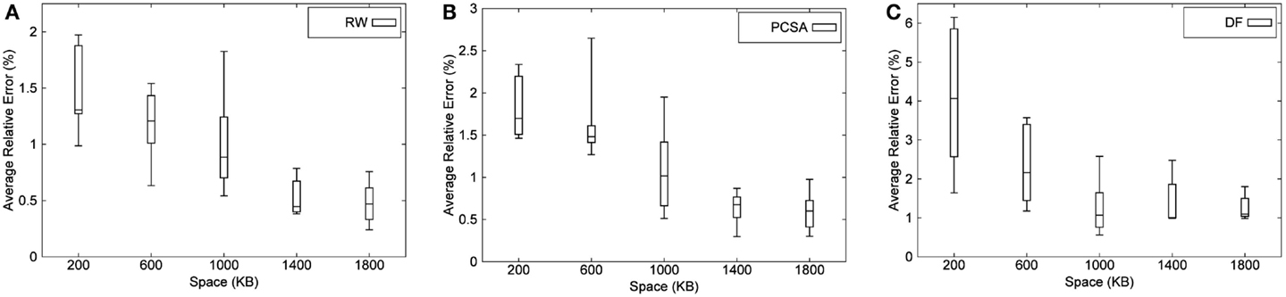
Figure 8. Distribution of average relative error of (A) RW, (B) PCSA, and (C) DF for Zipfian data (bottom and top of each box are 1st and 3rd quartiles, respectively, band within the box is the median, and uppermost and lowermost end of whiskers of each box are max and min, respectively).

We also performed an evaluation of the effect of the window size on the accuracy of each algorithm for a fixed space budget of 1000 KB (shown in Figures 9 and 10). We conclude from the figures that there is no clear correlation between the window size and the accuracy of algorithms. Also, the runtime of the algorithms do not seem to be affected when the window size is varied. The runtime of the algorithms do not vary with the window size because the total size of the dataset remains the same even when we vary the size of the window over which aggregation is performed. Though we have shown results for only the Bigrams dataset and the Friendster graph, we obtained the same result for the rest of the dataset.

FIGURE 9

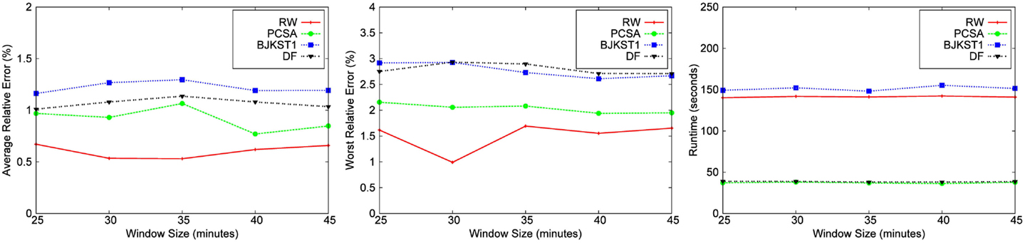
Figure 9. Dependence on window size for Bigram dataset for a fixed space budget of 1,000 KB.

FIGURE 10

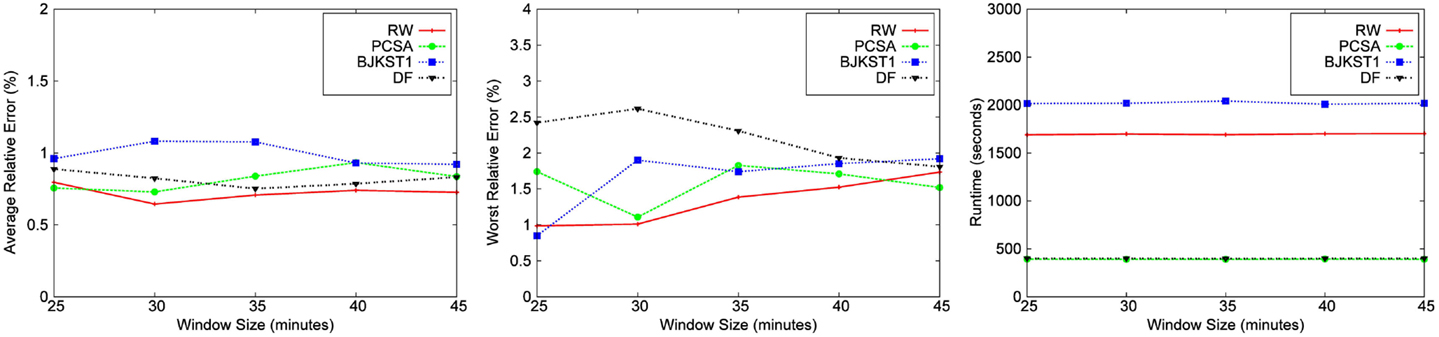
Figure 10. Dependence on window size for Friendster graph data for a fixed space budget of 1,000 KB.

3.3.2. Runtime

The running time of LC is the smallest followed by PCSA and DF. These algorithms are faster than RW (∼2–4 times) and BJKST1 (∼4–5 times), as shown in Figures 3–7. We observed that on increasing the space allotted to each algorithm, the runtime for each algorithm increases only slightly. While all the algorithms that we considered have O(1) (amortized) processing time per item, the processing times of these algorithms are different since PCSA, DF, and LC use very simple data structures (arrays) while RW and BJKST1 use a hash table as well as a list, which are relatively more expensive than an array.

We ran an experiment to compare the runtime performance of an array, an STL list, an STL unordered map (a hashmap with O(1) lookup time), and an STL map (an ordered map with O(log (n) lookup time, where n is the size of a dataset). We observed that the total time taken to insert 100,000 elements (elements inserted were valued 1–100,000) into an array is 1.3 ms whereas a simple insertion of elements in STL unordered map, STL map, and STL list is 14, 41, and 6.7 ms, respectively. Furthermore, we performed an additional experiment to measure the total time taken by STL unordered and ordered map to simultaneously insert and delete each input so that at no point in time, the map size is >1. The runtime for the unordered and ordered map for this experiment were 20 and 25 ms, respectively.

For RW and BJKST1 algorithms, there is an insertion in both map and list for each incoming element, whereas the deletion of elements from these data structures occurs at the end of every time unit. PCSA and DF algorithms require a simple insertion in an array for each incoming element. Considering that the number of insertions in array for PCSA and DF is the same as the number of insertions in both map and list for RW and BJKST1, in addition to the deletion of expired elements from RW and BJKST1 (note that PCSA and DF do not require to update the arrays for expired elements which leads to the significantly high query time for these algorithms), the difference in efficiency of list, map, and array is responsible for the difference in algorithm runtimes.

3.3.3. Query Frequency

The rate of queries (relative to the rate of updates) has an important bearing on the performance of an algorithm. We can think of two extremes here: one extreme is continuous monitoring, where there is a query after each update, and in the other extreme there is a query only at the end of observation. We use the term “query ratio” to mean the ratio between the number of updates and the number of queries for determining the number of distinct elements in the window.

While the performance of RW and BJKST1 is not affected much by the query ratio, LC, PCSA, and DF algorithms are significantly affected. In particular, answering a query using these algorithms requires a scan of the entire vector, which is very expensive. As described in Section 2.1, we also implemented a version of LC optimized for frequent queries, which we call LC2. We call the version that is not optimized for frequent queries as LC1. We could show the result pertaining to LC only for the Zipfian dataset. Other datasets need space much > 3 MB for producing a valid result for LC1 and LC2. We ran experiments over all the datasets using a space budget of 3 MB and a window size of 45 min. Smaller space allocation (<3 MB) did not work for LC2 even for the Zipfian dataset as the data structure used by LC2 requires large space. The X-axis represents the rate at which a query is posed. For instance, the x-value, 10,000, implies that a query is made every 10,000 updates. Figure 11 shows a significant increase in the runtime of LC1 as the rate of querying increases. LC2 performs consistently, without being affected by the rate of querying, similar to the other algorithms. However, this runtime of LC2 comes at the expense of accuracy, since additional space is taken up by the data structures for improving the query time. This also implies that LC2 would require much larger space for producing a valid result for a dataset.

FIGURE 11

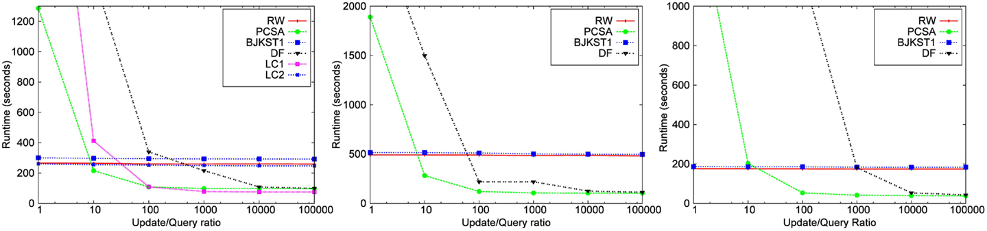
Figure 11. Dependence on rate of query for Zipfian data for a space cost 3,000 KB and a window size of 45 min.

Figure 11 also shows that the runtime of PCSA and DF is significantly large when query ratio is close to 1. However, the runtime of PCSA and DF, similar to LC1, reduces quickly with a decrease in query rate. The results from the Friendster graph and the network trace imply the same, but we have excluded it from the paper due to space constraint.

The runtime of LC1, PCSA, and DF algorithms increases drastically with query rate. This is because these algorithms require to perform a linear scan on the vector maintained by them so as to find the information that is required to compute the distinct count.

4. Discussion

We presented a detailed experimental evaluation of algorithms for distinct counting over a sliding window. We considered alternatives for different aspects of an implementation, including the basic algorithm, the hash function, the method for boosting accuracy, and the impact of query/update ratio. While there is no clear “best” method that works better than the rest under all situations, our experiments bring out a few combinations that work close to the best.

For a given space budget, if the average relative error is the most important criterion, then using a single instance of Randomized Wave algorithm with the Murmurhash function is close to the best in most situations. If execution time is the most important criterion, then for the scenario where the ratio of number of updates to the number of queries is low, PCSA using Murmurhash performs close to the fastest under most situations. However, if the ratio of updates to queries decreases, then the runtimes of PCSA and DF increase, and when this ratio is small (<100, in many cases), RW and BJKST1 perform better in terms of runtime. In such cases, RW is clearly the best option, both in terms of accuracy as well as runtime.

Overall, we observe that for a given space budget, random sampling-based schemes, such as RW, perform better than bitmap-based schemes, such as LC. This is because bitmap-based schemes, such as PCSA and LC, become more expensive space-wise when a timestamp is added to each bit in the vector, while a random sampling-based algorithm, such as RW, is not affected as much since it already stores the actual element identifiers in the sample, and adding a timestamp to the identifier does not increase the overhead by very much.

Funding

Supported in part by IBM PhD Fellowship.

Conflict of Interest Statement

The authors declare that the research was conducted in the absence of any commercial or financial relationships that could be construed as a potential conflict of interest.

Footnotes

1. ^https://sites.google.com/site/murmurhash/
2. ^http://www.burtleburtle.net/bob/hash/doobs.html
3. ^http://www.isthe.com/chongo/tech/comp/fnv/
4. ^https://tools.ietf.org/html/rfc3174
5. ^https://data.caida.org/datasets/oc48/oc48-original/
6. ^https://www.gutenberg.org/
7. ^http://snap.stanford.edu/data/index.html

References

Alon, N., Matias, Y., and Szegedy, M. (1996). “The space complexity of approximating the frequency moments,” in Proceedings of the Twenty-Eighth Annual ACM Symposium on Theory of Computing (STOC) (New York, NY: ACM), 20–29.

Google Scholar

Astrahan, M. M., Schkolnick, M., and Whang, K.-Y. (1987). Approximating the number of unique values of an attribute without sorting. Inf. Syst. 12, 11–15. doi: 10.1016/0306-4379(87)90014-7

CrossRef Full Text | Google Scholar

Bar-Yossef, Z., Jayram, T. S., Kumar, R., Sivakumar, D., and Trevisan, L. (2002). “Counting distinct elements in a data stream,” in Proceedings of the 6th International Workshop on Randomization and Approximation Techniques (RANDOM) (London: Springer-Verlag), 1–10.

Google Scholar

Braverman, V., and Ostrovsky, R. (2007). “Smooth histograms for sliding windows,” in Proceedings of the 48th Annual IEEE Symposium on Foundations of Computer Science (Washington, DC: IEEE Computer Society), 283–293.

Google Scholar

Busch, C., and Tirthapura, S. (2007). “A deterministic algorithm for summarizing asynchronous streams over a sliding window,” in Proceedings of the 24th Annual Conference on Theoretical Aspects of Computer Science (Aachen: Springer-Verlag), 465–476.

Google Scholar

Carter, L., and Wegman, M. N. (1979). Universal classes of hash functions. J. Comput. Syst. Sci. 18, 143–154. doi:10.1016/0022-0000(79)90044-8

CrossRef Full Text | Google Scholar

Charikar, M., Chaudhuri, S., Motwani, R., and Narasayya, V. (2000). “Towards estimation error guarantees for distinct values,” in Proceedings of the Nineteenth ACM SIGMOD-SIGACT-SIGART Symposium on Principles of Database Systems (PODS) (New York, NY: ACM), 268–279.

Google Scholar

Chen, A., and Cao, J. (2009). “Distinct counting with a self-learning bitmap,” in Proceedings of the 2009 IEEE International Conference on Data Engineering (ICDE) (Shanghai: IEEE Computer Society), 1171–1174.

Google Scholar

Datar, M., Gionis, A., Indyk, P., and Motwani, R. (2002). Maintaining stream statistics over sliding windows. SIAM J. Comput. 31, 1794–1813. doi:10.1137/S0097539701398363

CrossRef Full Text | Google Scholar

Durand, M., and Flajolet, P. (2003). “Loglog counting of large cardinalities (extended abstract),” in Proceedings of ESA 2003, 11th Annual European Symposium on Algorithms (Budapest: Springer), 605–617.

Google Scholar

Estan, C., Varghese, G., and Fisk, M. (2006). Bitmap algorithms for counting active flows on high-speed links. IEEE/ACM Trans. Netw. 14, 925–937. doi:10.1109/TNET.2006.882836

CrossRef Full Text | Google Scholar

Flajolet, P. (1990). On adaptive sampling. Computing 43, 391–400. doi:10.1007/BF02241657

CrossRef Full Text | Google Scholar

Flajolet, P., and Martin, G. N. (1985). Probabilistic counting algorithms for data base applications. J. Comput. Syst. Sci. 31, 182–209. doi:10.1016/0022-0000(85)90041-8

CrossRef Full Text | Google Scholar

Fraleigh, C., Moon, S., Diot, C., Lyles, B., and Tobagi, F. (2000). Architecture of a Passive Monitoring System for Backbone IP Networks. Sprint lab (TR00-ATL-101-801).

Google Scholar

Fusy, E., and Giroire, F. (2007). “Estimating the number of active flows in a data stream over a sliding window,” in Proceedings of the 9th Workshop on Algorithm Engineering and Experiments and the Fourth Workshop on Analytic Algorithmics and Combinatorics (Philadelphia, PA: Society for Industrial and Applied Mathematics), 223–231.

Google Scholar

Gelenbe, E., and Gardy, D. (1982). “The size of projections of relations satisfying a functional dependency,” in Proceedings of the 8th International Conference on Very Large Data Bases (San Francisco, CA: Morgan Kaufmann Publishers Inc.), 325–333.

Google Scholar

Gibbons, P. B. (2007). “Distinct-values estimation over data streams,” in In Data Stream Management: Processing High-Speed Data (Springer).

Google Scholar

Gibbons, P. B., and Tirthapura, S. (2001). “Estimating simple functions on the union of data streams,” in Proceedings of the Thirteenth Annual ACM Symposium on Parallel Algorithms and Architectures (SPAA) (New York, NY: ACM), 281–291.

Google Scholar

Gibbons, P. B., and Tirthapura, S. (2002). “Distributed streams algorithms for sliding windows,” in Proceedings of the Fourteenth Annual ACM Symposium on Parallel Algorithms and Architectures(SPAA) (New York, NY: ACM), 63–72.

Google Scholar

Gibbons, P. B., and Tirthapura, S. (2004). Distributed streams algorithms for sliding windows. Theory Comput. Syst. 37, 457–478. doi:10.1007/s00224-004-1156-4

CrossRef Full Text | Google Scholar

Giroire, F. (2009). Order statistics and estimating cardinalities of massive data sets. Discrete Appl. Math. 157, 406–427. doi:10.1016/j.dam.2008.06.020

CrossRef Full Text | Google Scholar

Golab, L., DeHaan, D., Demaine, E. D., Lopez-Ortiz, A., and Munro, J. I. (2003). “Identifying frequent items in sliding windows over on-line packet streams,” in Proceedings of the 3rd ACM SIGCOMM Conference on Internet Measurement (IMC) (New York, NY: ACM), 173–178.

Google Scholar

Haas, P. J., Naughton, J. F., Seshadri, S., and Stokes, L. (1995). “Sampling-based estimation of the number of distinct values of an attribute,” in Proceedings of the 21th International Conference on Very Large Data Bases (VLDB) (San Francisco, CA: Morgan Kaufmann Publishers Inc.), 311–322.

Google Scholar

Heule, S., Nunkesser, M., and Hall, A. (2013). “Hyperloglog in practice: algorithmic engineering of a state of the art cardinality estimation algorithm,” in Proceedings of the 16th International Conference on Extending Database Technology (EDBT) (New York, NY: ACM), 683–692.

Google Scholar

Kane, D. M., Nelson, J., and Woodruff, D. P. (2010). “An optimal algorithm for the distinct elements problem,” in Proceedings of the Twenty-Ninth ACM SIGMOD-SIGACT-SIGART Symposium on Principles of Database Systems (PODS) (New York, NY: ACM), 41–52.

Google Scholar

Lahiri, B., Chandrashekar, J., and Tirthapura, S. (2011). “Space-efficient tracking of persistent items in a massive data stream,” in Proceedings of the 5th ACM International Conference on Distributed Event-Based System (DEBS) (New York, NY: ACM), 255–266.

Google Scholar

Metwally, A., Agrawal, D., and Abbadi, A. E. (2008). “Why go logarithmic if we can go linear?: towards effective distinct counting of search traffic,” in 11th International Conference on Extending Database Technology (EDBT) (New York, NY: ACM), 618–629.

Google Scholar

Nasgaard, H., Gedik, B., Komor, M., and Mendell, M. (2009). “Ibm infosphere streams: event processing for a smarter planet,” in Proceedings of the 2009 Conference of the Center for Advanced Studies on Collaborative Research, CASCON ‘09 (Riverton, NJ: IBM Corp.), 311–313.

Google Scholar

Resvanis, M., and Chatzigiannakis, I. (2009). “Experimental evaluation of duplicate insensitive counting algorithms,” in Proceedings of the 2009 13th Panhellenic Conference on Informatics (Washington, DC: IEEE Computer Society), 60–64.

Google Scholar

Selinger, P. G., Astrahan, M. M., Chamberlin, D. D., Lorie, R. A., and Price, T. G. (1979). “Access path selection in a relational database management system,” in Proceedings of the 1979 ACM SIGMOD International Conference on Management of Data (New York, NY: ACM), 23–34.

Google Scholar

Singh, S. A., and Tirthapura, S. (2014). Monitoring persistent items in the union of distributed streams. J. Parallel Distrib. Comput. 74, 3115–3127. doi:10.1016/j.jpdc.2014.07.008

CrossRef Full Text | Google Scholar

Tirthapura, S., Xu, B., and Busch, C. (2006). “Sketching asynchronous streams over a sliding window,” in Proceedings of the Twenty-Fifth Annual ACM Symposium on Principles of Distributed Computing (New York, NY: ACM), 82–91.

Google Scholar

Tosun, A. S. (2007). “Space-efficient structures for detecting port scans,” in Proceedings of the 18th International Conference on Database and Expert Systems Applications (Berlin: Springer-Verlag), 120–129.

Google Scholar

Venkataraman, S., Song, D., Gibbons, P. B., and Blum, A. (2005). “New streaming algorithms for fast detection of superspreaders,” in Proceedings of Network and Distributed System Security Symposium, NDSS ‘05’ (San Diego, CA: Internet Society), 149–166.

Google Scholar

Whang, K.-Y., Vander-Zanden, B. T., and Taylor, H. M. (1990). A linear-time probabilistic counting algorithm for database applications. ACM Trans. Database Syst. 15, 208–229. doi:10.1145/78922.78925

CrossRef Full Text | Google Scholar

Whang, K.-Y., Wiederhold, G., and Sagalowicz, D. (1981). “Separability – an approach to physical data base design,” in Very Large Data Bases, Proceedings of the 7th International Conference (Cannes: VLDB Endowment), 320–332.

Google Scholar

Woodruff, D. (2004). “Optimal space lower bounds for all frequency moments,” in Proceedings of the Fifteenth Annual ACM-SIAM Symposium on Discrete Algorithms (Philadelphia, PA: Society for Industrial and Applied Mathematics), 167–175.

Google Scholar

Youssefi, K., and Wong, E. (1979). “Query processing in a relational database management system,” in Proceedings of the Fifth International Conference on Very Large Data Bases – Volume 5, VLDB ‘79 (Rio de Janeiro: VLDB Endowment), 409–417.

Google Scholar

Zaharia, M., Das, T., Li, H., Hunter, T., Shenker, S., and Stoica, I. (2013). “Discretized streams: fault-tolerant streaming computation at scale,” in Proceedings of the Twenty-Fourth ACM Symposium on Operating Systems Principles, SOSP ‘13 (New York, NY: ACM), 423–438.

Google Scholar

Zhang, W., Zhang, Y., Cheema, M. A., and Lin, X. (2010). “Counting distinct objects over sliding windows,” in Proceedings of the Twenty-First Australasian Conference on Database Technologies – Volume 104, ADC ‘10 (Darlinghurst: Australian Computer Society, Inc.), 75–84.

Google Scholar