View Sphere Partitioning via Flux Graphs Boosts Recognition from Sparse Views

1. Introduction

View-based object recognition has seen many recent advances with current state of the art systems achieving promising category-level recognition results on large databases of real images. An effective strategy here is to learn suitable models from images taken in a controlled fashion of several exemplars from a particular category (Fergus et al., 2007; Savarese and Fei-Fei, 2007; Wu et al., 2010). The hope here is that by learning from distinct views, one might be able to achieve recognition of nearby views efficiently. Such methods must be trained systematically on these distinct views and the typical strategy taken is to sample these views uniformly, as in the original principal component-based method of Murase and Nayar (1995). As our community attempts to grapple with the full complexity of object recognition from arbitrary views, we face the challenge that such methods may not easily generalize to views that have not been seen before, at least not without a prohibitive amount of training.

To gain further intuition about this problem, consider the sample silhouettes of a dog seen along two different trajectories in Figure 1. In the first trajectory, we move from a top rear view to a top front view (views 1–5) and in the second, we rotate around the dog showing side views (views 6–10). Qualitatively, views 6 through 10 are those from which the dog is most easily recognizable in that prominent parts (the head, limbs, and tail) remain visible. On the other hand, views in the first trajectory are more challenging to recognize because parts are foreshortened or occluded. This example points to the need for judicious view sphere sampling to achieve recognition from sparse views. Approaches that train on views sampled uniformly on the view sphere do not reflect the complex relationship between view stability and surface area on the view sphere.

FIGURE 1

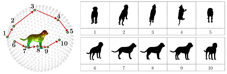
Figure 1. Silhouettes of a dog are shown for viewpoints along two trajectories on the view sphere: (1–5) and (6–10).

The problem of defining regions on the view sphere with qualitatively similar views of a 3D object has a long history in the computer vision community, dating back to Koenderink’s notion of transitions on the view sphere as one moves from one location to another, as signaled by the appearance or disappearance of singularities of the visual mapping (Koenderink and van Doorn, 1979). This lead to a tremendous interest in the computer vision community in computing aspect graphs designed to capture changes in appearance with viewpoint changes. A great deal of conceptual progress was made in the late 80s and early 90s with techniques developed for computing aspect graphs of polyhedra (Gigus et al., 1988) of curved surfaces described algebraically (Petitjean et al., 1992) along with considerations for the role of scale (Eggert et al., 1993). Whereas aspect graphs had intuitive appeal, they lost favor for a variety of reasons (Faugeras et al., 1992). These included the fragility of the concept itself for facilitating object recognition (e.g., not all singularities of the visual mapping are visually salient), and the difficulty of computing it for general 3D object classes. The object recognition community in computer vision has since shifted to appearance-based representations for category-level recognition from natural images of objects; see, for example, Ponce et al. (2006) and Dickinson (2009). Current approaches typically combine robust feature detection, the modeling of local geometric relations between derived “parts” and advanced statistical machine learning methods for classification (Lowe, 1999; Fei-Fei et al., 2006; Ferrari et al., 2006; Fergus et al., 2007; Wu et al., 2010). The underlying representations are viewpoint dependent, and thus, careful training is required for them to handle arbitrary views of 3D objects. As these methods advance from both computational efficiency and storage efficiency considerations, judicious sampling of the view sphere resurges as a problem of interest.

One way to approach this problem is to focus on the appearance of 2D silhouette shape as the viewpoint changes. Promising steps were taken in this direction by Cyr and Kimia (2004). In their approach, the views on the view sphere are treated as nodes of a graph, with the similarity between two views providing an edge weight. Their similarity measure uses both an edit distance between shock graphs and a distance based on curve matching. Each node on the view sphere is initially a cluster (region), and clusters get merged when they are geographical neighbors and the average pairwise similarities between their centroids are below a certain threshold. This process is iterated until it converges. Once the regions have been obtained, at matching time, a query view is matched against the centroid (characteristic view) of each region for a particular model. Those regions whose centroids are distant from the query are discarded. The model is then matched exhaustively against all the views in each surviving region.

Motivated by the success of medial representations for computing part-based representations of silhouettes for matching (Sebastian et al., 2004; Bai and Latecki, 2008; Siddiqi and Pizer, 2008) and the promise of silhouette-based similarity for 3D recognition in Cyr and Kimia (2004), we consider the problem of recognition from sparse views using skeletal graphs. The specific question we look at is that of generating view sphere partitions from which to efficiently (and not necessarily exhaustively) sample model views when faced with a new query. As such our goal is complementary to that of Cyr and Kimia (2004), but our methods are different. Specifically, we employ an average outward flux-based skeleton (Dimitrov et al., 2003) together with a novel measure for simplification which leads to a directed flux graph. In our work, we employ a hierarchical clustering algorithm to obtain a view sphere partition where views in each partition are similar. Unlike the region-growing approach of Cyr and Kimia (2004), our partitions are based on a spectral decomposition strategy, which lead to partitions whose nodes are not necessarily geographical neighbors. More importantly, the context of our experiments is different and somewhat complementary to that of Cyr and Kimia (2004). Specifically, we evaluate the benefit of selecting model views from the partitions when only a sparse number of model view queries are allowed, whereas in Cyr and Kimia (2004), the matching experiments use all the model views in each surviving cluster. Our main contribution is to show that hierarchical view sphere partitioning boosts 3D object recognition performance in the scenario of matching against a sparse number of model views. Our experiments also demonstrate the importance of selecting centroids of the clusters during matching time for the four shape matching algorithms we have evaluated: shape context-based matching, inner distance-based matching, flux graph matching, and shock graph matching.

This article is organized as follows. We discuss flux graphs for 2D shape representation in Section 2. We then develop the view sphere partitioning strategy in Section 3, where a clustering algorithm is employed on a graph whose nodes are views and whose edge weights are pairwise similarities between flux graphs. This leads to partitions within which the model silhouettes are qualitatively similar. We demonstrate the utility of these partitions for selecting model views in Section 4 by comparing this to the alternatives of random or uniform sampling. We conclude with a discussion in Section 5.

2. Flux Graphs

DEFINITION 1. Assume an n-dimensional object denoted by Ω with its boundary given by ∂Ω ∈ ℝⁿ. A closed disk D ∈ ℝⁿ is a maximal inscribed disk in Ω if D ⊆ Ω but for any disk D′ such that D ⊂ D′, the relationship D′ ⊆ Ω does not hold.

DEFINITION 2. The Blum medial locus or skeleton, denoted by Sk(Ω), is the locus of centers of all maximal inscribed disks in ∂Ω.

Topologically, Sk(Ω) consists of a set of branches that join to each other at junction points to form the complete skeleton. A skeletal branch denoted by χ is a set of contiguous regular points from the skeleton that lie between a pair of junction points, a pair of end points or an end point and a junction point. As shown by Dimitrov et al. (2003), these three classes of points can be analyzed by considering the behavior of the average outward flux (AOF) of the gradient of the Euclidean distance function to the boundary of a 2D object, given by $\frac{{\int }_{\mathrm{\partial R}}<\dot{\mathbf{\text{q}}},\mathbf{\text{N}}>\mathit{ds}}{{\int }_{\mathrm{\partial R}}\mathit{ds}}$, when shrunk to a circular neighborhood, where $\dot{q}=\nabla D$ (Dimitrov et al., 2003), with D the Euclidean distance function to the object’s boundary. In particular:

1. p is a regular point if the maximal inscribed disk at p touches the boundary at two corresponding boundary points such that |Π_Ω(p)| = 2 (the projection Π_Ω(p) is the set of closest points on the boundary ∂Ω to p, i.e., Π_Ω(p) ≜ {q ∈ ∂Ω:||p − q|| = min{||p − q||∀q ∈ ∂Ω}}. Let F _ε(p) represent the total outward flux through a shrinking circular region around the neighborhood of P with radius ε. The computed AOF at a regular point p is then given by ${\lim }_{\mathrm{\epsilon }\to 0}\frac{{\mathbf{\text{F}}}_{\mathrm{\epsilon }}\left(\mathbf{\text{p}}\right)}{2\pi \epsilon }=-\frac{2}{\mathrm{\pi }}\sin \mathrm{\theta }$.

2. p is an end point if there exists δ (0 < δ < r) such that for any ε (0 < ε < δ) the circle centered at p with radius ε intersects Sk(Ω) just at a single point (r is the radius of the maximal inscribed disk at p). The computed AOF at an end point p is given by ${\lim }_{\mathrm{\epsilon }\to 0}\frac{{\mathbf{\text{F}}}_{\mathrm{\epsilon }}\left(P\right)}{2\pi \mathrm{\epsilon }}=-\frac{1}{\mathrm{\pi }}\left(\sin {\mathrm{\theta }}_{\text{P}}-{\mathrm{\theta }}_{\text{P}}\right)$.

3. p is a junction point if Π_Ω (p) has three or more corresponding closest boundary points. Generically, a junction point has degree 3. All other junction points are unstable. The computed AOF at a junction point p is given by ${\lim }_{\mathrm{\epsilon }\to 0}\frac{{\mathbf{\text{F}}}_{\mathrm{\epsilon }}\left(P\right)}{2\pi \mathrm{\epsilon }}=-\frac{1}{\mathrm{\pi }}{\sum }_{\text{i}=1}^{\text{n}}\sin {\mathrm{\theta }}_i$.

We adopt the AOF approach of Dimitrov et al. (2003) to compute the flux-based skeleton. We then consider the degree to which the area reconstructed by the maximal disk associated with a skeletal point is unique. Specifically, for each skeletal point, we compute the fraction of area of its maximal disk that does not overlap with the disk of a skeletal point on any other branch. This relative area contribution measure is novel to the literature and is particularly simple to compute while being effective. The measure decreases monotonically as one approaches a junction point, as illustrated by the three sample calculations in Figure 2 (left). Numerous other salience measures for medial loci have been proposed (Siddiqi and Pizer, 2008) but most combine a notion of boundary-to-axis ratio, which can be delicate to compute, with the object angle, and require choices of thresholds and parameters to be tuned. The monotonic decrease in the relative area measure as one approaches a junction point suggests a more robust simplification procedure, which is to move in the direction away from a junction point and retain only those skeletal points with relative area measure above a threshold. This process is illustrated for the dog shape in Figure 2 (right). The threshold can be chosen adaptively to ensure that a desired percentage of the original shape’s area is captured, as illustrated in Figure 3 (left). For all the experiments and examples in this article, we require at least 95% area coverage. The parts reconstructed by each black skeletal segment are shown in distinct colors, with skeletal segments which have been removed by the simplification process shown in light pink.

FIGURE 2

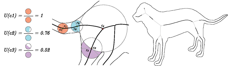
Figure 2. Left: for the three skeletal points, c1, c2, and c3, we calculate the fractional area of the maximal inscribed disk that does not overlap with that of a skeletal point on any other branch. This relative area measure decreases monotonically as one approaches a junction point. Right: the skeletal points with fractional maximal disk area above a threshold are shown in black, with other flux-based skeletal points shown in gray. The threshold is chosen so that the black skeletal segments reconstruct at least 95% of the shape’s area [see Figure 3 (left)].

FIGURE 3

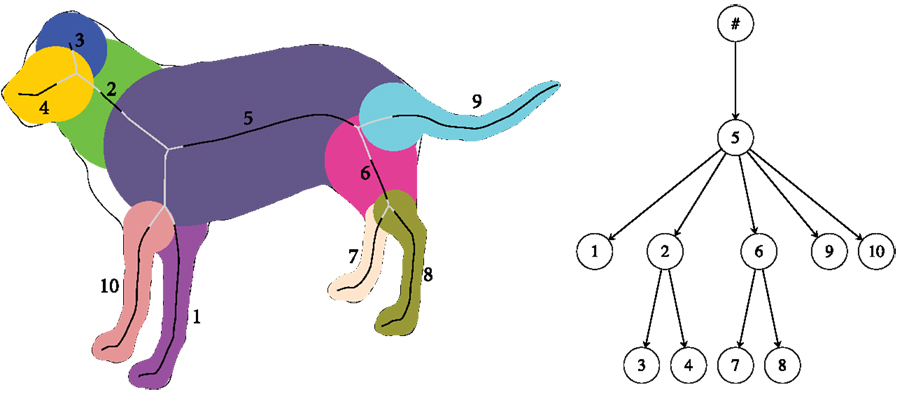
Figure 3. Left: the nodes corresponding to the retained skeletal segments (black) are shown in different colors, each representing a union of medial disks. Right: the corresponding flux graph. The dummy node # carries no geometrical information but serves as a parent to all the top level nodes.

The monotonicity property ensures that for each original skeletal branch, at most one skeletal segment is retained. We can therefore associate each retained skeletal segment with the node of a graph. Then, using the topology of the original skeleton, for any set of adjacent nodes, edges are placed in the direction from the node having the largest average maximal inscribed disk radius to the others. The resulting directed acyclic graph represents a hierarchy of parts, as illustrated for the dog shape in Figure 3 (right), which we dub the flux graph. As it turns out, this simplification procedure, based on relative area alone, is more robust than the strategy first proposed in Rezanejad and Siddiqi (2013).

2.1. Flux Graph Matching

In the present article, we use the established method for matching directed acyclic graphs (DAGs) in Siddiqi et al. (1999) for flux graph matching. Given two flux graphs a bipartite graph is constructed between their nodes in a hierarchical manner. Each edge of the bipartite graph is weighted based on the structural similarity between the nodes. This weight is based on the normalized difference between the topological signature vectors (TSVs) introduced in (Siddiqi et al., 1999). A maximum weighted bipartite matching is then carried out such that the sum of the values of the edges is maximized. In a DAG representation, the TSV is defined as the vector of eigenvalue-sums derived from the corresponding adjacency matrix for the sub-DAG of the considered node. The matching algorithm used is a greedy algorithm by Macrini et al. (2008), which has the benefit of finding a largest maximal matching in polynomial time. The similarity is computed by matching a query with a model node and then normalizing that by the number of matched nodes according to the cardinality of the model graph.

The above structural similarity measure (Γ) is combined with a notion of the geometric similarity (Δ) between the parts corresponding to two nodes, where for the latter we use the elastic matching approach in Macrini et al. (2008). Here, line segments are fit through the skeletal points of a given node and then, for a given query and a given model, the algorithm tries to fit the query to the model by allowing line segments of the model to shrink or grow to include the query data points. The data points themselves encapsulate both positions along a skeletal branch and the radius of the maximal inscribed disk. The main assumption here is that the pattern of velocities and acceleration is invariant to small changes in viewpoint, where velocity and acceleration are defined as first and second derivatives of the radius along the medial axis.

Putting these measures of similarity together, a DAG matcher receives two DAGs G₁ and G₂ as input and computes a value S(G₁, G₂) representing the similarity between them, as well as a list of corresponding nodes. Both Γ and Δ are in the interval [0 1] and S(G₁, G₂) is given by a weighted combination: ωΓ(G₁, G₂) + (1 − ω)Δ(G₁, G₂). Here, ω is a tuning weight in the interval [0 1].

3. View Sphere Partitioning

We use the flux graph to represent the silhouette seen from each view on the view sphere of an object. We then create a dense view sphere graph by associating each view with a node and placing an edge between each pair of nodes. To each edge, we associate a weight based on the similarity between the views using the DAG matcher described above. The problem of view sphere clustering can now be treated as a clustering problem on the view sphere graph. Our goal is to find clusters of view sphere points with high within cluster similarity. Such clusters should, in principle, correspond to regions of the view sphere within which the silhouette shapes are similar. To this end, we employ a clustering algorithm but in a hierarchical fashion. Intuitively, the idea is to recursively partition clusters until a particular derived cluster has a high enough within cluster similarity and is then treated as a leaf node of a view sphere graph. The final set of clusters then correspond to the set of leaf nodes.

Within cluster, similarity is of course maximized when the clusters are very small, so we impose a minimum cluster size for partitioning. Given a view sphere ν, we find a suitable number of clusters for decomposition (Algorithm 2) and then the hierarchical clustering algorithm is applied recursively (Algorithm 1). A stopping condition (Algorithm Algorithm 3) is imposed whereby a cluster is no longer divided if it is small (in practice, its size is already <10% of the view sphere) or if the average of the pairwise similarities within that cluster is above a threshold.

ALGORITHM 1

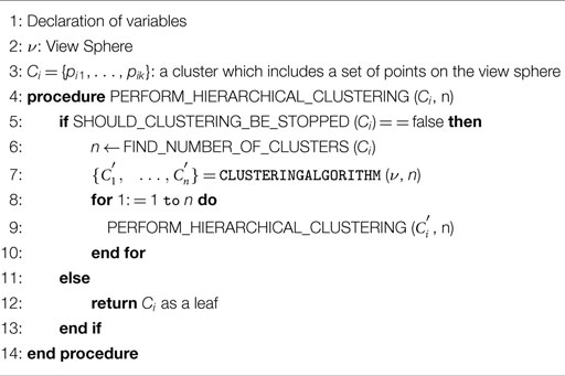
Algorithm 1. Hierarchical view sphere clustering.

ALGORITHM 2

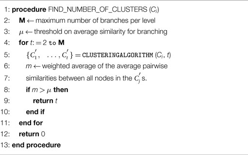
Algorithm 2. Find the number of clusters for decomposition.

ALGORITHM 3

Algorithm 3. Determine whether a cluster is a leaf node.

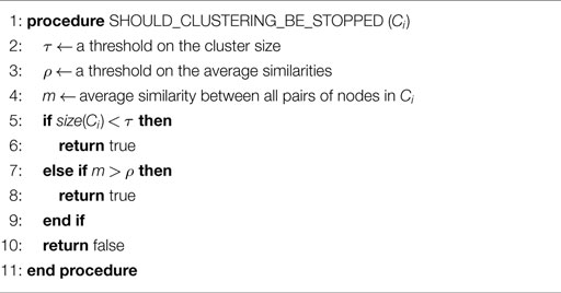
Using 128 equi-spaced viewing directions, Figure 4 (left) illustrates the view sphere clusters obtained for the dog using the method above. Regions of the view sphere belonging to the same cluster are shown in the same color, in separate panels (1–6). For this example, there is an inherent symmetry to the clusters, such that each is composed of two diametrically opposed regions on the view sphere. To give a sense of the manner in which the views within a particular cluster are similar with regard to part structure and part shape, Figure 4 (right) depicts sample silhouettes for trajectories taken within each cluster. Cluster 1 contains views from above or below such that the body is elongated and the tail is visible but the limbs are occluded. In contrast, clusters 3 and 4 depict side views in which the limbs are visible and are extended.

FIGURE 4

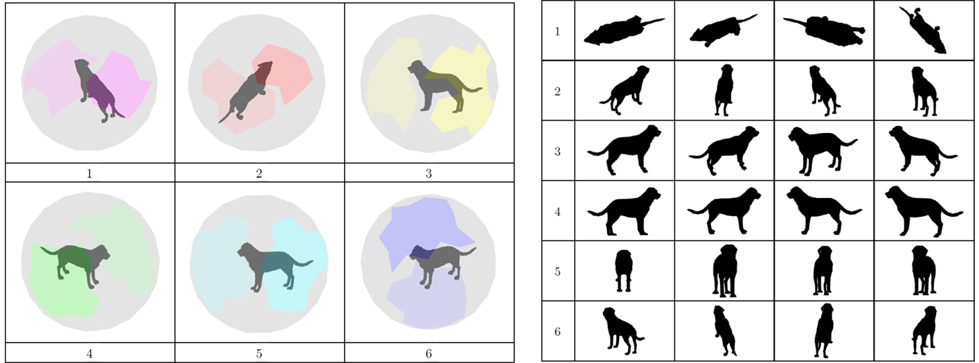
Figure 4. Left: views of the dog on the view sphere belonging to the same cluster are shown as colored regions with distinct colors in panels (1–6). Right: silhouettes are shown for views sampled from each of the clusters on the left. See the text for a discussion.

4. Experiments

We evaluate the efficacy of using our view sphere partitions for recognition from sparse views. In our recognition experiments, we consider a query view and compare matching it with model views chosen from the view sphere clusters proportional to their size versus matching it against model views chosen randomly from a uniform distribution of views on the view sphere. We have also conducted experiments where the model views were chosen to spread across the view sphere evenly, by using a particle repulsion method such that the distance between all pairs of neighboring closest model views was approximately the same. However, we found that in all cases, random sampling from a uniform distribution out performs this particle repulsion strategy. This is likely because spreading the views across the view sphere leads to a higher probability of selecting model views that are ambiguous in that they are less representative of a particular object. We compare four different silhouette matching approaches: flux graph matching, shock graph matching, shape context-based matching, and inner distance-based matching. The skeletal graph-based matching experiments are carried out using Macrini’s publicly available directed acyclic graph (DAG) matching package: http://www.cs.toronto.edu/~dmac/download.html, which contains an implementation of the approach in Siddiqi et al. (1999). For shape context-based matching (Belongie and Malik, 2000), we use the original implementation by Belongie et al., available at https://www.eecs.berkeley.edu/Research/Projects/CS/vision/shape/sc_digits.html, and for inner distance-based matching (Ling and Jacobs, 2007), we used Ling and Jacobs’ implementation, available at http://www.dabi. temple.edu/∼hbling/code_data.htm.

Both shape context-based matching and inner distance-based matching rely on finding correspondences between sample points from the boundaries of the two silhouettes. In the former, the shape context descriptor is based on a histogram of the contour points present in a local polar neighborhood of each sample point, considering both Euclidean distance and relative position. Two silhouettes are then matched using the Hungarian algorithm for finding the lowest cost matching between the two sets of histograms. This approach is extended in Ling and Jacobs (2007) by replacing the Euclidean distance by a notion of inner distance. The inner distance is defined as the length of the shortest path within the silhouette between two boundary points, and it provides some robustness to part articulation. A silhouette is represented in the same way as when using the shape context descriptor but with the difference that the bins in the histogram are constructed using inner distance in place of Euclidean distance. The tangential direction at the starting point of the shortest path between two points is treated as the relative orientation between them, and is called the inner angle. Two silhouettes are matched by finding the lowest cost matching between the two histograms, but allowing for boundary sample points to be skipped but with an associated penalty.

4.1. Recognition Performance

4.1.1. Exemplar Level Recognition

We begin with the exemplar level Toronto database of 19 models (Figure 5 left) because of the available published experimental results on skeletal graph-based recognition in Macrini et al. (2008) as views are successively removed for these objects. In that work, Macrini et al. remove up to 75% of the views on the view sphere for a subset of 13 object models from this database, with 128 views of each. They report a graceful degradation in performance with occlusion, achieving 87% correct recognition with the shock graph as the representation. We carry out similar experiments evaluating flux graph matching, shock graph matching, shape context-based matching, and inner distance-based matching. Our goal is to demonstrate that in a sparse model view selection scenario, sampling these views from our view sphere partitions can boost recognition performance in all cases.

FIGURE 5

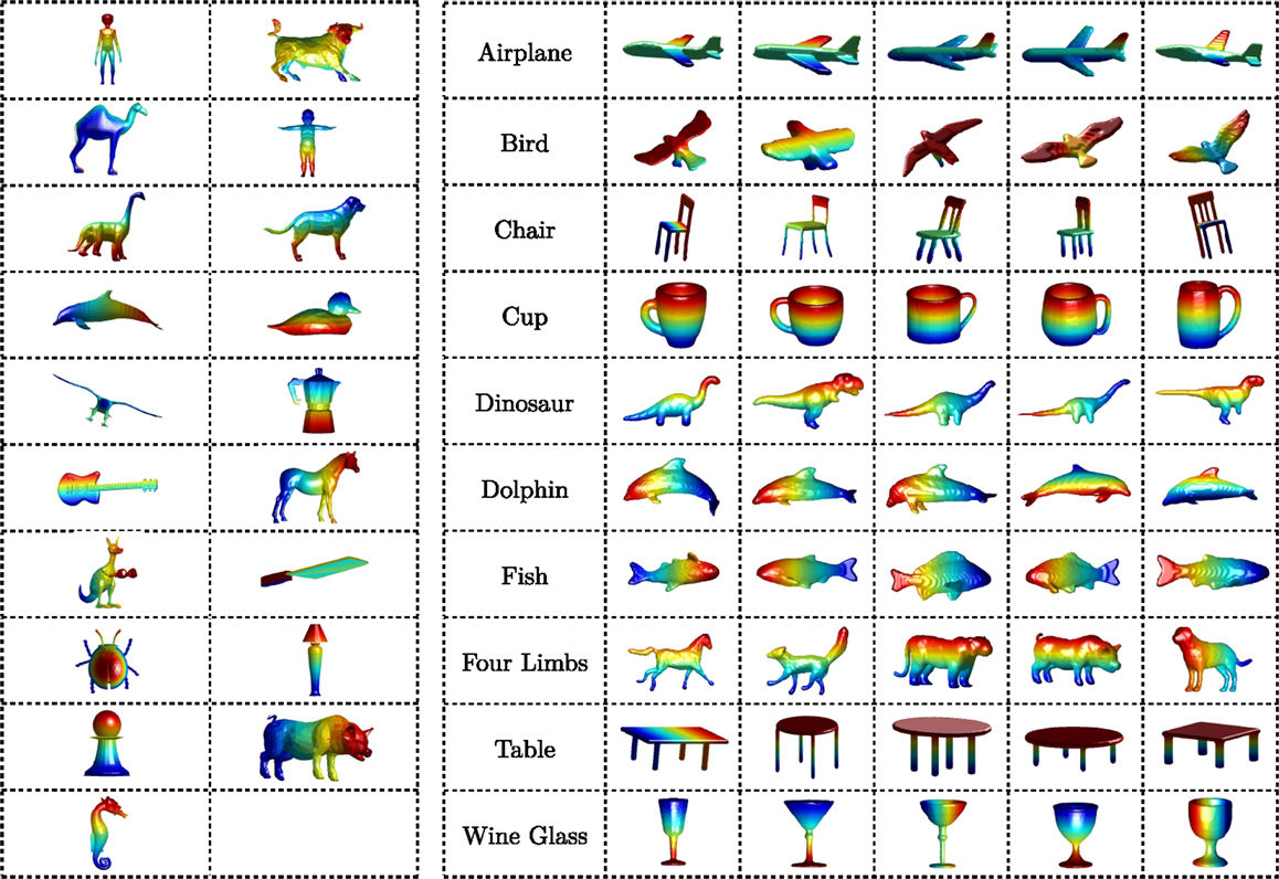
Figure 5. Left: the 19 object models in the Toronto database which we use for our experiments in exemplar level recognition. Right: a selection of the 150 models from the McGill 3D Shape Benchmark which we use for our experiments in category-level recognition. In total, we have 10 object classes with approximately 15 models in each.

The 19 Toronto database models are scaled to fit in a view sphere having radius 1. On this sphere, we sample 128 views using a particle repulsion based approach for node placement (Saff and Kuijlaars, 1997). For each object, we construct a view sphere tree with the following choices of parameters. First, the minimum cluster size for partitioning is chosen to be 12 view points. Thus, any cluster smaller than this size is not further partitioned. Second, the average within cluster pairwise similarity threshold, where the pairwise similarities are obtained using the DAG matcher, is set to 0.65 (on a scale from 0 to 1). Thus, any cluster with an average pairwise similarity higher than this threshold is not further subdivided. These view sphere partitions are computed offline. In our experiments, we have evaluated both the Normalized Cuts clustering algorithm of Shi and Malik (2000) using the package at http://www.cis.upenn.edu/~jshi/software/ and the K-medoids algorithm based on the implementation at http://www.mathworks.com/help/stats/kmedoids.html for clustering. Both lead to very similar recognition performance for all four shape matching methods; so both here and for category-level recognition, we present results based on the Normalized Cuts algorithm.

At recognition time, we match a query view against a sparse set of 8 sample views for each model, representing about a 94% reduction in view sphere nodes. These samples are chosen proportional to cluster size, i.e., the number of samples taken from each cluster depends on the area of that cluster relative to the entire view sphere. The first sample from a cluster is chosen to be its centroid, while the rest are picked randomly. The centroid of a cluster is defined as that view whose average pairwise similarity with all other views in the cluster is maximum. In what follows, we refer to this geographical area-weighted view selection strategy as partition sampling.

In the first set of experiments, we match all 19 × 128 views from the database to the 19 × 8 sample views, taking care not to ever match a silhouette with itself. We find the best match and define it to be correct if it corresponds to a view of the same object. We then repeat this experiment and define the best match as the one with the majority vote among n closest samples, with n varying from 1 to 30. In the second set of experiments, we match all 19 × 128 views from the database to 8 views of each of the 19 objects that are now chosen at random. The results of random sampling (dashed lines) versus partition sampling (solid lines) are reported in Figure 6 for shape context matching (green), inner distance matching (purple), flux graph matching (blue), and shock graph matching (red). It is striking that partition sampling consistently boosts recognition performance over random sampling, i.e., the solid lines are above the dashed counterparts. There is also strong evidence that in a scenario of recognition from sparse model views, skeletal (flux graph or shock graph) matching out performances shape context-based matching and inner distance-based matching. The results for shock graph matching are slightly better than those for flux graph matching because the elastic matching approach to geometric similarity between nodes in Macrini’s DAG matcher is optimized for shock graphs.

FIGURE 6

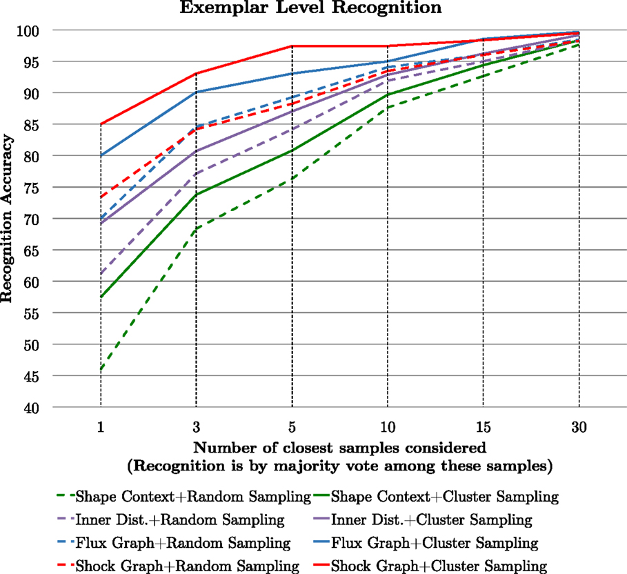
Figure 6. We compare view sphere partition sampling (solid lines) of model views against random sampling (dashed lines) of model views for four shape matching methods applied to an exemplar level recognition task. See the text for a discussion.

4.1.2. Category-Level Recognition

We now carry out a more ambitious set of recognition experiments at the category level using a selection of 150 models from the McGill 3D Shape Benchmark. The process is exactly the same as that used for exemplar level recognition above, except that we now have 150 × 128 query views to match. A recognition trial is assumed to be correct when the best match is with a model within the same category. This task is inherently more challenging than the exemplar level recognition task, due to the similarity in shape between some of the object categories (e.g., four limbed and dinosaur, as well as fish and dolphin) and also due to the significant variation in shape within an object class (e.g., four limbed). The results of random sampling (dashed lines) versus partition sampling (solid lines) are reported in Figure 7 for shape context matching (green), inner distance matching (purple), flux graph matching (blue), and shock graph matching (red). Once again, it is striking that partition sampling boosts recognition performance over random sampling. Averaging over all the 150 × 128 queries, the improvement is from 59.60 to 71.70%, using shape context matching, from 67.04 to 77.52% using inner distance matching, from 85.52 to 89.18%, using flux graph matching and from 86.56 to 91.20%, using shock graph matching. The relative performance of the four matching methods is similar to that for exemplar level recognition, except that flux graph matching is now almost on par with shock graph matching.

FIGURE 7

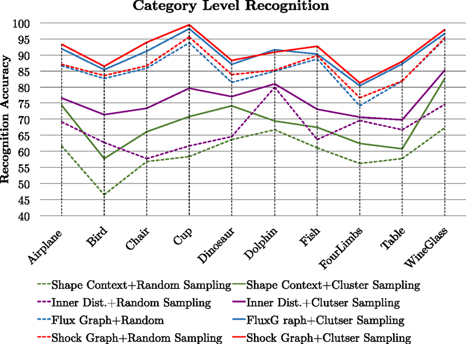
Figure 7. We compare view sphere partition sampling of model views against random sampling of model views for four shape matching methods applied to a category-level recognition task. See the text for a discussion.

4.1.3. Exploring Different Sampling Strategies

We now consider alternate model view sampling strategies for both the exemplar and category level recognition experiments, under the same sparse view scenario as before. We compare four different approaches. In the first (VS1), the model views are selected randomly from a uniform distribution on the view sphere. In the second (VS2), the model views are selected randomly from our view sphere partitions, but with the number of views from each partition being proportional to its size. The third approach (VS3) is similar to the second, with the exception that the first view from a partition is chosen to be its centroid. The fourth approach (VS4) is similar to the third except that now additional views from a partition, when required, are now selected in decreasing order of average pairwise similarity to the other views in that partition. As such the view sphere sampling strategies VS1 and VS3 are those used in Sections 4.1.1 and 4.1.2, but VS2 and VS4 are new. The results, averaged over all the objects, are presented in Figure 8 for the four shape matching strategies at the exemplar level (left) and the category level (right). These results demonstrate the importance of choosing the centroid as the first sample view. Notably, as we move from random sampling (VS1) to random sampling from partitions but with the number of views proportional to partition size (VS2) the improvement is slight. However, when moving to VS3, where the first view from a partition is its centroid, we see a boost in performance of up to 10% in some cases. The additional benefit of selecting subsequent views from a partition in decreasing order of average pairwise similarity to the other views in that partition (VS4) is only slight. This is likely because in our sparse model view scenario not many partitions end up having more than one model view.

FIGURE 8

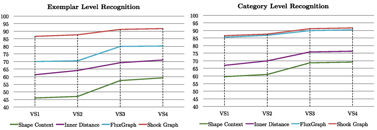
Figure 8. We compare recognition performance under different sampling strategies, with the results averaged over all the objects in the database at the exemplar level (left) and the category level (right). See the text for a discussion.

4.2. Flux Graphs Versus Shock Graphs

Whereas shock graphs outperform flux graphs for exemplar level recognition, in part because of the optimization of the matcher for them, the narrowing of this gap for category-level recognition combined with the simplicity of flux graphs offers certain advantages. Using the 19 models in the Toronto database, but now with 1000 views of each, and using a subset of 110 objects of the 150 used for category-level recognition from the McGill Shape Benchmark, but now with 1000 views of each, we compare shock graphs using the publicly available code at http://www.cs.toronto.edu/~dmac/download.html with flux graphs using a number of complexity measures: the average number of nodes, the average number of edges, the average depth, the average number of skeletal points, and the average TSV (topological signature vector) component values. The results, presented as $\frac{\text{fluxgraph}}{\text{shockgraph}}$ ratios in Figure 9, show similar trends for both databases: flux graphs have 40% or fewer edges and nodes than shock graphs and 30% fewer skeletal points.

FIGURE 9

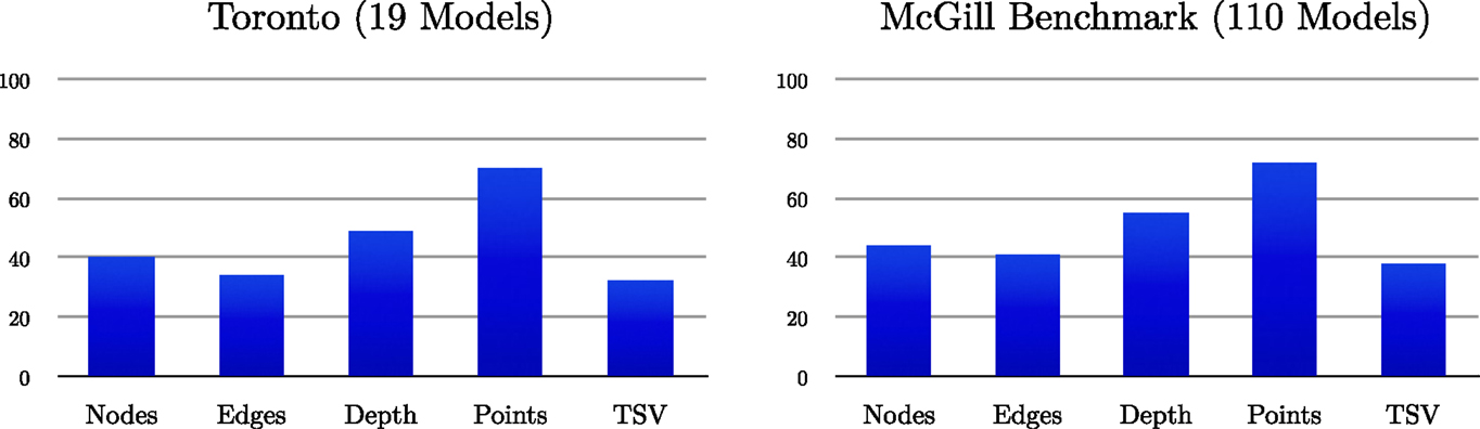
Figure 9. We plot the ratio of several complexity measures between flux graphs and shock graphs, as percentages, for the Toronto database of 19 models with 1000 views of each (19,000 silhouettes in total) and for 110 models from the McGill 3D Shape Benchmark with 1000 views of each (110,000 silhouettes in total). See the text for a discussion.

4.3. Running Time Complexity

We now consider how the matching methods evaluated in this paper stand against one another in terms of running time complexity. The task of recognition is divided into two parts: representation creation and matching a query representation against another one. For both flux graphs and shock graphs, a skeletal graph is constructed for each view and is stored in memory. For shape context and inner distance, we extended the original implementations to avoid repetition during the matching phase. In particular, for each silhouette, we compute the representation histograms first and store these in memory. Since each query silhouette is matched against a very large database of views, this preliminary step of precomputing and storing the histograms speeds up the matching phase considerably.

To measure the running time of these algorithms, we considered the following set up: 3 different views were selected randomly from each of the 150 models from the McGill 3D Shape Benchmark. One of these views was added to the query set and the other two to the model set. Thus, we had a total of 450 silhouettes. For each of the four methods, we then measured the time to (a) create the representations and (b) match the query against the model views. During the matching phase, we matched the 150 queries views to each of the 300 model views. The total running time, in seconds, is listed in Figure 10. All the experiments were performed on a PC with a 2.4-GHz Intel(R) Core(TM) i7-4700MQ CPU, 8 GB RAM, an NVIDIA GeForce GT 750M graphics card, and a 250-GB SSD disk. For these measurements, we used Windows 8.1 Pro. To generate a fair comparison, the input silhouettes were normalized to have the same resolution and initial number of boundary points.

FIGURE 10

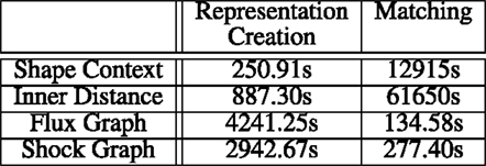
Figure 10. Running time complexity for the four shape matching algorithms. See the text for a discussion.

These results show that flux graphs and shock graphs are slower to compute than representations based on shape context or inner distance. However, flux graph and shock graph matching, using Macrini’s DAG matcher, are significantly faster than inner distance-based matching or shape context-based matching. This may in part due to the actual complexity of the associated algorithms in terms of number of operations but also in part due to the fact that the DAG matcher package is implemented in C/C++, while the others are designed to be user friendly and use non-optimized code, e.g., based on Matlab.

5. Discussion

In the present article, we have demonstrated the promise of view sphere partitioning for 3D recognition from sparse views, by the hierarchical application of a clustering algorithm on pairwise similarities computed between flux graphs. Our experiments at the exemplar level on the Toronto model database (19 × 128 silhouettes) and at the category level on a selection of objects from the McGill 3D Shape Benchmark (150 × 128 silhouettes) demonstrate the consistent improvement possible by partition sampling of model views during the recognition phase, using the generated view sphere partitions. This improvement applies to each of the four shape matching algorithms we have evaluated: shape context-based matching, inner distance-based matching, flux graph matching, and shock graph matching.

Our work suggests a number of fruitful directions for further research, having to do with the use of precomputed view sphere partitions in online recognition scenarios. Clearly, there is rich information contained in the silhouette of an object by which to facilitate 3D recognition and with 3D point cloud data of real 3D objects now within reach of computer vision researchers via Kinect type sensors, offline computation of view sphere partitions is becoming feasible. We conjecture that as the object recognition community seeks to advance view-based recognition strategies to handle arbitrary but sparse views of objects, we will see a return to the application of the many good ideas that were alive two decades ago in the aspect graph literature.

Conflict of Interest Statement

The authors declare that the research was conducted in the absence of any commercial or financial relationships that could be construed as a potential conflict of interest.

Acknowledgments

We are grateful to Diego Macrini and Babak Samari for many helpful discussions and for assistance with software implementation. We thank the reviewers for many insightful comments and for the suggestion to evaluate the additional sampling strategies in Section 4.1.3.

Funding

We are grateful to the Natural Sciences and Engineering Research Council of Canada (NSERC) for funding this research.

References

Bai, X., and Latecki, L. J. (2008). Path similarity skeleton graph matching. IEEE Trans. Pattern Anal. Mach. Intell. 30, 1282–1292. doi: 10.1109/TPAMI.2007.70769

PubMed Abstract | CrossRef Full Text | Google Scholar

Belongie, S., and Malik, J. (2000). “Matching with shape contexts,” in Content-based Access of Image and Video Libraries, 2000. Proceedings IEEE Workshop on (Hilton Head Island, SC: IEEE), 20–26. doi:10.1109/IVL.2000.853834

CrossRef Full Text | Google Scholar

Cyr, C. M., and Kimia, B. B. (2004). A similarity-based aspect-graph approach to 3D object recognition. Int. J. Comput. Vis. 57, 5–22. doi:10.1023/B:VISI.0000013088.59081.4c

CrossRef Full Text | Google Scholar

Dickinson, S. J. (2009). “The evolution of object categorization and the challenge of image abstraction,” in Object Categorization: Computer and Human Vision Perspectives, eds S. J. Dickinson, A. Leonardis, B. Schiele and M. J. Tarr (Cambridge University Press), 1–37. doi:10.1017/CBO9780511635465.002

CrossRef Full Text | Google Scholar

Dimitrov, P., Damon, J., and Siddiqi, K. (2003). “Flux invariants for shape,” in Computer Vision and Pattern Recognition, 2003. Proceedings. 2003 IEEE Computer Society Conference on, Vol. 1 (IEEE), 835–841. doi:10.1109/CVPR.2003.1211439

CrossRef Full Text | Google Scholar

Eggert, D. W., Bowyer, K. W., Dyer, C. R., Christensen, H. I., and Goldgof, D. B. (1993). The scale space aspect graph. IEEE Trans. Pattern Anal. Mach. Intell. 15, 1114–1130. doi:10.1109/34.244674

CrossRef Full Text | Google Scholar

Faugeras, O., Mundy, J., Ahuja, N., Dyer, C., Pentland, A., Jain, R., et al. (1992). Why aspect graphs are not (yet) practical for computer vision. Comput. Vis. Graph. Image Process. 55, 212–218.

Google Scholar

Fei-Fei, L., Fergus, R., and Perona, P. (2006). One-shot learning of object categories. IEEE Trans. Pattern Anal. Mach. Intell. 28, 594–611. doi:10.1109/TPAMI.2006.79

PubMed Abstract | CrossRef Full Text | Google Scholar

Fergus, R., Perona, P., and Zisserman, A. (2007). Weakly supervised scale-invariant learning of models for visual recognition. Int. J. Comput. Vis. 71, 273–303. doi:10.1007/s11263-006-8707-x

CrossRef Full Text | Google Scholar

Ferrari, V., Tuytelaars, T., and Gool, L. (2006). Simultaneous object recognition and segmentation from single or multiple model views. Int. J. Comput. Vis. 67, 159–188. doi:10.1007/s11263-005-3964-7

CrossRef Full Text | Google Scholar

Gigus, Z., Canny, J. F., and Seidel, R. (1988). Efficiently Computing and Representing Aspect Graphs of Polyhedral Objects. Technical Report UCB/CSD-88-432. Berkeley, CA: EECS Department, University of California.

Google Scholar

Koenderink, J. J., and van Doorn, A. J. (1979). The internal representation of solid shape with respect to vision. Biol. Cybern. 32, 211–216. doi:10.1007/BF00337644

PubMed Abstract | CrossRef Full Text | Google Scholar

Ling, H., and Jacobs, D. W. (2007). Shape classification using the inner- distance. IEEE Trans. Pattern Anal. Mach. Intell. 29, 286–299. doi:10.1109/TPAMI.2007.41

PubMed Abstract | CrossRef Full Text | Google Scholar

Lowe, D. G. (1999). “Object recognition from local scale-invariant features,” in Proceedings of the International Conference on Computer Vision-Volume 2, ICCV ‘99 (Washington, DC: IEEE Computer Society), 1150–1157.

Google Scholar

Macrini, D., Siddiqi, K., and Dickinson, S. (2008). “From skeletons to bone graphs: medial abstraction for object recognition,” in Proceedings of the IEEE Conference on Computer Vision and Pattern Recognition, 1–8.

Google Scholar

Murase, H., and Nayar, S. (1995). Visual learning and recognition of 3D objects from appearance. Int. J. Comput. Vis. 14, 5–24. doi:10.1007/BF01421486

CrossRef Full Text | Google Scholar

Petitjean, S., Ponce, J., and Kriegman, D. J. (1992). Computing exact aspect graphs of curved objects: algebraic surfaces. Int. J. Comput. Vis. 9, 231–255. doi:10.1007/BF00133703

CrossRef Full Text | Google Scholar

Ponce, J., Hebert, M., Schmid, C., and Zisserman, A. (eds) (2006). Toward Category-Level Object Recognition, Vol. 4170 (Berlin Heidelberg: Springer-Verlag), XI, 620. doi:10.1007/11957959

CrossRef Full Text | Google Scholar

Rezanejad, M., and Siddiqi, K. (2013). “Flux graphs for 2D shape analysis,” in Shape Perception in Human and Computer Vision, Advances in Computer Vision and Pattern Recognition, eds S. J. Dickinson and Z. Pizlo (London: Springer), 41–54.

Google Scholar

Saff, E. B., and Kuijlaars, A. B. (1997). Distributing many points on a sphere. Math. Intell. 19, 5–11. doi:10.1007/BF03024331

CrossRef Full Text | Google Scholar

Savarese, S., and Fei-Fei, L. (2007). “3D generic object categorization, localization and pose estimation,” in IEEE International Conference on Computer Vision (Rio de Janeiro).

Google Scholar

Sebastian, T., Klein, P., and Kimia, B. (2004). Recognition of shapes by editing their shock graphs. IEEE Trans. Pattern Anal. Mach. Intell. 26, 551–571. doi:10.1109/TPAMI.2004.1273924

PubMed Abstract | CrossRef Full Text | Google Scholar

Shi, J., and Malik, J. (2000). Normalized cuts and image segmentation. IEEE Trans. Pattern Anal. Mach. Intell 22, 888–905. doi:10.1109/34.868688

CrossRef Full Text | Google Scholar

Siddiqi, K., and Pizer, S. M. (2008). Medial Representations: Mathematics, Algorithms and Applications (Netherlands: Springer), XVII, 439. doi:10.1007/978-1-4020-8658-8

CrossRef Full Text | Google Scholar

Siddiqi, K., Shokoufandeh, A., Dickinson, S. J., and Zucker, S. W. (1999). Shock graphs and shape matching. Int. J. Comput. Vis. 35, 13–32. doi:10.1023/A:1008102926703

CrossRef Full Text | Google Scholar

Wu, Y. N., Si, Z. Z., Gong, H. F., and Zhu, S. C. (2010). Learning active basis model for object detection and recognition. Int. J. Comput. Vis. 90, 198–235. doi:10.1007/s11263-009-0287-0

CrossRef Full Text | Google Scholar