Detection and Localization of Anomalous Motion in Video Sequences from Local Histograms of Labeled Affine Flows

1. Introduction

Motion analysis, with all its possible branches, i.e., motion detection (Goyette et al., 2014), motion estimation (Fortun et al., 2015), motion segmentation (Zhang and Lu, 2001), and motion recognition (Cedras and Shah, 1995), is a key processing step for difficult tasks related to video analysis, such as activity recognition (Aggarwal and Ryoo, 2011; Vishwakarma and Agrawal, 2013; Li et al., 2015b). However, there is a gap between low-level description of videos and high-level video understanding tasks. In this paper, we focus on the problem of detecting and localizing anomalous motion in videos. The detected anomalous motion can be further interpreted in accordance with the targeted application.

In a general setting, analysis of activities from videos requires automatic tools to tackle the tremendous amount of routinely acquired data from cameras installed in a wide range of contexts (Zhan et al., 2008; Li et al., 2015b). Motivations can be manifold depending on the applications: traffic monitoring, crowd safety in big social or sport events, surveillance in public transportation areas, understanding of animal groups, etc. A common and frequent goal is to rapidly and reliably detect anomalous motion in the broad sense of irregular, abnormal, singular, unexpected, or unusual motion. Anomalous motion pertains to events of that type. This kind of activity analysis usually requires intense human supervision, all the more when the objective of the analysis is identifying anomalies in the scene. A particularly common setup for scenes where anomalies are sought consists of fixed-pose cameras pointing to scenes of interest. In these cases, the goal is to detect anomalies from the point of view of the camera. This task becomes even more difficult in crowded scenes, where the behavioral complexity in different parts of the video can cause confusion and distraction. Thus, the need for automatic systems that are able to assist the video monitoring of scenes has been growing steadily.

There is generally no unique or even intrinsic definition of an anomalous motion. It may depend on the context and the application. As in Chandola et al. (2009) and Hu et al. (2013), we consider in this work that anomalous motion means that the motion significantly differs from the mainstream one, observed either in the same video segment or in the whole video. Indeed, anomalous motion is taken here in the broad acceptance of a different behavior w.r.t. context. It does not mean that the so-called abnormal motion is necessarily malicious, dangerous, or forbidden. This formulation is general enough to be of large practical interest. The presence of anomalous motion can be detected by deciding that the given motion cannot be fit in a model, which is learned from a set of training data of normal behaviors for a given scenario, computed online. Local motion can also be assessed as anomalous by simply comparing its characteristics with others in its (possibly wide) spatial or spatiotemporal vicinity without any pre-computed model available.

The desired solution, however, has to comply with a number of requirements. First, the devised modeling has to be simple and generic enough so that it can be used in a wide range of applications. Second, the algorithm has to be fast. Computational performance is an important criterion looking toward real-time implementation (Lu et al., 2013), to supply on time information on where to focus when analyzing videos. Finally, an anomalous event detection at the frame level does not provide with enough information As a consequence, the method has to be able to localize motion anomalies in the video both temporally and spatially.

In this paper, we present an original method for detecting and localizing anomalous motion in videos. It relies on novel motion descriptors consisting of histograms of local affine motion classes, weighted by affine flow magnitude and computed over image blocks. This type of histograms outreaches usual histograms of motion vectors. A dedicated histogram distance is accordingly specified. At each pixel, the motion class is derived from the affine motion model selected among a set of candidate models estimated over a collection of overlapping windows of different sizes. Thus, the motion models selected over the image domain yield both an affine flow and a map of pixelwise motion classes, whose concatenation forms what we call the labeled affine flow. The latter conveys the real flow value and the affine motion class at every pixel. Since the concept of anomalous motion cannot be intrinsically defined, we need a decision criterion able to specify in a data-driven way the local singularity of the motion descriptor. Consequently, we propose the local outlier factor (LOF) to detect anomalous motion. LOF is a local flexible measure of the relative density of data points in a feature space (Breunig et al., 2000). It was initially designed, and used so far, in very different application domains than computer vision. Here, the feature space is formed by the local block-based motion class histograms.

The overall method is a fully automated and generic method embedded in a block-based framework and able to jointly detect and localize anomalous motion. With the very same method, we can handle local anomalous motion, that is, local unusual behaviors compared to the other ones in the image, and global anomalous motion, that is, unusual behavior compared to previous ones, suddenly shared by all the actors of the scene. Our method does not involve any parametric model of normal behavior, nor of anomalous motion. It only requires that reference LAF histograms accounting for normal behavior are available, either pre-computed or computed online. We have tested our method on several video datasets depicting different types of applications.

The rest of the paper is organized as follows. In Section 2, we review the related literature and previous work on anomalous motion detection, specifically in the context of crowd anomaly detection. We explain how we compute the so-called labeled affine flow in Section 3. Then, in Section 4, we fully describe our anomalous motion detection-and-localization method and give insights about its main properties. In Section 5, we report a comparative objective evaluation on several video datasets with an application to crowd anomaly detection and dedicated experimental investigations on the two main stages of our method, that is, the LAF histograms and the LOF criterion. Finally, we offer concluding comments in Section 6.

2. Related Work

While motion irregularities were studied per se in Boiman and Irani (2007), motion anomaly has been mainly investigated in the context of crowd anomaly detection. As a consequence, our description of the related work will be driven by this application, even though appearance features are often simultaneously exploited for that goal as in Mahadevan et al. (2010), Antic and Ommer (2011), Bertini et al. (2012), and Zhang et al. (2016).

Specialized descriptors have been designed to capture the dynamics of crowds motion from videos and have been used for a number of inference tasks in crowd analysis, such as categorizing crowd behaviors, finding principal paths, or detecting objects in video surveillance (Basharat et al., 2008; Solmaz et al., 2012; Thida et al., 2013; Basset et al., 2014; Li et al., 2015b).

As for anomaly detection in crowd videos, several approaches have been explored. Some methods target specific scenarios, or are specialized for certain types of video data. For instance, escape behaviors can be considered as a specific case of anomaly in surveillance videos (Wu et al., 2014). Determined urban groups dynamics can also be viewed as a special case of anomaly detection in crowded videos. With this goal, the authors in Andersson et al. (2013) proposed an algorithm to detect disturbances caused by individuals merging groups. Other works are able to detect anomalies locally in videos and without an explicit definition of what the abnormality is. Among these, two main classes are found: trajectory-based (Stauffer and Grimson, 2000; Piciarelli et al., 2008; Wu et al., 2010; Jiang et al., 2011; Zen et al., 2012; Li et al., 2013) and feature-based ones (Adam et al., 2008; Kim and Grauman, 2009; Kratz and Nishino, 2009; Antic and Ommer, 2011; Bertini et al., 2012; Cong et al., 2013; Hu et al., 2013; Li et al., 2014; Cheng et al., 2015; Zhang et al., 2016).

Trajectory-based methods make use of the relevant information embedded in object tracks (Stauffer and Grimson, 2000; Porikli and Haga, 2004; Jiang et al., 2011; Leach et al., 2014). Nevertheless, these methods are usually constrained to scenes where it is possible to perform foreground tracking; otherwise, they are subject to a large amount of false positives, as pointed out by Adam et al. (2008). In Wu et al. (2010), representative trajectories are first extracted after particle advection and chaotic features are exploited. The normality is modeled by a Gaussian mixture model. A maximum likelihood (ML) estimation with comparison to a predefined threshold enables to determine normal and abnormal frames. Then, anomalies are located in frames identified as abnormal, with certain success on the dataset of University of Minnesota (Papanikolopoulos, 2005).

A different approach was investigated in Mehran et al. (2009), still based on particle trajectories. Interaction forces between particles are introduced, which yield a force flow in every frame. Recognizing normal frames and abnormal ones in the video sequence is achieved using a bag-of-words approach involving a latent Dirichlet allocation (LDA) model. Anomalies are delineated in abnormal frames as regions with high force flow. A similar idea to the interaction forces is presented by Leach et al. (2014), where hand-crafted features and metrics from individuals’ human tracks are used to detect anomalies.

The method described in Cui et al. (2011) relied on tracked key points to calculate interaction energy potentials and to separate normal and abnormal crowd behaviors with a support vector machine (SVM) classifier. The work in Piciarelli et al. (2008) follows a similar classification approach, but it starts from trajectory-based clustering to model normal behaviors.

A non-parametric Bayesian framework is designed in Wang et al. (2011), which can be used to detect anomalous trajectories. Trajectories are described as bags of words, composed of quantized positions and directions. A dual hierarchical Dirichlet process (Dual-HDP (Wang et al., 2009)) is defined to cluster both words and trajectories. Unlikely trajectories are considered as anomalous ones.

On the other hand, feature-based approaches are less prone to depend on specific scenarios and have been tested on a wide range of datasets. In Kratz and Nishino (2009), spatiotemporal intensity gradients are used, whose distribution over patches in normal situations is supposed to be Gaussian. The Gaussian parameters are learned on the training set. In Kim and Grauman (2009), a mixture of probabilistic principal component analysis (MPPCA) aims at modeling normal flow patterns, estimated over patches of the training video set.

The method (Chockalingam et al., 2013) builds upon probabilistic latent sequential models (PLSM) previously defined by the authors in Varadarajan et al. (2007), to detect and localize anomalous motion. These enhanced topic models, which automatically find temporal and spatial co-occurrences of words, are learned in long image sequences, where anomalous events happen. The spatiotemporal compositions (STC) method (Roshtkhari and Levine, 2013) requires about a hundred initialization frames to start learning weights of so-called code words representing normal behaviors. Afterward, weights are updated online so that no other training sequences are required.

In Benezeth et al. (2011), co-occurrence matrices for key pixels are embedded in a Markov random field formulation to describe the probability of abnormalities. Zhong et al. (2004) also uses co-occurrence matrices, but in an unsupervised setting.

Mixtures of dynamic textures (MDT) are introduced in Li et al. (2014) with conditional random fields (CRF) to represent crowd behaviors. By exploiting both appearance and motion, they reported successful results on several datasets, but at the cost of sophisticated models that require intensive learning and high computation time.

Other authors focused on giving explicit inclusion of spatial awareness, by subdividing the image in local regions or blocks, in order to obtain a good detection performance with less learning requirements (Boiman and Irani, 2007; Adam et al., 2008).

Another approach was explored in Antic and Ommer (2011). Vectors of spatiotemporal derivatives were utilized as input of a SVM classifier with linear kernel to support the foreground separation process. The latter feeds a graphical probabilistic model. Very good results were obtained on the UCSD dataset (Li et al., 2014). However, this method depends heavily on how well the foreground elements of a video dataset are separated, undermining a possible application for very crowded scenes.

Social force models based on optical flow of particles, as introduced in Mehran et al. (2009) is another example of descriptor used to detect anomalies. Constructing on the social force concept, Zhang et al. (2015) introduced the so-called social attribute awareness to model crowds’ interaction and to detect anomalies. In a similar fashion, Lee et al. (2015) used a feature constructed over motion influence maps within a per-block codebook approach to detect anomalies in crowd videos.

Sparse representations have been increasingly adopted for anomaly detection, as the problem can be elegantly modeled with sparse linear combinations of representations in a training dataset (Zhao et al., 2011; Cong et al., 2013; Li et al., 2013; Zhu et al., 2014). Explicit image space subdivision can also benefit anomaly localization performance in sparse representation-based methods (Biswas and Babu, 2014). It is shown in Mo et al. (2014) that, by introducing non-linearity into the sparse model, better data separation can be achieved. Also, some modifications can be made to the usual construction of the sparsity models by introducing small-scale least-square optimization steps (Lu et al., 2013), sacrificing accuracy for the benefit of a fast implementation. However, although elegant and sound, sparse representation methods have not shown high performance in more demanding datasets for anomaly localization.

The method presented in Hu et al. (2013) exploits optic flow measurements only and is fully unsupervised. It introduces a semiparametric likelihood test computed on a given window and outside the window to decide if the content of the tested window contains abnormal motion or not. Competitive results are reported, especially on the crowd anomaly UCSD dataset. However, the exhaustive search within a large number of space-time windows of different shapes and sizes is highly time consuming. Thus, a fast scanning variant is proposed which exploits histograms of flow words and fixed space–time elementary blocks.

On the other hand, anomalous motion is somehow related to the concept of motion saliency. Spatiotemporal saliency in videos has attracted growing interest in recent years (Mahadevan and Vasconcelos, 2010; Georgiadis et al., 2012; Fang et al., 2014; Huang et al., 2014; Jiang et al., 2014; Kim and Kim, 2014; Li et al., 2015a; Wang et al., 2015). Here again, motion saliency features are often combined with spatial saliency features. However, the respective goals can diverge. Indeed, saliency detection is more concerned with moving objects of interest in a scene, even by the primary moving object in the scene, not necessarily with anomalous motion. The notion of surprising event described in Itti and Baldi (2005) is maybe more in the line of our general definition of anomalous motion. Salient event detection in videos was addressed in Hospedales et al. (2012) based on a Markov clustering topic model.

Undoubtedly, the literature related to anomalous motion detection is extensive and comprises a growing number of algorithms and tools. However, the task of accurately detecting and locating motion anomalies by being generic in the definition of what corresponds to anomaly remains an interesting challenge. Inside the current set of algorithms, we present a novel method that can be classified as feature based and data driven. More exactly, we introduce a simple, yet powerful local motion descriptor, which is well suited to handle anomalous motion. Then, we exploit a non-parametric feature-density criterion to detect and localize anomalous motion. We explain our method in depth hereafter.

3. Labeled Affine Flow

3.1. Affine Motion Models

We need to extract motion measurements from the video sequence in order to determine the type of local motions in the image and decide on their nature (normal or anomalous). Several alternating options could be adopted: local space–time features, optic flow fields, or tracklets as outlined in Section 2. We adopt the computation of affine flow. Parametric motion models are easier to estimate; they can account for local and global motions as well and provide readily exploitable information for classification. To overcome the motion segmentation issue entangled with parametric motion estimation (i.e., computing the motion model on the correct support), we use a collection of windows, as we proposed in Basset et al. (2014). However, the purpose in Basset et al. (2014) was to extract the main crowd motion patterns in the image in order to globally characterize the movements of the crowd. Here, our goal is different since we are interested in detecting local anomalous motions if any. Then, we made substantial modifications on the algorithm described in Basset et al. (2014). For instance, in contrast to Basset et al. (2014), we exploit affine motion magnitude to weight motion class histograms. All the improvements will be pointed out throughout the subsequent description.

The collection of affine motion models estimated in the collection of windows, provides us with a set of motion candidates at every point p = (x, y) in the image domain Ω, that is, the velocity vectors supplied by the affine motion models at p. There are as many candidates at p as windows containing point p. We will have to select the right candidate as explained below. The advantage of these motion measurements is that they are robustly estimated from two consecutive frames only, while well anticipating the needs of the subsequent classification.

As aforementioned, taking a collection of predefined windows allows us to circumvent the complex issue of motion-based image segmentation into regions. The collection $\mathcal{W}$ consists of overlapping windows of four different sizes, 12.5, 25, 50, and 100% of the image dimensions to handle motion of different scale. An additional smaller size is considered, compared to Basset et al. (2014), to better capture local independent motions. For a given size, the window overlap rate is 50% both in the horizontal and vertical directions, so that a given point p ∈ Ω belongs to four windows of that size (apart from image border effects). In order to mitigate the rectangular block artifacts induced by the subdivision mechanism, we add a small random modification on the width and height of each window. An illustration is given in Figure 1 for three window sizes only for the sake of readability.

FIGURE 1

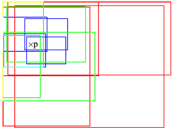
Figure 1. Illustration of three window sizes (respectively plotted in red, green, and blue) with an overlap rate of 50%. Any point p in the image domain belongs to a subset of windows of different size.

A static camera configuration is assumed, as it is the usual situation in the targeted applications, but extension to a mobile camera could be considered, for instance by compensating beforehand for the dominant image motion due to the camera motion. In order to minimize the computational load, we extract first the binary mask of moving objects in every frame by means of a motion detection algorithm. To this end, we use our motion detection method by background subtraction described in Crivelli et al. (2011) which also built upon (Veit et al., 2011). We denote by ϒ(t) the set of moving pixels extracted at time instant t, with ϒ(t) ⊂ Ω.

We assume that affine motion models are sufficient to represent image motion with the view of anomalous motion detection. The velocity vector of point p ∈ ϒ(t) at time instant t given by the affine motion model of parameters θ(t) = (b₁(t), a₁(t), a₂(t), b₂(t), a₃(t), a₄(t)), reads

$w_{\theta (t)}(p)=\left(\begin{array}{c}{u}_{\theta (t)}(p)\\ {\nu }_{\theta (t)}(p)\end{array}\right)=\left(\begin{array}{c}{b}_1(t)+a_1(t)x+a_2(t)y\\ b_2(t)+a_3(t)x+a_4(t)y)\end{array}\right).$ (1)

We will even further assume that, at the proper scale, it can be represented by one of the three following specific affine motion models: translation (T), scaling (S), and rotation (R). As explained above, the three types of 2D motion models are computed in a collection of predefined windows. We use the robust estimation method (Odobez and Bouthemy, 1995) implemented in the publicly available Motion2D software¹ to compute these parametric motion models.

Let us denote by $\mathcal{W}\left(p\right)$, $\mathcal{M}\left(p,t\right)$, and Θ(p, t), respectively, the set of windows from the collection 𝒲 containing point p, the set of motion models computed at time instant t within the windows of $\mathcal{W}\left(p\right)$ and supplying candidate velocity vectors at p, and the associated set of parameter values of these motion models. We have $\left|\mathcal{M}\left(p,t\right)\right|=3\left|\mathcal{W}\left(p\right)\right|$, where |.| denotes the set cardinality, since three 2D motion models (T, R and S, as defined above) are computed in each window of $\mathcal{W}\text{(}p\text{)}$. We have $\mathrm{\Theta }\left(p,t\right)=\left\{{\theta }_k\left(t\right),k=1\dots \mathrm{|}\mathcal{M}\left(p,t\right)\mathrm{|}\right\}$. With the aforementioned choices on the number of window sizes and the overlap rate, we have $\left|\mathcal{W}\left(p\right)\right|=4\times 4=16$ and $\left|\mathcal{M}\left(p,t\right)\right|=48$.

In the sequel, for the sake of notation simplicity, we will drop the reference to time instant t. We aim to find the most relevant motion model at p ∈ ϒ among the candidates specified by Θ(p). We take the displaced frame difference as fitting variable to test each motion model k of $\mathcal{M}\left(p\right)$ at p:

$ϵ\left(p,{\theta }_k\right)=I_{t+1}\left(p+w_{{\theta }_k}\left(p\right)\right)-I_t\left(p\right),$ (2)

where I_t(p) denotes the intensity at p at time instant t, and $w_{{\theta }_k}\left(p\right)={\left(u_{{\theta }_k}\left(p\right),v_{{\theta }_k}\left(p\right)\right)}^T$ is the velocity vector given by the motion model k at p. Let us specify expression (1) for the three motion types. For the T-motion type,

$w_{{\theta }_k}\left(p\right)={\left(b_{1,k},b_{2,k}\right)}^T\text{with}{\theta }_k=\left(b_{1,k},b_{2,k}\right);$

for the S-motion type,

$w_{{\theta }_k}\left(p\right)={\left(b_{1,k}+a_{1,k}x,b_{2,k}+a_{1,k}y\right)}^T,{\theta }_k=\left(b_{1,k},b_{2,k},a_{1,k}\right);$

and for the R-motion type,

$w_{{\theta }_k}\left(p\right)={\left(b_{1,k}+a_{2,k}y,b_{2,k}-a_{2,k}x\right)}^T,{\theta }_k=\left(b_{1,k},b_{2,k},a_{2,k}\right).$

3.2. Selection among the Motion Model Candidates

The optimal motion model at p should best fit the real (unknown) local motion at p while being of the lowest possible complexity. We consider a local neighborhood ν(p) centered in p, and we exploit the fitting variable (2), which is likely to be close to 0 for the correct velocity vector exploiting the intensity constancy constraint as done for optical flow computation (Fortun et al., 2015). Let us assume that the $ϵ\left(q,{\theta }_k\right)$’s are independent identically distributed (i.i.d.) variables over points q ∈ ν(p) ∩ ϒ and follow a zero-mean Gaussian law of variance ${\sigma }_k^2$. Then, we can write the joint likelihood in the neighborhood ν(p) for each motion model k:

$\varphi \left(p,{\theta }_k\right)=\frac{1}{{\sqrt{2\pi {\sigma }_k^2}}^{|\nu \left(p\right)\cap \Upsilon |}}{\displaystyle \prod _{q\in \nu (p)\cap \Upsilon }}\exp -\frac{ϵ{\left(q,{\theta }_k\right)}^2}{2{\sigma }_k^2}.$ (3)

The variance ${\sigma }_k^2$ is estimated from the inliers of the motion model k within the window used for robustly estimating the motion model k. To penalize the complexity of the motion model, i.e., the dimension of the model given by the number of its parameters, we resort to the Akaike information criterion (AIC) with a correction for finite sample sizes (Cavanaugh, 1997). The correction is especially useful when the sample size is small, which is precisely the case here for the neighborhood ν(p). The penalized criterion writes as follows:

$\mathit{AICc}\left(p,{\theta }_k\right)=-2\ln \left(\varphi \left(p,{\theta }_k\right)\right)+2{\eta }_k+\frac{2{\eta }_k\left({\eta }_k+1\right)}{|\nu \left(p\right)\cap \Upsilon |-{\eta }_k-1},$ (4)

where η_k is the dimension of the motion model k, that is, η_k = 2 for T-motion model, and η_k = 3 for S- and R-motion models. Finally, the optimal motion model $\widehat{k}$ at p is

$\widehat{k}\left(p\right)=\text{arg}\underset{{\theta }_k\in \mathrm{\Theta }\left(p\right)}{\min }\mathit{AICc}\left(p,{\theta }_k\right),$ (5)

which minimizes criterion (4).

From the motion models selected at pixels p ∈ ϒ, we obtain the affine flow $\left\{w_{{\theta }_{\widehat{k}\left(p\right)}}\left(p\right),p\in \Upsilon \right\}$.

3.3. Determination of Motion Classes

We have now to assign to each p ∈ ϒ its motion class. The motion classes will be used to compute the motion descriptors which are the input of our anomalous motion detection method. As explained in subsection 3.2, we have selected the right motion model at each point p ∈ ϒ among the estimated motion model candidates with the penalized likelihood given by the corrected Akaike information criterion for small sample sets defined in equation (5).

As already stated, the different image motions are assumed to be well captured by three affine motion types: translation (T), scaling (S), and rotation (R), in a view-based representation. Motion classes are straightforwardly inferred from the motion types as summarized in Tables 1 and 2. More specifically, the translation type is subdivided into motion classes indicating the direction of the translation in the image, since we have adopted a motion representation corresponding to the camera view point. The scaling type is split in two classes, called Convergence and Divergence, according to the sign of the divergence coefficient. Finally, the rotation type is subdivided into Clockwise and Counterclockwise motion classes. Aiming for other crowd analysis tasks than anomaly detection, the crowd motion classification introduced in Basset et al. (2014) comprised only four translation classes (i.e., North, East, South, and East). Here, we introduce a finer orientation quantization with eight translation directions. Indeed, we need a finer characterization of the movement for anomalous motion detection. We come up with a set of twelve motion classes, denoted by Γ = {γ_l, l = 1, … 12}. From now on, the motion classes will be represented in the figures by the color codes given in Table 1.

TABLE 1

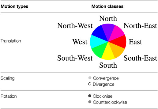
Table 1. Definition of motion types, motion classes, and color codes.

TABLE 2

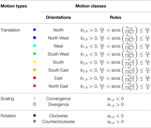
Table 2. Rules for determining motion classes from motion types.

The motion classification map $\mathcal{L}\left(t\right)$ is determined by applying the rules summarized in Table 2. They are based on the signs of the parameters of the selected motion models and on simple functions of these parameters. Each $\mathcal{L}\left(p,t\right)$ value is one of the twelve motion classes γ_l of the set Γ. This is illustrated on Figure 2. In contrast to Basset et al. (2014), we do not regularize $\mathcal{L}\left(t\right)$ by a vote procedure, since we precisely aim to detect local anomalous motion. The local motion information must not be smoothed out. If we process an image sequence of 𝒯 successive images, we come up with $\mathcal{T}-1$ successive motion classification maps $\mathcal{L}\left(t\right),t=1\dots \mathcal{T}-1$.

FIGURE 2

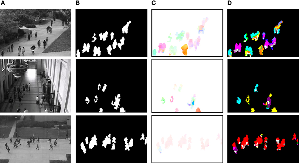
Figure 2. Overview of the computation of the labeled affine flow in several real video sequences. (A) Input images. (B) Motion detection maps ϒ(t). (C) Affine flow deduced from the selected motion models, colored according to standard code for optical flow maps, which is the continuous version of the quantized color code used for Translation classes provided in Table 1. (D) Map ℒ(t) of motion classes for each pixel, colored according to Table 1.

We coin the term Labeled Affine Flow (LAF) to emphasize that, from the selected motion model at p ∈ ϒ, we have not only computed an affine flow vector at p but have jointly determined its motion class. The labeled affine flow is defined at each time instant t of the video sequence by $\left\{\left(w_{\theta {\left(t\right)}_{\widehat{k}\left(p\right)}}\left(p\right),\mathcal{L}\left(p,t\right)\right),p\in \Upsilon \left(t\right)\right\}$.

A possible extension to the classification process would be to include more motion classes (e.g., by first adding the motion type TRS—Translation plus Rotation plus Scale—and then, corresponding motion classes). For our target application, however, addressing too many motion classes would have detrimental effects. In particular, it might affect the statistical relevance of motion class histograms and make the discrimination of local anomalies difficult. It would require more available data with all the possible motion combinations.

4. Detection and Localization of Anomalous Motion

Our anomalous motion detection-and-localization method relies on local motion classes derived from the pixelwise selected motion types. We compute block-based motion-weighted histograms of these motion classes as motion descriptors to characterize local motions. We use non-overlapping blocks as illustrated in Figure 3. If required, overlapping blocks could be used as well to increase the spatial accuracy of the anomalous motion detection at the expense of computation load, down to a pixelwise detection with one-pixel stride in the block generation. Then, we adopt a density-based measure in the histogram space to detect anomalous motion. The pipeline is explained in detail hereafter.

FIGURE 3

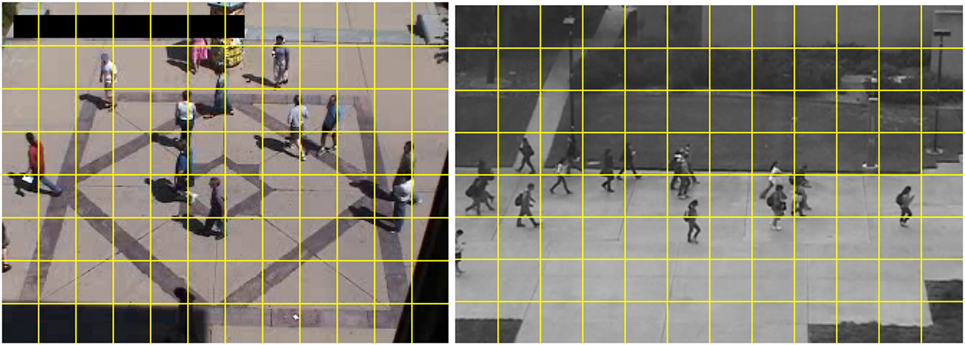
Figure 3. Spatial blocks are introduced to allow localization of anomalous motion. The images are respectively taken from the UMN and UCSD datasets.

4.1. Local LAF Histograms

As noted in Section 2, feature-based methods for anomaly detection that benefit of direct use of spatial information achieve better performance. For this purpose, we split the image, and consequently the scene since the camera is static, in spatial blocks ${\mathcal{B}}_i$, with i = 1 … B. This subdivides the anomalous motion detection task in multiple sub-problems (see Figure 3). We introduce an original motion histogram which we call LAF histogram. The LAF histogram is computed for every block ${\mathcal{B}}_i$ at time t, and is denoted by $h_i^t$. The LAF histogram corresponds to a weighted motion class histogram. More specifically, the LAF histogram $h_i^t$ is constructed by summing a function ψ(p, t, l) over block ${\mathcal{B}}_i$ within a short time interval around time instant t. We define ψ(.) as follows:

$\psi \left(p,t,l\right)=\left\{\begin{array}{cc}||w_{{\theta }_{k_l}}\left(p,t\right){||}_2\hfill & \text{if}\mathcal{L}\left(p,t\right)={\mathrm{\gamma }}_l,\hfill \\ 0\hfill & \text{otherwise},\hfill \end{array}\right.$ (6)

where k_l denotes the motion model selected at p with equation (5), and associated with the motion class γ_l. As defined by equation (6), the weight to be added in bin l of the histogram is the magnitude of the affine flow vector at p. Thus, we simultaneously take into account both the motion magnitude and the motion class to detect anomalous motion. As aforementioned, affine motion magnitude was not exploited in Basset et al. (2014). For each bin l of the histogram, we set:

$h_i^t\left(l\right)={\displaystyle \sum _{p\in {ℬ}_i}}{\displaystyle \sum _{\tau =t-1}^{t+1}}\psi \left(p,\mathrm{\tau },l\right),$ (7)

involving the previous (t − 1) and following (t + 1) frames to build the histogram at time t. This procedure enables us to specify short-term temporal behaviors in a given block. The motion magnitude is used to weight the importance of a given motion class (or bin of the histogram). In this way, we manage to capture several essential aspects of motion in a single descriptor, allowing us to distinguish anomalies by their speed and their movement direction as well. It is true that a small fast moving object and a large slow one may lead to similar histograms if they undergo exactly the same type of motion and if the ratios in speed and size are strictly equal, which has however a very low probability to occur.

4.2. Dedicated LAF Histogram Distance

We now specify the appropriate distance to compare two LAF histograms. Let us take two LAF histograms computed in the same block ${\mathcal{B}}_i$ for two different images and referenced as α and β. They could be the test histogram and the training one for instance. As a matter of fact, this distance will combine two distances, since we first separate the histograms in two sub-histograms. The first one involves the eight classes of translation motion, and the second one involves the four classes related to scaling and rotation motions. This will be motivated right below. The two sub-histograms are denoted by κ_i and ζ_i, respectively.

For the translation-related sub-histogram, we adopt the modulo distance D_mod(⋅, ⋅) introduced in Cha and Srihari (2002) for circular histograms. This is precisely the case for the translation sub-histogram, since the eight translation classes are defined by compass orientations (see Table 1). There is no closed-form way to compute the modulo distance, but an algorithm is available, the pseudocode of which can be found in Cha and Srihari (2002). The modulo distance plays a key role as it is higher between opposite directions that between adjacent ones. It can truly emphasize discrepancy and closeness between motion translation classes, and it is less sensitive to orientation quantization. On the other hand, the sub-histograms related to scaling and rotation motion classes are compared with a L₁ distance. We found that L₁ distance was the best choice after experimentally comparing several usual histogram distances. The overall histogram dissimilarity measure between two LAF histograms $h_i^{\alpha }$ and $h_i^{\beta }$ is then defined as follows:

$D\left(h_i^{\alpha },h_i^{\beta }\right)=D_{\mathit{mod}}\left({\mathrm{\kappa }}_i^{\alpha },{\mathrm{\kappa }}_i^{\beta }\right)+D_{L_1}\left({\mathrm{\zeta }}_i^{\alpha },{\mathrm{\zeta }}_i^{\beta }\right),$ (8)

with equally weighted summands, since the ranges of the modulo and L₁ distances are similar as explained in Cha and Srihari (2002).

4.3. Local Outlier Factor

We face a specific situation for formulating the anomalous motion detection criterion. We have no prior models on what should be both normal and abnormal behaviors. Training a classifier could be a possibility; it is easy to collect training examples for normal behaviors. However, we have usually few available anomalous motion examples, they can be of different kind, and in particular they may be unexpected. Furthermore, we want that our method can be applied online as well, without any previous learning stage. This advocates for a purely data-driven decision process to detect anomalous motion. A LAF histogram corresponding to anomalous motion should be an outlier in the feature space of LAF histograms, where all computed LAF histograms are collected, since the large majority of LAF histograms are likely to correspond to normal behaviors. An outlier can be characterized by its distance to clusters of normal behavior. However, this would require to perform clustering in a high-dimensional space without knowing the number of clusters and their respective shape (inner distribution). Then, a more attractive approach is to compare the local density of features (i.e., histograms) around the test histogram with the local feature densities of its nearest neighbors.

To do this, we resort to the local outlier factor (LOF) which is precisely a measure to discriminate anomalous data in a dataset. LOF was proposed to detect anomalies in the e-commerce field (Breunig et al., 2000). It has subsequently been used to detect anomalies for other kinds of problems, such as network intrusions (Lazarevic et al., 2003). However, LOF has not been exploited so far for solving computer vision problems. We will demonstrate its utility for anomalous motion detection in videos.

The rationale behind the LOF measure is that detecting outliers can be achieved by identifying points of a certain feature space that have low data density around them with respect to their neighbors. This approach allows one to specify abnormality in a local and relative way. It is thus quite flexible. This is illustrated in Figure 4, which includes two clusters, C₁ and C₂, and a few other data points, such as $h_1^{{\alpha }_1}$ and $h_j^{{\alpha }_2}$, supposed to be outliers (i.e., anomalous motion for our problem). If we merely perform thresholding on the distance of the data point to the cluster centroids, it may be tricky to set the threshold value and lead to errors. Indeed, several points of cluster C₁ could be for instance incorrectly labeled as anomalous, or conversely it could be the case that $h_j^{{\alpha }_2}$ may be interpreted as an inlier.

FIGURE 4

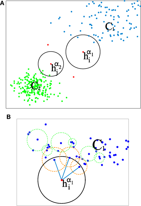
Figure 4. (A) Illustrative case where a dataset is shaped mainly in the form of two clusters (data points in green and blue), with a few of clear outliers in red, including $h_i^{{\alpha }_1}$ and $h_j^{{\alpha }_2}$. In our case, data points in the feature space for a single block are LAF histograms of weighted motion classes. (B) Detail for the outlier data point $h_i^{{\alpha }_1}$, where the local reachability density of the data points is encoded with circles. Regarding the neighborhood of k-nearest histograms, k = 3 in this illustration. The outlier point is surrounded by a circle (in blue) that is clearly bigger that the ones of their neighbors (circles in orange).

By contrast, using the LOF measure, an “outlierity” measure is assigned to every point in the dataset, and it does not require to determine any cluster. This measure is calculated as the average local density attached to data points within its neighborhood divided by its own local density. This notion is illustrated in Figure 4B, by encoding the density measure as a circle that contains the k-nearest neighbors of a given point. The larger the circle, the smaller the density measure. It can be observed that inliers are surrounded by smaller circles than the outlier points. The formal definition of this density is supplied later on in this section. Thus, if a data point of the feature space is assigned a low density compared to data points in its neighborhood, its outlierity measure is higher.

The neighborhood of a data point in the feature space is given by its k-nearest neighbors for the distance of equation (8). In this sense, the neighborhood geometry is locally adaptive. Although the distance of a tested data point to a “normal” point may be smaller that the distance between two other “normal” points, the test data point can still be classified as outlier/anomalous, if its most proximal neighbors depict a higher density. As an example, in Figure 4, it can be seen that although the distance between data point $h_j^{{\alpha }_2}$ and points of cluster C₂ is similar to the distance between pairs of data points in cluster C₁, $h_j^{{\alpha }_2}$ can still be detected as outlier/anomalous, since its density is being compared to data points that belong to C₂ mainly. The same reasoning can be applied to data points of cluster C₁, allowing them to be labeled as inlier/normal.

More formally, we need first to introduce the reachability distance (Breunig et al., 2000) of a histogram $h_i^{\alpha }$ from another histogram $h_i^{\beta }$:

${\phi }_k\left(h_i^{\alpha },h_i^{\beta }\right)=\max \left(D\left(h_i^{\beta },h_i^{k\left(\beta \right)}\right),D\left(h_i^{\alpha },h_i^{\beta }\right)\right),$ (9)

where k(β) denotes the k-th nearest neighbor of β, and D(⋅, ⋅) the distance introduced in equation (8). Let us stress that φ_k(⋅, ⋅) is not a real distance since it is not symmetric. Hence, ${\phi }_k\left(h_i^{\alpha },h_i^{\beta }\right)$ is not expected to be equal to ${\phi }_k\left(h_i^{\beta },h_i^{\alpha }\right)$.

We denote the set of k-nearest neighbors of a given histogram $h_i^{\alpha }$ by ${\mathcal{N}}_k\left(h_i^{\alpha }\right)$. The local reachability density ${\rho }_k\left(h_i^{\alpha }\right)$ is defined as the inverse of the average reachability distance of the histogram $h_i^{\alpha }$ from its neighbors (Breunig et al., 2000):

${\rho }_k\left(h_i^{\alpha }\right)={\left(\frac{1}{k}{\displaystyle \sum _{h_i^{\eta }\in {𝒩}_k(h_i^{\alpha })}}{\phi }_k\left(h_i^{\alpha },h_i^{\eta }\right)\right)}^{-1},$ (10)

since the cardinality of ${\mathcal{N}}_k\left(h_i^{\alpha }\right)$ equals k. Let us remind that ${\phi }_k\left(h_i^{\alpha },h_i^{\eta }\right)$ is the reachability distance of $h_i^{\alpha }$ from $h_i^{\eta }$, not to be confused with ${\phi }_k\left(h_i^{\eta },h_i^{\alpha }\right)$.

The local outlier factor LOF^k (upper script k expresses the use of k-nearest neighbors) is then defined to compare the local reachability densities of a given histogram with respect to its own neighbors as follows (Breunig et al., 2000):

${\mathit{LOF}}^k\left(h_i^{\alpha }\right)=\frac{{\sum }_{h_i^{\eta }\in {\mathcal{N}}_k\left(h_i^{\alpha }\right)}{\rho }_k\left(h_i^{\eta }\right)}{\left|{\mathcal{N}}_k\left(h_i^{\alpha }\right)\right|{\rho }_k\left(h_i^{\alpha }\right)}.$ (11)

In other words, the local outlier factor captures the local reachability density ratio between the neighbors of a given histogram and itself. It produces values that are close to one if the average density of its neighbors is similar to its own. Conversely, higher values indicate possible outliers.

4.4. Test for Detecting Anomalous Motion

Our goal is to make a classification for every block in every frame of the video sequence in two classes, namely, “normal motion” and “anomalous motion.” As explained in Section 1, the large majority of these are likely to correspond to “normal motion.” In order to perform this classification, we measure the LOF of the current LAF histogram in a given block and compare it to a threshold.

As explained in the previous section, the LOF measure outputs a value by comparing the local density around the test LAF histogram in the LAF histogram collection, with respect to the density of its nearest k-neighbors. The LOF measure is constructed independently for each block ${\mathcal{B}}_i$.

Specifically, we decide that a LAF histogram $h_i^t$ computed in block ${\mathcal{B}}_i$ at time instant t, corresponds to an anomalous motion if

$\mathit{LO}{F}_i^k\left(h_i^t\right)>{\mathrm{\lambda }}_i,$ (12)

where $\mathit{LO}{F}_i^k$ is the local outlier factor computed in the subspace of LAF histograms computed over time in block ${\mathcal{B}}_i$ and by taking into account the nearest k-neighbors.

Each λ_i is automatically inferred from a p-value, denoted by ξ, on specific statistics of every block ${\mathcal{B}}_i$. In fact, we want λ_i to control the number of wrongly classified blocks. In order to do this, we exploit the computed LOF values corresponding to normal motion (for instance, using a training dataset comprising only normal motion cases). Thus, for every block ${\mathcal{B}}_i$, a distribution of LOF values is stored. As shown in Pécot et al. (2015), we can set:

${\mathrm{\lambda }}_i={\mu }_i+{\sigma }_i∕\sqrt{\xi },$ (13)

where, for each ${\mathcal{B}}_i$, μ_i and σ_i are the trimmed mean and the winsorized variance (Huber, 1981) computed from the empirical distribution of the stored LOFs, while discarding the 20% more extreme values in order to reduce the effect of spurious LAF histograms. Equation (13) does not imply that the distribution of LOF values is close to a Gaussian distribution, and in practice, it might by far from it. This relationship is merely inferred from equation (12) using the Chebyshev inequality (Pécot et al., 2015).

Nevertheless, it is convenient to add further filtering as the initial classification output can be noisy. This is done by adding a post-processing step to our method. Indeed, anomalous motion is likely to be persistent for a (short) period of time. For the anomalous motion localization in our pipeline (decision at the block level), a percentile filter is applied on the classification output to accept or reject anomalous motion candidates. We take a temporal neighborhood of the block including the previous and next frames, as drawn in Figure 5. The neighborhood shape allows us to take into account that anomalous motion blocks may shift between two frames following the outlier moving object displacement. The classification label of block ${\mathcal{B}}_i$ is updated to the value of the 16th element of the binary vector formed by the initial classification labels (1 for anomalous motion, 0 for normal motion) of its space–time neighborhood. This vector comprises 19 components, that is the 18 labels of the space–time neighborhood and the initial label of the block, organized in ascending order.

FIGURE 5

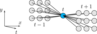
Figure 5. Illustration of the temporal block neighborhood for anomalous motion detection-and-localization filtering. Each block has 18 neighbors.

As for frame-level decision, one frame is said to contain anomalous motion, if at least one of its blocks is detected as such. On the other hand, for the frame-level anomalous motion detection, a temporal median filter of size 7 is applied on the frame-classification output. This classification, although simple, offers satisfactory results, as the underlying block-based LAF histograms capture very well different aspects of the visual data.

5. Experimental Results

We present several experiments to assess the performance of our anomalous motion detection method. At the end of this section, in subsections 5.7 and 5.8, we will demonstrate how the two main ingredients of our method, that is, the LAF histograms and the LOF criterion, contribute to its overall performance.

We report comparative results on three datasets: UMN dataset (Papanikolopoulos, 2005), PETS2009 dataset (Ferryman and Shahrokni, 2009), and UCSD dataset (Li et al., 2014). We did not run codes of other methods, but we only collected results when available in previously published papers. The two first datasets depict global motion anomalies, that is, people in the scene all together adopt a new dynamic behavior at the same time instant, like suddenly running. The UCSD dataset is of a different kind. It involves local anomalies, but above all, anomalies are due to the type of both object and motion. Indeed, anomalies are formed by cyclists and skateboarders riding, or vehicles driving among pedestrians walking on a campus path. Thus, this dataset is not truly intended to assess anomalous motion detection on its own, and accordingly, the most performing methods are those exploiting both appearance and motion (Antic and Ommer, 2011; Li et al., 2014). Yet, this dataset is a popular one in crowd anomaly detection, so we believed that it was worth evaluating our method on the UCSD dataset as well, in order to show the usefulness of our anomalous motion detection method for this task, and by doing so its versatility. Nevertheless, for a fair assessment, we will compare our method with motion-based anomaly detection methods only. Indeed, our end goal is not to define a method dedicated to crowd anomaly detection, but a generic method for anomalous motion detection. The fourth experiment will deal with two video sequences of crowded scenes which exhibit local anomalous motion, and results will be only visually assessed.

There are different ways to compute normal LAF histograms to populate the LAF histogram space and correctly compute the LOF criterion. If we are dealing with densely enough crowded scenes where the large majority of people undergo normal behavior and only a few local anomalous motion may appear, we can apply the online version of our method. It means that the reference LAF histograms $h_i^{\beta }$ can be computed in the very same image at every time t, since most of blocks ${\mathcal{B}}_i$ include normal behavior. If the anomalous motion corresponds to a global sudden change in dynamic behavior, normal LAF histograms can be computed in the first part of the video sequence. We will specify for each experiment the way LAF histograms corresponding to normal motion are computed.

For all the experiments, we set k = 7 for the k-nearest neighbors in the LOF computation. This value was selected by cross-validation on the UCSD dataset, which provides with complete per-pixel annotation. The block size is defined by the grid partition. We found that this parameter does not vary much the results, as long as the blocks cover an area that is similar in size to the expected actors of the normal events. For the UNM and UCSD dataset, we fix the grid size to 12 × 8 blocks. For the rest of the presented experiments we use 8 × 8.

Objective comparison will be based on two performance criteria specified by previous work, namely, frame-level and pixel-level ones. The set of compared methods may vary depending on the dataset, according to availability of reported experimental results (performance numbers and ROC curves). The pixel-level criterion establishes that the frame detected anomalous is considered correctly classified if at least 40% of the truly anomalous pixels are detected. This procedure should not be confused with a truly pixelwise evaluation, but it ensures a minimal precision–recall balance. This pixel-level criterion was introduced in Mahadevan et al. (2010), and it has been widely adopted in the crowd anomaly detection literature. The frame-level criterion simply acknowledges a correct classification if at least one true anomaly is detected in the frame.

5.1. Experiments on the UMN Dataset

The UMN dataset includes eleven sequences of sudden escape events corresponding to three scenes (indoor and outdoor, see Figure 6 for samples). The videos depict groups of people freely walking around open spaces and performing ordinary actions inside a building lobby, which represents normal behaviors. The anomalies occur when the people start running until they get out of view. This corresponds to a global anomalous motion case. Nevertheless, we are still able to localize where anomalous motion occur in every image. From the total of 7740 frames of the dataset, 1431 depict escaping behaviors, that is, correspond to anomalous motion. Reference LAF histograms are then computed in each block ${\mathcal{B}}_i$ containing moving pixels, of the first 6000 frames displaying normal behavior.

FIGURE 6

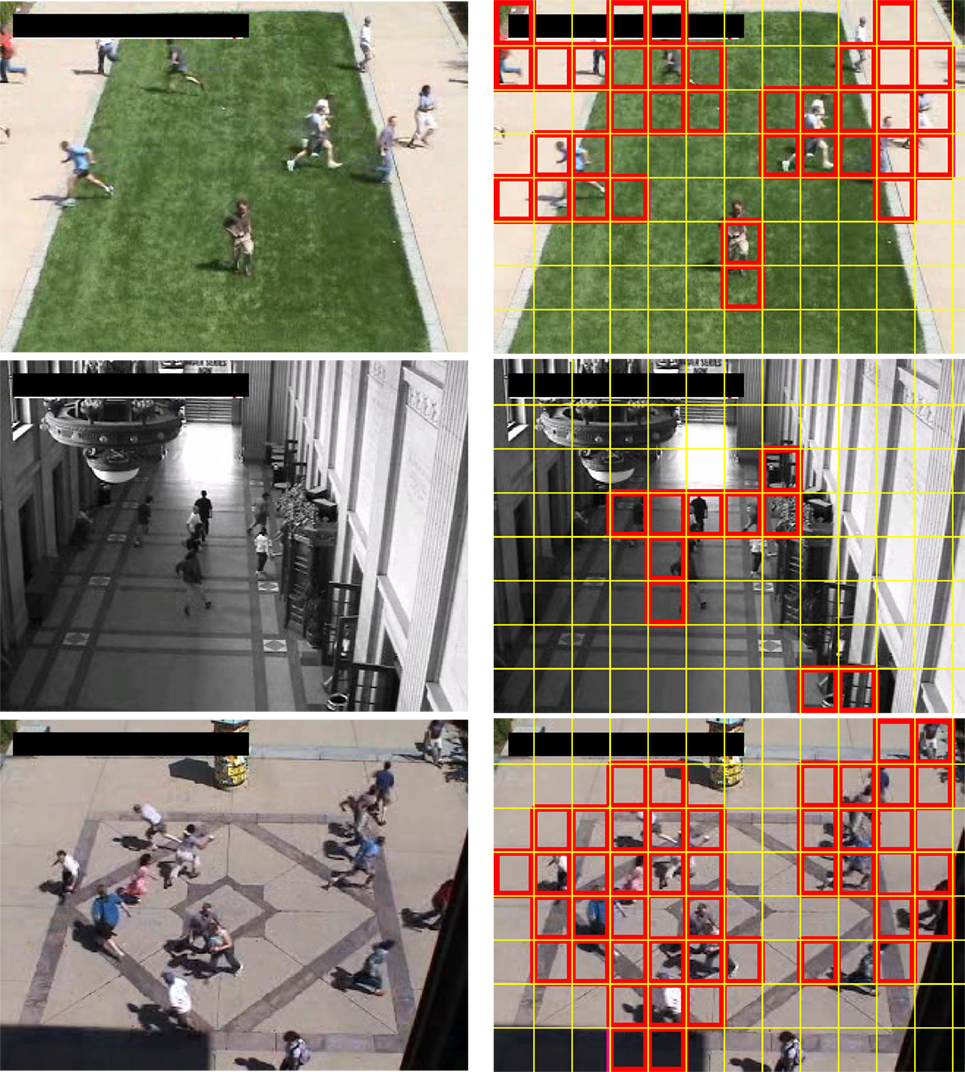
Figure 6. Left column: original samples of the UMN dataset. Right column: blocks where anomalous motion detection is localized by our method are framed in red. From top to bottom: examples respectively from scene 1, scene 2, and scene 3 of the UMN dataset.

We report comparative results with the following motion-based anomaly detection methods: the method based on sparse reconstruction error (SRC) (Cong et al., 2013) which exploits multi-scale histograms of optical flow, the method relying on chaotics invariants (CI) (Wu et al., 2010), the method involving the social force model (SF) (Mehran et al., 2009), the method built upon scan statistic (SS) (Hu et al., 2013), and the method introducing motion influence maps (MIM) (Lee et al., 2015). Sample visual results are gathered in Figure 6. Available ROC curves are plotted in Figure 7. The frame-level criterion is used for the UMN dataset. We report the area under the ROC curve and the equal error rate (EER) in Table 3. The EER corresponds to equal false positives and false negatives. Numbers are taken from Mahadevan et al. (2010) and Zhang et al. (2016) for the other methods. To compute the frame-level evaluation in our method, we consider that a frame is anomalous if at least one block in it is labeled as such. From Table 3 and Figure 7, we can conclude that our method is very competitive. It provides the second best result regarding EER, and it is close to the two best ones regarding AUC. Furthermore, it outperforms other motion-based methods MIM (Lee et al., 2015), SS (Hu et al., 2013), and SF (Mehran et al., 2009), when examining results scene by scene.

FIGURE 7

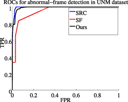
Figure 7. ROC curves for SRC (Cong et al., 2013), SF (Mehran et al., 2009), and our method on the UMN dataset (TPR stands for True Positive Rate and FPR for False Positive Rate).

TABLE 3

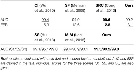
Table 3. Anomalous motion detection performance on the UMN dataset.

5.2. Experiments on the PETS2009 Dataset

Each one of the scenarios of the PETS2009 dataset contains four sequences from different points of view of the scenes. We used the same number of training frames as reported in Wu et al. (2014), that is 30 for the first scenario and 100 for the second one, to compute the LAF histograms of normal behavior. Anomalous motion in the two scenarios consists of people who suddenly start running at some time instant of the videos.

We present results for the frame-level accuracy criterion, more specifically the number of correctly classified frames over the total of frames, on two selected scenarios of the PETS2009 dataset (Figure 8), as proposed in Wu et al. (2014). We compare our method with four different methods: chaotic invariants (CI) (Wu et al., 2010), the social force model (SF) (Mehran et al., 2009), the force field method (FF) (Chen and Huang, 2011), and the Bayesian model (BM) described in Wu et al. (2014). Our method supplies state-of-the-art results on this dataset as shown in Table 4. Indeed, our method has the best average scores for the two scenarios. This experiment also demonstrates that our method is stable and remains reliable when only few training samples are available.

FIGURE 8

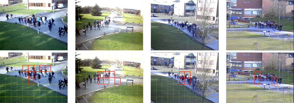
Figure 8. Top row: sample images from the PETS2009 dataset. Bottom row: blocks where anomalous motion is localized by our method are framed in red.

TABLE 4

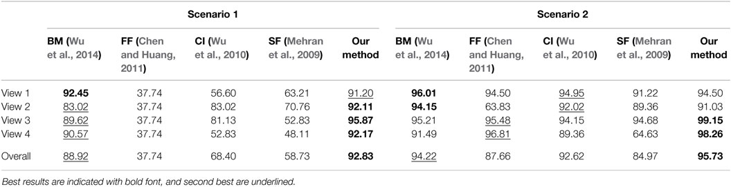
Table 4. Frame-level accuracy (%) for several methods on sequences of PETS2009 dataset.

5.3. Experiments on the UCSD Dataset

The UCSD dataset was introduced in Mahadevan et al. (2010) and consists of videos of sparse crowds divided in two scenarios. We used the ped1 subset (Figure 9) where the normal behaviors are people walking through the campus scene at a normal speed, toward and away from the camera. As aforementioned, anomalies in this dataset are composed mainly by moving cars, skateboarders, and cyclists, among others. Clearly, the anomalies of this dataset are not only specified by their motion but also by the involved object (car, bike, skate board, etc.). This explains that methods exploiting appearance features may have superior performance as the Video Parsing (VP) method (Antic and Ommer, 2011), and the method based on a mixture of dynamic textures (MDT) (Li et al., 2014).

FIGURE 9

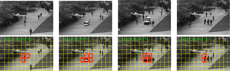
Figure 9. Top row: sample images of the UCSD dataset. Bottom row: blocks containing anomalies detected by our method are framed in red. From left to right: cyclist, vehicle, vehicle, cyclist.

The ped1 scenario contains 36 testing and 34 training videos, as well as labeled ground truth at the frame level and pixel level. We use the training sequences, which are composed only by normal events, to initialize the reference LAF histogram space. Results on this dataset are summarized by the area under the ROC curve (AUC). At the frame level, error measures rely on a frame-by-frame binary classification, while at the pixel level, the measures are based on ground truth masks which are partially provided by the authors of the dataset (Mahadevan et al., 2010), and extended to the full dataset by a more recent work (Antic and Ommer, 2011). We will respectively refer to them as partial and full ground truth from now on.

We first present visual results of our method in Figure 9, where we can observe that blocks containing anomalies are accurately localized. AUC values are given in Table 5 for three motion-based methods AD (Adam et al., 2008), SF (Mehran et al., 2009), and SS (Hu et al., 2013), and for our method (including also a multi-grid extension which is explained later on). Since the pixel-level evaluation is not available for all the motion-based methods on the full ground truth, we supply a complementary comparison on the partial ground truth in Table 6.

TABLE 5

Table 5. Anomaly detection performance (AUC) on the UCSD dataset (ped1) at the frame level evaluated on the full ground truth (Antic and Ommer, 2011).

TABLE 6

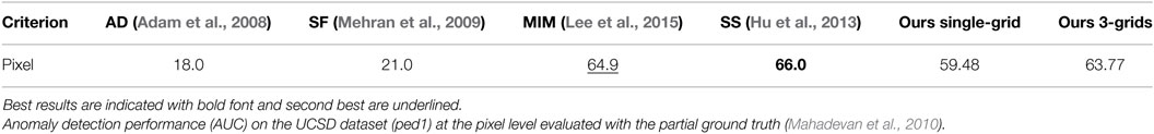
Table 6. Comparison with motion-based methods.

Our anomaly localization output is given as a binary variable for each block ${\mathcal{B}}_i$ at every time t. However, in order to compute the ROC curves, we make use of moving object masks ϒ(t) computed before the determination of the per-pixel motion classes. We intersect them with blocks labeled as anomalous. Thus, for the pixel-level evaluation of our method, the anomaly detection mask at each time instant t, is given by ${\cup }_i\left(\Upsilon \left(t\right)\cap {\mathcal{B}}_i\right)$, for the ${\mathcal{B}}_i$’s labeled as anomalous.

Since our per-block anomaly detection output depends on how anomalous events are positioned within the fixed block grid, our method may fail to detect an anomaly (or at least part of its support), when the anomaly lies astride two or more blocks. In order to overcome this problem, we can extend our method by combining additional output of our algorithm computed over two more grids. These grids are horizontally and vertically displaced versions of the original one by half the length of a single block. The combination is simply achieved by intersecting all the blocks detected as anomalous in the three grids, with the motion detection support at each frame.

In this demanding dataset, our method shows strengths that enable it to detect most anomalies. For instance, Figure 9 (4th column) shows correct anomaly detection of a cyclist, which is a difficult case because it is moving at a similar speed as the walking people. Let us also stress that from the perspective of the camera, the cyclist looks not that different from a normal pedestrian. However, the difference in the leg motion of the cyclist (or the skateboarders in other sequences) with respect to pedestrians is captured by the LAF histograms. In fact, the normal walking usually involves Scaling motion classes, which is not the case of the cyclist.

Our method supplies competitive results in this dataset as reported in Table 5. Our method is the second top performing one among motion-based methods for the frame-level criterion on the full ground truth dataset. For the pixel-level evaluation, only results on the partial ground truth dataset are available for other motion-based methods. They are given in Table 6. This score partly allows for localization assessment. We can notice that our method exhibits a very significant performance improvement of almost 40 points with respect to the motion-based methods (Adam et al., 2008; Mehran et al., 2009), while being (for the 3-grid version) on par with MIM (Lee et al., 2015), which is a recently published method developed in parallel to ours, and slightly inferior to SS (Hu et al., 2013). However, in contrast to ours, the latter cannot actually deliver results on the fly, since it is based on a two-round scanning which needs the global distribution of the likelihood test values computed in the first scan of the video.

5.4. Additional Experiments on Videos with Local Anomalous Motion

5.4.1. Wrong Way Video

The Wrong way video contains 445 frames acquired by a camera pointing toward a crowd passing by. A person is walking in the opposite direction of the crowd. Thus, this interval comprises the anomalous event. We processed the video from frame 160 to frame 223. We split the training set into two parts to capture normal behaviors. For the lower half of the scene, we use the interval of frames starting from frame 30 to frame 75. For the upper part of the scene, we take the interval of frames that goes from frame 235 to frame 280. Sample images with overlaid results are shown in Figure 10. The interaction with the other people, of the man pushing his way through the crowd, makes the other people modify their own motion. They rotate to avoid him, and consequently, participate to the anomalous event. Visual results provided in Figure 10 show that our block-based detection method performs well and is able to accurately detect both the anomalous motion of the man and of the people he is in contact with.

FIGURE 10

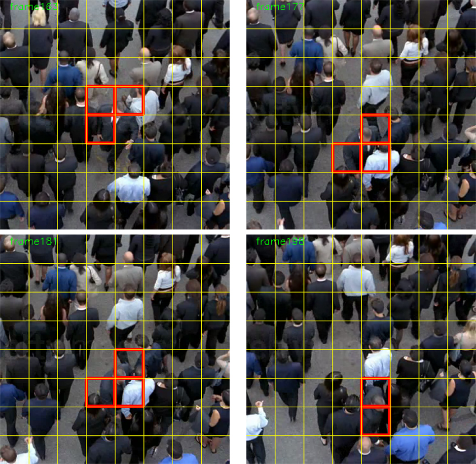
Figure 10. Results obtained by our method (single grid version) on the Wrong Way video at four time points. Blocks including anomalous motion detected by our method are framed in red.

5.4.2. Music Festival Video

In this video sequence, people are starting a “circle pit” during a music festival. The processed video clip contains 18 frames. We took the top half of the first 5 frames to populate the reference LAF histogram space. Sample results are reported in Figure 11. Our algorithm is able to capture the beginning of the anomalous event (Figure 11 left) and correctly delineate it when the circle pit is fully formed (Figure 11 right).

FIGURE 11

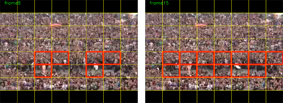
Figure 11. Result samples of the Music Festival video. Blocks including anomalous motion detected by our method (single grid version) are framed in red.

5.5. Drawbacks of Our Method

In previous sections, we described our method and demonstrated its relevance for the complex task of detecting motion-based anomalies in videos. However, our method is not free of drawbacks and failure cases. In particular, since the LOF measure is density-based, a sufficient number of “normal” events should be captured on the training phase of our method. Furthermore, the resolution of detected anomalies is directly related with the chosen block size, together with the capabilities of the chosen motion detector. In other words, anomalies that are too small to be captured by either our block-based method or motion detector might be ignored. Nonetheless, our method provides promising results on real (noisy) datasets, where in fact these issues did not seem to be of major concern. Let us recall that UMN, UCSD, and PETS datasets were built from real commercial surveillance cameras, at low resolutions and with compression artifacts.

5.6. Computation Time

The current implementation of our whole workflow in C++ enables us to process 1.3 frames per second with 2.5 GHz CPU, as reported in Table 7, the computation of the collection of affine motion models included. Several steps of the method are parallelizable, which, if implemented, could lead to greatly decrease the computing time. In particular, computation of per-block histograms and evaluation of LOF, which currently takes around 65% of the total execution time, can be effectively processed in parallel.

TABLE 7

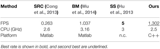
Table 7. Frames per second (FPS) processing of various methods.

We also provide in Table 7 a comparison of the execution time measured in processed frames per second (FPS) for several motion-based anomaly detection methods. We acknowledge that the numbers correspond to different implementations, so that this comparison is only indicative. Besides, the reported execution time may not encompass the whole workflow and the size of the processed images may vary, making computation time comparison tricky. For instance, the execution time for the SS method (Hu et al., 2013) does not include the computation of the optical flow fields and of the cumulative flow word histograms. Nevertheless, our method is prone to process more efficiently than other reported methods, due to its capacity to be highly parallelized.

5.7. Impact of LAF Histograms

In this section, we aim to demonstrate the contribution of the LAF histograms we have introduced. To this end, we compare our algorithm with a modified version of itself. The modification consists in building histograms of optical flow (which translates into histograms of Translation motion classes). In fact, we used optical flows provided by three methods: the pyramidal implementation of the Lucas–Kanade method (LK) (Bouguet, 2001), the variational method defined by Brox et al. (2004), and the polynomial expansion-based flow estimation method (FB) (Farnebäck, 2003). We built these flow-based variants of our method by computing optical flow histograms (HOF) still weighted by motion vector magnitudes (which is equivalent to histograms of Translation classes only), but with more quantized orientations (12 bins). Results on the UCSD ped1 (full ground truth) dataset are reported in Figure 12. They show that our original method greatly outperforms the flow-based versions, which yet benefit from a finer quantization of translation orientations. Our method clearly leverages labeled affine flows and LAF histograms to get superior performance. We believe that the reason is twofold: (i) computing affine flow yields less noisy flow vectors and (ii) introducing histograms of local motion classes bring more explicit information on the nature of the motion.

FIGURE 12

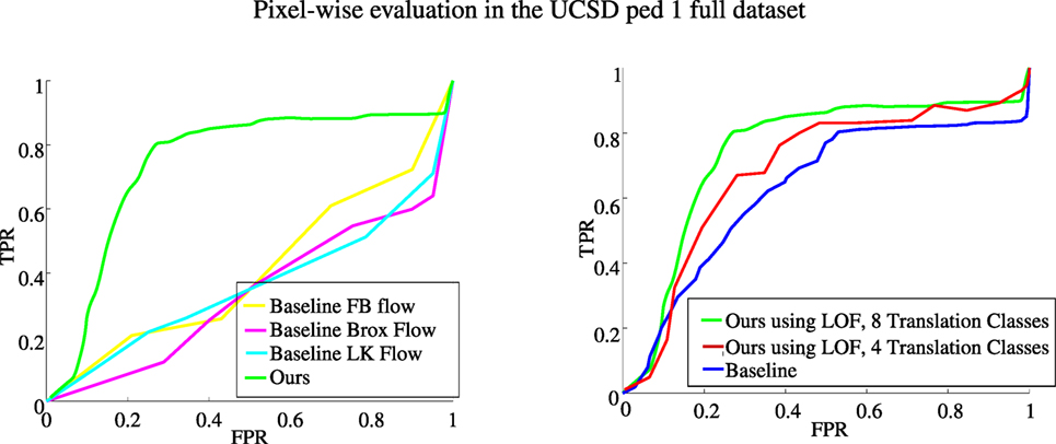
Figure 12. Left: anomaly detection evaluated with the pixel-level criterion. Plots of ROC curves for our method with LAF histograms and for flow-based baselines on the UCSD ped1 (full ground truth) dataset. Right: ROC curves for the pixel-level criterion on the UCSD ped1 dataset with full ground truth. In green: results obtained using the LOF measure and 8 Translation classes. In red: results obtained with the LOF measure with only 4 Translation classes. In blue: results obtained with the baseline version without LOF (histogram distance thresholding).

5.8. Impact of LOF Criterion and Number of Translation Classes

We now demonstrate the beneficial role of the LOF criterion. To assess it, we have compared the LOF criterion to a baseline version of our algorithm which directly thresholds LAF histogram distances. For this baseline version, the histogram $h_i^{\beta }$ extracted from training data is called the “reference histogram” of a given block ${\mathcal{B}}_i$. Each bin l of this histogram is computed as follows:

$h_i^{\beta }\left(l\right)=\frac{1}{T_i}{\displaystyle \sum _{\varsigma =1}^{T_i}}{\displaystyle \sum _{\tau =\varsigma -1}^{\varsigma +1}}{\displaystyle \sum _{p\in {ℬ}_i}}\psi \left(p,\mathrm{\tau },l\right),$ (14)

where T_i is the number of histograms computed over the training sequence corresponding to normal behaviors for block ${\mathcal{B}}_i$, and ψ(p, t, l) is defined in equation (6). In the proposed method described in the paper, these T_i histograms form the feature space where the LOF measure of the histogram $h_i^t$ is computed for a given block ${\mathcal{B}}_i$ at time t. For the baseline method, we compute the average histogram $h_i^{\beta }$ from these T_i histograms as defined in equation (14).

The rule for setting the detection threshold in the baseline version is similar to the one used in our proposed method with LOF but applies directly to the distance between the test histogram $h_i^t$, computed at time instant t, and the reference histogram $h_i^{\beta }$ for the corresponding block ${\mathcal{B}}_i$. The threshold in the baseline version is computed at every block from a p-value on the distribution of distances of the reference histogram to the available training histograms for that block. The same spatiotemporal filtering is applied to the output of the thresholding of the distance between the test histogram and the reference histogram.

We compare these two versions by providing ROC curves obtained on the UCSD ped1 dataset for the pixel-level evaluation criterion in Figure 12. At the same time, we provide results with a smaller number of translation classes for our full LOF-based method. The areas under the ROC curves are summarized in Table 8. With these experiments, it is clearly demonstrated that the local outlier factor is effectively of great importance in our proposed pipeline. Moreover, the use of eight translation classes shows a substantial advantage over using only four translation classes.

TABLE 8

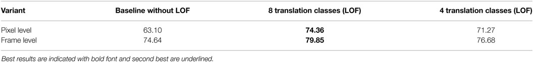
Table 8. Areas under the curves (AUC) of three versions of our anomalous motion detection method on the UCSD ped1 dataset with full ground truth.

5.9. Statistical Significance of the Presented Experiments

In order to determine whether the gain in performance is statistically significant, we adopt a binomial test of statistic significance for all the comparisons at the frame level provided in the previous subsections. The choice of the binomial test is explained by the fact that frame-level detection involves a binary labeling process (normal vs. anomalies). Assuming that the null hypothesis is to have methods with equal score (p₁ = p₂), and the alternative hypothesis to have different scores (p₁ ≠ p₂), we need to compute the test statistic, which is given by

$z=\frac{{\widehat{p}}_1-{\widehat{p}}_2}{\sqrt{\widehat{p}\left(1-\widehat{p}\right)\left(2∕N\right)}},$ (15)

where $\widehat{p}=\frac{{\widehat{p}}_1+{\widehat{p}}_2}{2}$, ${\widehat{p}}_1$, and ${\widehat{p}}_2$ are the computed scores normalized to 0–1 range, and N is the number of frames of the particular experiment (i.e., total number of frames in the videos of the given dataset).

The test is intended to verify if our scores are different (better or worse) to the scores of other methods with a particular degree of statistical significance. We set the test to be at the 95% confidence level. In other words, to reject the null hypothesis, we need to compare z to the critical region value of z_α/2, with the cutoff α = 0.05, i.e., z_α/2 = 1.96. If |z| < z_α/2, the null hypothesis is rejected. We can infer the best method by the sign of z, or, alternatively, the sign of ${\widehat{p}}_1-{\widehat{p}}_2$.

In particular, for the UMN and UCSD dataset we take accuracy scores at the Equal Error Rate point of the ROC curve to evaluate significance. For PETS 2009, we simply use the accuracy scores provided in the “Overall” row of Table 4. All the significance tests are summarized in Table 9.

TABLE 9

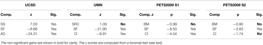
Table 9. Significance of the frame-level experiments for all the presented datasets.

For UMN, it turns out that SRC and our method are not statistically different, but our method surpasses with statistical significance SF and CI methods. Similarly, for the PETS 2009 experiments, the results of our method are significantly better than FF, CI and SF methods. Our improvement over BM turned out to be not significant under the 95% confidence test. Finally, for UCSD dataset, all the results from Table 5 are statistically significant when comparing our multi-grid method against all the others (including our single-grid method).

6. Conclusion

We have presented an original and efficient anomalous motion detection-and-localization method which can capture diverse kinds of anomalous motion in common real scenarios. It can work in a fully unsupervised and online way for crowded scenes. The LAF histogram and the data-driven detection criterion based on the LOF factor are two distinctive contributions of our approach. Threshold value for anomaly detection decision can be automatically and locally adapted, based on statistical arguments. The current implementation of our algorithm is fast, although it could be significantly further accelerated by doing massive parallelization over blocks. Our method supplies state-of-the art results in several experiments and competitive results for the other ones. It can successfully deal with datasets comprising different camera viewpoints and dynamic contents involving both local and global anomalous motion. Local anomalous motion localization is inherent in the block-based proposed method and was experimentally demonstrated accurate enough.

Author Contributions

The authors equally contribute to the research and the paper writing.

Conflict of Interest Statement

The authors declare that the research was conducted in the absence of any commercial or financial relationships that could be construed as a potential conflict of interest.

Acknowledgments

We thank the authors of Antic and Ommer (2011) and Cong et al. (2013) for providing us useful experimental data. We would also like to thank the authors of Ferryman and Shahrokni (2009), Li et al. (2014), and Papanikolopoulos (2005) for generating the datasets that were used in the experimental section of this paper, and for providing them to the public for use and reproduction without need of any permissions. This work was partially supported by Région Bretagne (Brittany Council) through a contribution to AB’s PhD student grant.

Footnote

1. ^http://www.irisa.fr/vista/Motion2D/.

References

Adam, A., Rivlin, E., Shimshoni, I., and Reinitz, D. (2008). Robust real-time unusual event detection using multiple fixed-location monitors. IEEE Trans. Pattern Anal. Mach. Intell. 30, 555–560. doi: 10.1109/TPAMI.2007.70825

CrossRef Full Text | Google Scholar

Aggarwal, J. K., and Ryoo, M. S. (2011). Human activity analysis: a review. ACM Comput. Surv. 43, 16. doi:10.1145/1922649.1922653

CrossRef Full Text | Google Scholar

Andersson, M., Gustafsson, F., St-Laurent, L., and Prevost, D. (2013). Recognition of anomalous motion patterns in urban surveillance. IEEE J. Sel. Top. Signal Process. 7, 102–110. doi:10.1109/JSTSP.2013.2237882

CrossRef Full Text | Google Scholar

Antic, B., and Ommer, B. (2011). “Video parsing for abnormality detection,” in ICCV, Barcelona.

Google Scholar

Basharat, A., Gritai, A., and Shah, M. (2008). “Learning object motion patterns for anomaly detection and improved object detection,” in CVPR, Anchorage.

Google Scholar

Basset, A., Bouthemy, P., and Kervrann, C. (2014). “Recovery of motion patterns and dominant paths in videos of crowded scenes,” in ICIP.

Google Scholar

Benezeth, Y., Jodoin, P.-M., and Saligrama, V. (2011). Abnormality detection using low-level co-occurring events. Pattern Recognit. Lett. 32, 423–431. doi:10.1016/j.patrec.2010.10.008

CrossRef Full Text | Google Scholar

Bertini, M., Del Bimbo, A., and Seidenari, L. (2012). Multi-scale and real-time non-parametric approach for anomaly detection and localization. Comput. Vis. Image Underst. 116, 320–329. doi:10.1016/j.cviu.2011.09.009

CrossRef Full Text | Google Scholar

Biswas, S., and Babu, R. V. (2014). “Sparse representation based anomaly detection with enhanced local dictionaries,” in ICIP, Paris.

Google Scholar

Boiman, O., and Irani, M. (2007). Detecting irregularities in images and in video. Int. J. Comput. Vis. 74, 17–31. doi:10.1007/s11263-006-0009-9

CrossRef Full Text | Google Scholar

Bouguet, J.-Y. (2001). Pyramidal Implementation of the Affine Lucas Kanade Feature Tracker. Description of the Algorithm. Standford: Intel Co, 5.

Google Scholar

Breunig, M. M., Kriegel, H.-P., Ng, R. T., and Sander, J. (2000). “LOF: identifying density-based local outliers,” in ACM SIGMOD Record, Vol. 29, 93–104.

Google Scholar

Brox, T., Bruhn, A., Papenberg, N., and Weickert, J. (2004). “High accuracy optical flow estimation based on a theory for warping,” in ECCV, Prague.

Google Scholar

Cavanaugh, J. E. (1997). Unifying the derivations for the Akaike and corrected Akaike information criteria. Stat. Probab. Lett. 33, 201–208. doi:10.1016/S0167-7152(96)00128-9

CrossRef Full Text | Google Scholar

Cedras, C., and Shah, M. (1995). Motion-based recognition a survey. Image Vis. Comput. 13, 129–155. doi:10.1016/0262-8856(95)93154-K

CrossRef Full Text | Google Scholar

Cha, S.-H., and Srihari, S. N. (2002). On measuring the distance between histograms. Pattern Recognit. 35, 1355–1370. doi:10.1016/S0031-3203(01)00118-2

CrossRef Full Text | Google Scholar

Chandola, V., Banerjee, A., and Kumar, V. (2009). “Anomaly detection: a survey,” in ACM CSUR (New York), 41.

Google Scholar

Chen, D.-Y., and Huang, P.-C. (2011). Motion-based unusual event detection in human crowds. J. Vis. Commun. Image Represent. 22, 178–186. doi:10.1016/j.jvcir.2010.12.004

CrossRef Full Text | Google Scholar

Cheng, K.-W., Chen, Y.-T., and Fang, W.-H. (2015). “Video anomaly detection and localization using hierarchical feature representation and Gaussian process regression,” in CVPR, Boston.

Google Scholar

Chockalingam, T., Emonet, R., and Odobez, J.-M. (2013). “Localized anomaly detection via hierarchical integrated activity discovery,” in AVSS, Krakow.

Google Scholar

Cong, Y., Yuan, J., and Liu, J. (2013). Abnormal event detection in crowded scenes using sparse representation. Pattern Recognit. 46, 1851–1864. doi:10.1016/j.patcog.2012.11.021

CrossRef Full Text | Google Scholar

Crivelli, T., Bouthemy, P., Cernuschi-Frias, B., and Yao, J.-F. (2011). Simultaneous motion detection and background reconstruction with a conditional mixed-state Markov random field. Int. J. Comput. Vis. 94, 295–316. doi:10.1007/s11263-011-0429-z

CrossRef Full Text | Google Scholar

Cui, X., Liu, Q., Gao, M., and Metaxas, D. N. (2011). “Abnormal detection using interaction energy potentials,” in CVPR, Colorado Springs.

Google Scholar

Fang, Y., Wang, Z., Lin, W., and Fang, Z. (2014). Video saliency incorporating spatiotemporal cues and uncertainty weighting. IEEE Trans. Image Process. 23, 3910–3921. doi:10.1109/TIP.2014.2336549

PubMed Abstract | CrossRef Full Text | Google Scholar

Farnebäck, G. (2003). “Two-frame motion estimation based on polynomial expansion,” in SCIA, Halmstad.

Google Scholar

Ferryman, J., and Shahrokni, A. (2009). “An overview of the PETS 2009 challenge,” in PETS.

Google Scholar

Fortun, D., Bouthemy, P., and Kervrann, C. (2015). Optical flow modeling and computation: a survey. Comput. Vis. Image Underst. 134, 1–21. doi:10.1016/j.cviu.2015.02.008

CrossRef Full Text | Google Scholar

Georgiadis, G., Ayvaci, A., and Soatto, S. (2012). “Actionable saliency detection: Independent motion detection without independent motion estimation,” in CVPR, Rhode Island.

Google Scholar

Goyette, N., Jodoin, P.-M., Porikli, F., Konrad, J., and Ishwar, P. (2014). A novel video dataset for change detection benchmarking. IEEE Trans. Image Process. 23, 4663–4679. doi:10.1109/TIP.2014.2346013

PubMed Abstract | CrossRef Full Text | Google Scholar

Hospedales, T., Gong, S., and Xiang, T. (2012). Video behaviour mining using a dynamic topic model. Int. J. Comput. Vis. 98, 303–323. doi:10.1007/s11263-011-0510-7

CrossRef Full Text | Google Scholar

Hu, Y., Zhang, Y., and Davis, L. (2013). “Unsupervised abnormal crowd activity detection using semiparametric scan statistic,” in CVPRW, Portland.

Google Scholar

Huang, C.-R., Chang, Y.-J., Yang, Z.-X., and Lin, Y.-Y. (2014). Video saliency map detection by dominant camera motion removal. IEEE Trans. Circuits Syst. Video Technol. 24, 1336–1349. doi:10.1109/TCSVT.2014.2308652

CrossRef Full Text | Google Scholar

Huber, P. J. (1981). Robust Statistics. New Jersey: Wiley.

Google Scholar

Itti, L., and Baldi, P. (2005). “A principled approach to detecting surprising events in video,” in CVPR, San Diego.

Google Scholar

Jiang, F., Yuan, J., Tsaftaris, S. A., and Katsaggelos, A. K. (2011). Anomalous video event detection using spatiotemporal context. Comput. Vis. Image Underst. 115, 323–333. doi:10.1016/j.cviu.2010.10.008

CrossRef Full Text | Google Scholar

Jiang, M., Xu, J., and Zhao, Q. (2014). “Saliency in crowd,” in ECCV, Zurich.

Google Scholar

Kim, J., and Grauman, K. (2009). “Observe locally, infer globally: a space-time mrf for detecting abnormal activities with incremental updates,” in CVPR, Miami Beach.

Google Scholar

Kim, W., and Kim, C. (2014). Spatiotemporal saliency detection using textural contrast and its applications. IEEE Trans. Circuits Syst. Video Technol. 24, 646–659. doi:10.1109/TCSVT.2013.2290579

CrossRef Full Text | Google Scholar

Kratz, L., and Nishino, K. (2009). “Anomaly detection in extremely crowded scenes using spatio-temporal motion pattern models,” in CVPR, Miami Beach.

Google Scholar

Lazarevic, A., Ertöz, L., Kumar, V., Ozgur, A., and Srivastava, J. (2003). “A comparative study of anomaly detection schemes in network intrusion detection,” in SIAM Data Mining, San Francisco.

Google Scholar

Leach, M. J., Sparks, E. P., and Robertson, N. M. (2014). Contextual anomaly detection in crowded surveillance scenes. Pattern Recognit. Lett. 44, 71–79. doi:10.1016/j.patrec.2013.11.018

CrossRef Full Text | Google Scholar

Lee, D.-G., Suk, H.-I., Park, S.-K., and Lee, S.-W. (2015). Motion influence map for unusual human activity detection and localization in crowded scenes. IEEE Trans. Circuits Syst. Video Technol. 25, 1612–1623. doi:10.1109/TCSVT.2015.2395752

CrossRef Full Text | Google Scholar

Li, C., Han, Z., Ye, Q., and Jiao, J. (2013). Visual abnormal behavior detection based on trajectory sparse reconstruction analysis. Neurocomputing 119, 94–100. doi:10.1016/j.neucom.2012.03.040

CrossRef Full Text | Google Scholar

Li, J., Liu, Z., Zhang, X., Le Meur, O., and Shen, L. (2015a). Spatiotemporal saliency detection based on superpixel-level trajectory. Signal Process. Image Commun. 38, 100–114. doi:10.1016/j.image.2015.04.014

CrossRef Full Text | Google Scholar

Li, T., Chang, H., Wang, M., Ni, B., Hong, R., and Yan, S. (2015b). Crowded scene analysis: a survey. IEEE Trans. Circuits Syst. Video Technol. 25, 367–386. doi:10.1109/TCSVT.2014.2358029

CrossRef Full Text | Google Scholar

Li, W., Mahadevan, V., and Vasconcelos, N. (2014). Anomaly detection and localization in crowded scenes. IEEE Trans. Pattern Anal. Mach. Intell. 36, 18–32. doi:10.1109/TPAMI.2013.111

PubMed Abstract | CrossRef Full Text | Google Scholar

Lu, C., Shi, J., and Jia, J. (2013). “Abnormal event detection at 150 fps in Matlab,” in ICCV, Sydney.

Google Scholar

Mahadevan, V., Li, W., Bhalodia, V., and Vasconcelos, N. (2010). “Anomaly detection in crowded scenes,” in CVPR, San Francisco.

Google Scholar

Mahadevan, V., and Vasconcelos, N. (2010). Spatiotemporal saliency in dynamic scenes. IEEE Trans. Pattern Anal. Mach. Intell. 32, 171–177. doi:10.1109/TPAMI.2009.112

PubMed Abstract | CrossRef Full Text | Google Scholar

Mehran, R., Oyama, A., and Shah, M. (2009). “Abnormal crowd behavior detection using social force model,” in CVPR, Miami Beach.

Google Scholar

Mo, X., Monga, V., Bala, R., and Fan, Z. (2014). Adaptive sparse representations for video anomaly detection. IEEE Trans. Circuits Syst. Video Technol. 24, 631–645. doi:10.1109/TCSVT.2013.2280061

CrossRef Full Text | Google Scholar

Odobez, J.-M., and Bouthemy, P. (1995). “Robust multiresolution estimation of parametric motion models,” in JVCIR (Amsterdam), Vol. 6, 348–365.

Google Scholar

Papanikolopoulos, N. (2005). Unusual Crowd Behaviour Dataset. University of Minnesota. Available at: http://mha.cs.umn.edu/Movies/Crowd-Activity-All.avi

Google Scholar

Pécot, T., Bouthemy, P., Boulanger, J., Chessel, A., Bardin, S., Salamero, J., et al. (2015). Background fluorescence estimation and vesicle segmentation in live cell imaging with conditional random fields. IEEE Trans. Image Process. 24, 667–680. doi:10.1109/TIP.2014.2380178

PubMed Abstract | CrossRef Full Text | Google Scholar

Piciarelli, C., Micheloni, C., and Foresti, G. L. (2008). Trajectory-based anomalous event detection. IEEE Trans. Circuits Syst. Video Technol. 18, 1544–1554. doi:10.1109/TCSVT.2008.2005599

CrossRef Full Text | Google Scholar

Porikli, F., and Haga, T. (2004). “Event detection by eigenvector decomposition using object and frame features,” in CVPRW, Washington.

Google Scholar

Roshtkhari, M. J., and Levine, M. D. (2013). An on-line, real-time learning method for detecting anomalies in videos using spatio-temporal compositions. Comput. Vis. Image Underst. 117, 1436–1452. doi:10.1016/j.cviu.2013.06.007

CrossRef Full Text | Google Scholar

Solmaz, B., Moore, B. E., and Shah, M. (2012). Identifying behaviors in crowd scenes using stability analysis for dynamical systems. IEEE Trans. Pattern Anal. Mach. Intell. 34, 2064–2070. doi:10.1109/TPAMI.2012.123

PubMed Abstract | CrossRef Full Text | Google Scholar

Stauffer, C., and Grimson, W. E. L. (2000). Learning patterns of activity using real-time tracking. IEEE Trans. Pattern Anal. Mach. Intell. 22, 747–757. doi:10.1109/34.868677

CrossRef Full Text | Google Scholar

Thida, M., Yong, Y. L., Climent-Pérez, P., Eng, H.-L., and Remagnino, P. (2013). “A literature review on video analytics of crowded scenes,” in IMS (Berlin Heidelberg: Springer), 17–36.

Google Scholar

Varadarajan, J., Emonet, R., and Odobez, J.-M. (2007). A sequential topic model for mining recurrent activities from long term video logs. Int. J. Comput. Vis. 103, 100–126. doi:10.1007/s11263-012-0596-6

CrossRef Full Text | Google Scholar

Veit, T., Cao, F., and Bouthemy, P. (2011). An a contrario decision framework for region-based motion detection. Int. J. Comput. Vis. 68, 163–178. doi:10.1007/s11263-006-6661-2

CrossRef Full Text | Google Scholar

Vishwakarma, S., and Agrawal, A. (2013). A survey on activity recognition and behavior understanding in video surveillance. Vis. Comput. 29, 983–1009. doi:10.1007/s00371-012-0752-6

CrossRef Full Text | Google Scholar

Wang, W., Shen, J., and Shao, L. (2015). Consistent video saliency using local gradient flow optimization and global refinement. IEEE Trans. Image Process. 24, 4185–4196. doi:10.1109/TIP.2015.2460013

PubMed Abstract | CrossRef Full Text | Google Scholar

Wang, X., Ma, K. T., Ng, G.-W., and Grimson, W. E. L. (2011). Trajectory analysis and semantic region modeling using nonparametric hierarchical Bayesian models. Int. J. Comput. Vis. 95, 287–312. doi:10.1007/s11263-011-0459-6

CrossRef Full Text | Google Scholar

Wang, X., Ma, X., and Grimson, W. E. L. (2009). Unsupervised activity perception in crowded and complicated scenes using hierarchical Bayesian models. IEEE Trans. Pattern Anal. Mach. Intell. 31, 539–555. doi:10.1109/TPAMI.2008.87

PubMed Abstract | CrossRef Full Text | Google Scholar

Wu, S., Moore, B. E., and Shah, M. (2010). “Chaotic invariants of Lagrangian particle trajectories for anomaly detection in crowded scenes,” in CVPR, San Francisco.

Google Scholar

Wu, S., Wong, H.-S., and Yu, Z. (2014). A Bayesian model for crowd escape behavior detection. IEEE Trans. Circuits Syst. Video Technol. 24, 85–98. doi:10.1109/TCSVT.2013.2276151

CrossRef Full Text | Google Scholar

Zen, G., Ricci, E., and Sebe, N. (2012). “Exploiting sparse representations for robust analysis of noisy complex video scenes,” in ECCV, Firenze.

Google Scholar

Zhan, B., Monekosso, D. N., Remagnino, P., Velastin, S. A., and Xu, L.-Q. (2008). Crowd analysis: a survey. Mach. Vis. Appl. 19, 345–357. doi:10.1007/s00138-008-0132-4

CrossRef Full Text | Google Scholar

Zhang, D., and Lu, G. (2001). Segmentation of moving objects in image sequence: a review. IEEE Trans. Circuits Syst. Signal Process. 20, 143–183. doi:10.1007/BF01201137

CrossRef Full Text | Google Scholar

Zhang, Y., Lu, H., Zhang, L., and Ruan, X. (2016). Combining motion and appearance cues for anomaly detection. Pattern Recognit. 51, 443–452. doi:10.1016/j.patcog.2015.09.005

CrossRef Full Text | Google Scholar

Zhang, Y., Qin, L., Ji, R., Yao, H., and Huang, Q. (2015). Social attribute-aware force model: exploiting richness of interaction for abnormal crowd detection. IEEE Trans. Circuits Syst. Video Technol. 25, 1231–1245. doi:10.1109/TCSVT.2014.2355711

CrossRef Full Text | Google Scholar

Zhao, B., Fei-Fei, L., and Xing, E. P. (2011). “Online detection of unusual events in videos via dynamic sparse coding,” in CVPR, Colorado Springs.

Google Scholar

Zhong, H., Shi, J., and Visontai, M. (2004). “Detecting unusual activity in video,” in CVPR, Washington.

Google Scholar

Zhu, X., Liu, J., Wang, J., Li, C., and Lu, H. (2014). Sparse representation for robust abnormality detection in crowded scenes. Pattern Recognit. 47, 1791–1799. doi:10.1016/j.patcog.2013.11.018

CrossRef Full Text | Google Scholar