Using Spatial Reinforcement Learning to Build Forest Wildfire Dynamics Models From Satellite Images

1. Introduction

There is a clear and growing need for advanced analytical and decision-making tools as demands for sustainable management increase and as the consequences of inadequate resources for decision-making become more profound. Artificial intelligence and machine learning methods provide ways to combine multiple modes of information such as spatial statistical ground data, weather data, and satellite imagery into a unified model for classification or prediction.

One high impact example of this potential is forest wildfire management. The risk, costs, and impacts of forest wildfires are a perennial and unavoidable concern in many parts of the world. A number of factors contribute to the increasing importance and difficulty of this domain in future years including climate change, growing urban sprawl into areas of high wildfire risk, and past fire management practices which focused on immediate suppression at the cost of increased future fire risk (Montgomery, 2014).

There are a wide range of challenging decision and optimization problems in the area of forest fire management (Martell, 2015), many of which would benefit from more responsive fire behavior models which could be run quickly and updated easily based on new data. For example, one simple decision problem is whether to allow a fire to burn or not, since burning is a natural form of fuel reduction treatment. Answering this question requires a great deal of expensive simulations to evaluate the policy options fully (Houtman et al., 2013).

These simulations are built by an active research community for forest and wildland fire behavior modeling. Data are collected using trials in real forest conditions, controlled lab burning experiments, physics-based fire modeling, and more (Finney et al., 2013). These hand crafted physics-based models’ simulations have high accuracy but are expensive to create and update and computationally expensive to use. The question we ask is: Can we learn a dynamics model from readily available satellite image data and treating wildfire as an agent spreading across a landscape in response to neighborhood environmental and landscape parameters?

In this work, we provide evidence for an affirmative answer to this question by introducing a new approach for using reinforcement learning (RL) (Sutton and Barto, 1998) to automatically learn wildfire spread dynamics models by treating fire as an agent on the landscape taking spatial actions in reaction to its environment (Subramanian and Crowley, 2017).

Forest wildfire spread as a specific case of a more general problem which we call spatially spreading processes (SSPs), which occur when local features are changed over time by some dynamic process which is a function of properties at different locations in space and their proximity to the target location. This is to be distinguished from mere prediction of impact of a physical object moving across space as the SSP can be active in many, or all, locations at once. This is also more than merely spatial auto-correlation that measures the degree to which features at two locations are similar based on their proximity. Spatial auto-correlation can be an indicator of the presence of an SSP, but the dynamic changes over time between spatial locations may not result in values being similar or inversely correlated in a simple way. In many of these domains, the dynamics are often modeled by hand using agent-based models and geostatistics methods. In other areas, they are increasingly learned from data streams by being treated as videos. However, each of these approaches has their drawbacks. One of the goals of our research is to find novel representations of local dynamics for SSPs that can provide transparent and interpretative solutions to learning of dynamics models and decision-making across many domains. The approach proposed here offers the tantalizing possibility to represent and learn a causal agent-based policy representation using RL which would be a much easier model to interpret and analyze for human decision makers.

In this article, we carry out experiments on the accuracy of interpolation and forward prediction using five different RL algorithms in a new formulation of agent-based learning. We use easily accessible Landsat satellite data from the USGS satellite data portal and provide a prediction accuracy of resulting policies learned with each algorithm upon comparison with the same. The dataset is a set of satellite photos of massive wild fires in Northern Alberta in 2011 and 2016. We show that Monte Carlo Tree search and the Deep RL algorithm A3C (Mnih et al., 2013) perform the best but have advantages in different situations in this domain. For comparison, we also implemented a Gaussian Process (GP) classifier (Rasmussen and Williams, 2006) as a supervised learning model on the dataset. This classifier places a Gaussian Process prior on a latent function, which is then squashed to the domain [0, 1] through a link function to obtain the probabilistic classification.

This approach has applications in forest wildfire management and opens up possibilities for interpretative dynamics models as well as providing new challenging data sets for RL research. Our approach promises to provide another source of validation for existing wildfire models as well as gives us the opportunity to perform faster and more accurate prediction by learning patterns in the raw data. Another application of our approach would be learning transferable models from one data-rich region or time period and applying it to another region or time period where less data are available if there is evidence that fires in both regions behave similarly.

In prior work (Houtman et al., 2013), we have used standard, physics-based simulators such as Farsite (Finney, 1998) to carry out automated planning of fire control policies using Monte Carlo simulations and optimization. These simulations took on the order of 1 h to run for 100-year simulations of forest fire futures, which present a challenge when thousands of simulation trajectories are needed for statistical confidence. Thus, augmenting these detailed simulators with faster approximations learned from data could improve the ability to do automated planning.

2. Review of Literature

We provide an overview of the relevant literature on the forest wildfire prediction and management problem in general and then on the previous use of machine learning algorithms for this domain.

2.1. Machine Learning on Satellite Imagery

Researchers have attempted to use machine learning in combination with satellite imagery in a series of ecological applications in the past. In Kubat et al. (1998), the authors use satellite radar images and machine learning for the detection of oil spills. Algorithms, such as C4.5 and 1-nearest neighbor, are used along with expert rules to train the classifier which the authors specify was hard and not completely accurate. Our work completely removes the need for such expert rules.

In Jean et al. (2016), satellite imagery and machine learning has been used to tackle the case of poverty. Convolutional neural nets and transfer learning have been used to derive models having good performances in terms of accuracy. This research demonstrated how machine learning tools, which are typically suited for data-rich domains, can be used for data-scarce settings too.

Coral reef research is another aspect that has been studied using satellite images and machine learning (Knudby et al., 2010). In Knudby et al. (2010), a series of statistical and machine learning models have been used on the IKONOS satellite imagery to produce spatially explicit predictions of species richness, biomass, and diversity of fish community. This research motivates the exploration of importance of different variables in the predictive models by using permutations techniques.

2.2. Forest Wildfire Prediction and Management

Montgomery (2014) discusses the increased future fire risk at the consequence of fire management practices, which focused on immediate suppression. The three core themes of externalities, incentives, and risk-based decision analysis in the case of wild fire suppression are described. The goal is to determine how the core themes contribute to the evolution of an effective future fire policy. This problem is also enumerated in Houtman et al. (2013).

The standard for wildland fire behavior and forest fire modeling is described in Finney et al. (2013), which carried out exhaustive lab experiments, real forest condition simulations, and trials to build sound and coherent fire spread theory for model reliability. The resulting models are used by the US Forest Service but are very computationally expensive to run. The model accuracy also varies widely across wild fires in different regions. Cellular automaton models are also widely used to predict wildfire spread (Yongzhong et al., 2004). Our approach is easier to apply than these methods and is shown to perform better than the same.

The work in Martell (2015) describes the need for a computationally simple and accurate model for wild fires. They highlight a number of challenging decision and optimization problems in the area of forest fire management and recent efforts to develop decision support tools to overcome them. The focus is on using methods of Operations Research to aid fire managers making complex decisions about fire suppression and resource allocation.

2.3. Machine Learning in Forest Fire Management

In Castelli et al. (2015), the authors discuss the application of an intelligent system based on genetic programming for the prediction of burned areas in a wild fire situation. They also compare the genetic programming methodology to state-of-the-art machine learning techniques in fire modeling and conclude that genetic programming techniques are better. The major machine learning techniques used are SVM with a polynomial kernel, random forests, radial basis function network, linear regression, isotonic regression, and neural networks.

Significant problems have arisen while dealing with large databases or long periods of observation (e.g., pattern recognition, geophysical monitoring, monitoring of rare events (natural hazards), etc.). The authors in Forsell et al. (2009) stipulate that the major problems in such cases are how to explore, analyze, and visualize the oceans of available information. Several important applications of machine learning algorithms for geospatial data are presented: regional classification of environmental data, mapping of continuous environmental data including automatic algorithms and optimization (design/redesign) of monitoring networks.

Machine learning algorithms use an automatic inductive approach to recognize patterns in data. Once learned, pattern relationships are applied to other similar data to generate predictions for data-driven classification and regression problems. The work in Cracknell and Reading (2014) takes a task of supervised lithology classification (geological mapping) using airborne images and multispectral satellite data and compares the application of popular machine learning techniques to the same. A 10-fold cross validation was used to select the optimal parameters to be used in all the methods. These selected parameters were used to train the machine Learning classification models on the entire set of samples.

In Sehgal et al. (2006), the authors use a machine learning approach for Geospatial Entity resolution which is the problem of consolidating data from diverse sources into a single data source referenced by location (in the form of coordinates). Several feature-based matching techniques like location name matching, coordinate matching, and location-type matching are introduced and evaluated. These feature-based matching techniques use each location feature independently. A new method integrating spatial and non-spatial features and learning a combined spatial similarity measure is introduced.

Modeling forest areas is concentrated upon in Garzón et al. (2006). The environmental variables consisting of both topographic and climatic factors are considered in this work. A modeling framework for habitat modeling is established to train, test, and validate the popular predictive machine learning methods. Neural Networks, Random Forests, and Tree-Based Classification are used as predictive models. A ROC curve (Specificity vs Sensitivity graph) analysis is done for parameter selection. Species distribution and habitat modeling are described to be complex problems much like the wild fire problem with many responsible factors and the authors admit that modeling all the factors are impossible with the current state of the art. Hence, having an agent-based approach that learns the relevant factors on its own seems to be the most suitable idea.

Machine learning is used for the spatial interpolation of environmental variables in Li et al. (2011). In this study, around 23 methods are considered including popular machine learning methods and their combinations. Along with machine learning, the considered methods were drawn from a large pool of categories including geostatistical methods, non geostatistical methods, statistical methods, and combined methods. The dataset consists of about 177 samples of sea bed mud content in the southwest of Australian Exclusive Economic Zone, and the problem is to determine the mud content in the other points by interpolation. Several primary and secondary variables are considered to influence this decision. Random forest seems to perform the best among the methods considered. RF performance was attributed to its relative robustness to outliers and noise, its nature of not over fitting with respect to the source data, and its ability to model complex interactions.

Recknagel (2001) discusses a summary of all the different ecological modeling applications of machine learning. Artificial Neural nets, Genetic Algorithm methods, and Adaptive Agents seem to perform the best, but they seem to have advantages for different problems. The conclusions are that Artificial Neural Nets perform well in problems of non-linear ordination, visualization, multiple regression, time series modeling, and image recognition and classification. Genetic algorithms are suitable to evolve causal rules, process equations, and optimize process parameters. Adaptive agents are suggested for providing a novel framework in the aid of the discovery and forecasting of emergent ecosystem structures and behaviors in response to environmental changes. This review demonstrates that while various classical AI and ML techniques have been applied to this domain in preliminary forms, there is a gap in the literature on attempting to use modern deep learning and RL techniques.

The existing state-of-the-art methods for building fire prediction models directly satellite images include the Forest Fire risk prediction model used in China (Zhang et al., 2011), the Canadian systems like Forest Fire Weather Index (FWI) System, and the Forest Fire Behavior Prediction (FBP) System (Stocks et al., 1989; Zhang et al., 2011). These systems are still quite difficult to implement due to the requirement of large amount of heterogeneous sources of data such as fuel property and fire characteristics (Zhang et al., 2011), which requires data from high resolution close-range sensors. The work by Alkhatib (2014) explains the advantages of the satellite-based fire prediction systems but specifies that the temporal resolution of available data serves as a serious impediment. Our work specifies a method to learn from available data and reliably interpolate to fill the missing spaces to get an acceptable overall performance.

We model the forest fire domain as a Markov Decision Process (MDP). This approach is becoming more common (Mcgregor et al., 2016), but these are usually focused on finding treatment actions to be taken to reduce or alter fire spread. We take the novel approach of modeling the fire itself as a decision agent attempting to minimize prediction error. This is related to work in Forsell et al. (2009), which investigated using the state variable to represent land vegetation cover and environmental characteristics but to use the action variable to represent interaction between characteristics of nearby locations. This was not on a domain as dynamic as forest fire, however, and our approach differs entirely in implementation.

Machine learning has also been used to detect and classify burn areas in Indian forests (Saranya and Hemalatha, 2012). Saranya and Hemalatha (2012) use spatial data mining to obtain useful information from a series of datasets and subsequently apply supervised algorithms such as Artificial Neural Nets (ANN) and Sequential minimal optimization (SMO) to quantify ignition risk of different regions and hence predict the occurrence of fires. Similarly, Sitanggang and Ismail (2011) use Decision Trees and a series of IF–THEN rules to develop a classification model for forest fires in Indonesia. We prove the superiority of RL techniques to such supervised methods in our work. For instance, the results in Sitanggang and Ismail (2011) show an accuracy of about 63%, whereas our best RL models perform much better than that in similar test cases. In addition, Angayarkkani and Radhakrishnan (2009) use fuzzy logic and fuzzy membership rules to make a forest fire detection system from satellite images. The methods outlined are only capable of predicting fires at the time of satellite image availability, and it is not possible to predict forward or in-between as demonstrated in our work.

Our work also has similarities to the use of intelligent systems for predicting burned areas as suggested in Castelli et al. (2015). However, that work focused on burned area alone whereas we look at the more specific problem of prediction of actual fire spread location over the short term.

3. Problem Formulation

The problem is formulated as a Markov Decision Process (MDP) <S, A, P, R> where the set of states S describes any location on the landscape. A state s ∈ S corresponds to the state of a cell in the landscape (x, y, t, l, w, d, rh, r) where x and y are the location of the cell, t is the temperature at the particular time and location, and l is the land cover type of the cell, which could be one of water, vegetation, built up, bare land, and other (derived from satellite images), and w and d are wind speed and direction, rh is relative humidity, and r is amount of rainfall. The “agent” taking actions is a fire spreading across the landscape. The action a ∈ A indicates the direction the fire at a particular cell “chooses” to move: north, south, east, or west or to stay put. These variables are considered to be the most contributing to fires as they are the primary variables in the Canadian Forest fire weather index as specified in Cortez and Morais (2007).

The dynamics function for any particular cell P(s′|s, a) is a mapping from one state s to the next s′ given an action a. Note, unlike most RL domains where the unknown dynamics of the system can be very complex, in our formulation the dynamics are actually straightforward. Most properties of the cell state do not change quickly, or at all, in response to our actions. So the action of spreading a fire into a neighboring cell directly alters p in that cell, the probability that the neighboring cell in that direction will move to a burn state.

The reward function R maps a cell state to a continuous value in the range [−1, 1]. Rewards are based on the land-cover, for example, a cell predominantly filled with water has less chance catching fire compared with one filled with vegetation. Thus, there is a negative reward for choosing to spread fire to a cell with high percentage of water and a small positive reward for choosing to spread to a cell covered with vegetation. Other reward function components, are derived from the ground truth data for the training sets. Thus, in the training phase, the fire is given a positive reward for taking action choices similar to the actual scenario and negative rewards otherwise. These are applied for particular experiments and algorithms as explained in the experimental setup.

Figure 1 shows a schematic representation of the domain where some cells are currently affected by fire and have a potential to spread fire to other cells nearby which is treated as the “decision” of an agent at that location. The task then is to learn a policy for this agent, which minimizes the total error at different future steps.

FIGURE 1

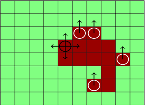
Figure 1. Forest wildfire satellite data domain: a schematic of the wildfire motion domain at a particular state and timestep. The red (dark) cells are on fire, the green cells (light) are not on fire, and the dark circle indicates the current cell or agent being spread by the policy. The arrows around the dark circle indicate the action choices possible. The white circle indicates that other cells will be considered for spread. The arrows from the white circle indicate that there is a strong wind blowing toward north, and the north action is the most likely action choice for these cells (effect of wind).

The initial state will come from satellite images that correspond to the beginning of a fire. We are focusing on fire growth rather than ignition detection, so we set certain cells to have just ignited fire and assign these to the initial state. As it is impossible to predict precisely from where a “fire starts,” these ignited cells are decided based on thermal image data, media reports, and approximations based on the burning areas in the first day on which the satellite image is available. Wind speed and wind direction are assumed to be a constant for a small area at a fixed point of time.

The goal is to learn a policy for this agent that recreates the spread of the fire observed in later satellite images by maximizing discounted rewards designed to reward high accuracy simulation. Actions are constrained to not cross the boundary of the domain of study.

3.1. Data Acquisition

The Richardson fire occurred in a region called Richardson Backcountry north of Fort McMurray in Northern Alberta in 2011. Fort McMurray was also affected by forest fires in 2016 during the massive Fort McMurray fires (Woo and Tait, 2016). The coordinates of Fort McMurray is (56°43′36″ N, 111°22′51″ W) and the coordinates of Richardson Backcountry is (57°22′02.3″ N, 111°19′27.1″ W). The satellite images are downloaded from the USGS Earth Explorer data portal¹ for Alberta. The Landsat Enhanced Thematic Mapper Plus (ETM +) sensor carried on Landsat 7 was the most important source of data. A summary (Kanevski et al., 2008) of the merits of various software packages and tools (such as GeoMISC, GeoKNN, GeoMLP, etc.) in relation to machine learning on geospatial data was useful in developing this work. Figure 2 shows an example where the smoke over burning areas can be seen. A series of visual and thermal images corresponding to the duration of occurrence of the Fort McMurray fire (approximately from April 2016 to September 2016) and Richardson fire (approximately from May 2011 to October 2011) were collected for the corresponding regions of Alberta. All the images were corrected for missing values and outliers. Additional pre-processing steps were carried out as outlined in Cracknell and Reading (2014). These images gave a clear description of the ground scenario in case of fire and are a reliable source of burn areas. The pixels on fire are clearly at a far higher temperature corresponding to the pixels not on fire, and this can be easily delineated from the thermal images. Figure 3 shows the areas in darker shades of black are on fire. The spatial resolution of the satellite images was 30 m. This means that a pixel in the satellite image corresponds to 30 m × 30 m on the ground. This also means that two objects, at least 30 m long or wide, sitting side by side, can be separated (resolved) on a Landsat image. The temporal resolution of this satellite is 16 days. Thus a 16-day periodic information of a particular area during the course of the fires are available. The Landsat Enhanced Thematic Mapper Plus (ETM +) sensor is capable of sensing in 8 different spectral bands, which are made available in its datasets. Only the bands in the visible spectrum (red, blue, and green) and the thermal band are used in this work. Landsat 8 imagery has a radiometric resolution of 12-bits (16-bits when processed into Level-1 data products).

FIGURE 2

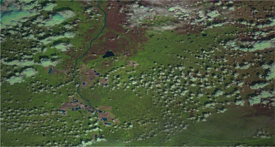
Figure 2. Raw color image. Images obtained from USGS/NASA Landsat Program.

FIGURE 3

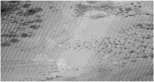
Figure 3. Thermal image. Images obtained from USGS/NASA Landsat Program.

The land-cover value is obtained by processing the satellite images in an open source geoprocessing software (Multispec). Temperature is obtained from processing thermal images from the same data source. Wind speed, rain, and wind direction are obtained from the historical datasets present in the Canada Information Portal² and World Clim datasets for the region of study. Relative humidity is obtained from processing satellite datasets from the USGS as explained in Peng et al. (2006).

The resolution for all the inputs was fixed to be 30 m in accordance with the spatial resolution of the satellite images. As all the other information came from data sources that have lesser resolution that 30 m all the inputs were comfortably generalized to 30 m. For example, the initial state of the Richardson fire contained the following values for a particular spatial location (fixed x, y) and calendar day. Date = May 8, 2011, geographic coordinates (x, y) = (57°24′11.2″ N, 111°13′20.8″ W), temperature (t) = 10.1 C, land cover (l) = vegetation (black spruce), wind speed (w) = 8.05 mph, wind direction (d) = NW, rainfall (r) = 35.1 mm, and relative humidity (rh) = 50%.

4. Definition of Algorithms

We compare five very different, widely used RL algorithms on this domain to see the range and application of the idea. We begin with three classic approaches for iteratively solving MDPs, value iteration, policy iteration, and Q-learning. We then consider the recent and very different approaches of Monte Carlo Tree Search and A3C, a recent policy gradient RL algorithm that utilizes deep Learning for value function representation. These algorithms will be reviewed briefly with modifications needed for our problem highlighted.

For all of the following methods each cell in the target area that is visited has the resulting value estimate stored in a hash data structure so it expands only as new states are encountered.

4.1. Asynchronous Value Iteration (VI)

The optimal value of the state V*(s) under the greedy fire spread policy is given by the following Bellman equation:

$V^{\ast }(s)=R(s)+{\text{max}}_a\gamma {\displaystyle \sum _{s^{\prime }}}P(s^{\prime }\mathrm{|}s,a)V^{\ast }(s^{\prime })$ (1)

where s′ is the successor state and γ denotes the discount factor which we set to 0.9. States are randomly sampled to update the value function according to equation (1) and updates are stopped when the change in value made by the successive iterations is less than 0.1. To provide a signal for training, a pixel in the center of the region of consideration that is currently burning in the next time step is given a high positive reward. This can be considered the goal state to reach for the burning cell as in a classic navigation problem using RL. This approach is utilized for training both value and policy iteration algorithms.

4.2. Policy Iteration (PI)

We begin with an initial random policy for acting in each state and iteratively improve it through alternating policy evaluation 2 and improvement 3 steps defined as follows:

$V_{\pi }(s)=R(s,{\pi }_{(s)})+\gamma {\displaystyle \sum _{s^{\prime }\in S}}T(s,\pi (s),s^{\prime })V_{\pi }(s^{\prime })$ (2)

${\pi }_{k+1}(s)={\text{argmax}}_a{\displaystyle \sum _{s^{\prime }}}T(s,a,s^{\prime })[R(s,a,s^{\prime })+\gamma V_i^{{\pi }_k}(s^{\prime })]$ (3)

The discount factor γ was fixed to be 0.9. For this algorithm, the value function V_π(s) is an array of Net Policy Worth values for all states, which is the highest cumulative reward that could be obtained for an optimal policy passing through that state. This is required to maintain single-step dynamics since each cell could take more than one action at a time as fire spreads in multiple directions.

4.3. Q-Learning (QL)

This algorithm (Watkins, 1989) performs off-policy exploration and uses temporal differences to estimate the optimal policy. In Q-learning, the agent maintains a state-action value function Q(S,A) instead of a state value function. This is updated as follows:

$\hat{Q}(s,a)=(r+\gamma (\text{max}Q(s^{\prime },a^{\prime })))$ (4)

and

$Q(s,a)=Q(s,a)+\alpha (\hat{Q}(s,a)-Q(s,a))$ (5)

where α denotes the learning rate and γ denotes the relative value of delayed vs immediate rewards. S′ is the new state after action a. a and a′ are actions taken in states s and s′, respectively. max_a Q(s′, a′) denotes the estimate of maximum discounted future reward expected.

The learning rate for Q-learning was chosen to be 0.9 as we need the most recent information to have a higher impact in a continuous spatial environment like that of forest fire. There is a high positive spatial auto-correlation in spatial datasets corresponding to fire as the similar pixels(on fire or not fire) tend to cluster together. The Q-learning is made to exploit this property using the appropriate learning rate. The discount factor is determined to be 0.9 as the long-term rewards are more important than the short-term rewards in our model and we want the model to converge. Using a lower discount rate decreases the level of exploration and the risk of falling into a local optimum becomes high. Each state-action pair is considered as a step taken in the real world. For every valid state, the highest Q value (utility value) for the state is recorded. The burned area is determined to be all the states having utility values over the threshold. Further, for each successive time step in the real world, a suitable number of steps taken by the fire are determined approximately using the difference between the total number of cells being burnt between successive time steps and is used to cap the total number of steps (state—action pairs analyzed) in the Q-learning implementation for the time step at which the learning is taking place. This is done to obtain a faster convergence.

4.4. Monte Carlo Tree Search (MCTS)

These are a class of algorithms that perform approximate, but confidence-bounded, RL by performing short roll-outs of the current policy to obtain enough statistical information about a state to keep it or discard it as belonging to the optimal path. A good survey is provided in Browne et al. (2012).

In our implementation of MCTS, each node in the search tree is a valid cell state in the fire model. From each state, any possible action could be taken, which is modeled as branches in the tree. The nodes in the tree are made to be selected by the Upper Confidence Bound for trees (UCT) (Kocsis and Szepesvári, 2006) method to minimize the cumulative regret. Each “step” in the MCTS tree is defined as a possible action taken from any valid state. A correlation between number of steps a fire can take in a 16-day period has been worked out empirically to be about 1,000. So, the MCTS roll-out policy is forced to stop after taking 1,000 steps. Note that there is a stay action defined for every fire location. Thus, in this implementation, it is possible to go a few levels down the tree without that corresponding to any real action in the world. Rewards are given based at each step of the roll-out and when complete the combined reward is used to update the value for the initial state at the root of the roll-out tree. For computational simplicity, during the roll-out a simpler state representation is used which focuses only on number of cells burning.

4.5. Deep RL

The final comparison is using the Asynchronous Advantage Actor-Critic (A3C) algorithm (Mnih et al., 2016), which represents the state-action value function using a Deep Q-Network (DQN) (Mnih et al., 2013). This algorithm defines a global network in addition to multiple worker agents with individual sets of parameters. The input to this global network was formalized as a grid of 100 × 100 cells with each cell having state values, which is an average of the state values of several pixels derived from satellite images. For our problem, A3C has the advantage of defining multiple worker agents. Each separate instance of a fire (unconnected to other fires) in a neighborhood is given its environment as an input, and the fire is defined as an individual worker. In our data, there are 96 instances of fire (thus, 96 worker agents) considered for training and testing. Each worker would then update the global environment, and we have plotted the result obtained. The deep network used is based on the DQN network given in Mnih et al. (2013), which uses an input layer of 100 × 100 pixel windows from the satellite image for the start date. Then there is a convolution layer of 16, 8 × 8 filters with a stride of 4 followed by a rectifier nonlinear unit (ReLU) layer. The second hidden layer involves 32 4 × 4 filters using a stride of 2 also followed by a ReLU layer. The final fully connected layer uses 256 ReLUs, which is output to a layer of threshold functions for the output of each of the five possible actions.

5. Supervised Classification—Gaussian Process

In this supervised classification method of performing the experiments, the Gaussian process algorithm (Rasmussen and Williams, 2006) is used to estimate if a particular cell is burning or not based on the burning conditions of other cells in the scene. For each particular cell, the attributes of temperature, rain, relative humidity, land-cover type, wind speed, and wind direction are considered to influence the decision.

A distribution over function f can be specified by the Gaussian process as given by:

$p(f)=GP(f|0,k(x,x^{\prime })),$

where the mean function is 0, and the covariance is defined by some kernel function. We use the RBF kernel in our experiments because we have an assumption of 2D proximity of features being relevant in any direction.

The GP prior is a multivariate normal given by:

$p(y)=Normal(y|0,K),$

where K is a covariance matrix given by evaluating k(x_n, x_m) for each pair of inputs. The mean of the GP prior is assumed to be 0 in accordance with the above equations.

To obtain a probability the output response is condensed into the range [0, 1], which is an appropriate choice for classification. The probability is given by the condensed value, and a Bernoulli distribution is used to determine the label.

The likelihood of an observation (x_n, y_n) is given by:

$p(y_n|z,x_n)=Bernoulli(y_n|logi{t}^{-1}(z_n)).$

Gaussian processes were chosen for this problem as they are known to work well for modeling non-linear relationships between variables especially in spatial domains. For the GP classifier, we use the logistic (sigmoid) function, whose integral is approximated for the binary case to map output to a probability. For the covariance function, we use an RBF kernel (stationary kernel) because we have an assumption of 2D proximity of features being relevant in any direction. The hyper-parameters of the kernel are optimized by maximizing the log-marginal-likelihood of the optimizer. A Cholesky decomposition was used to decompose the kernel matrix. The result is a binary output response, which can be used for classification.

6. Experimental Setup

To evaluate this idea of agent-based RL for SSP prediction, we performed a cross-comparison of five RL algorithms and a supervised spatial GP approach using a two-stage training process. In the first stage, we learn the cell-based fire spread policy directly using the satellite images from the start of the fire and the image at its next successive time step. This is the policy from the MDP, which describes spread of fire from one cell to another based on local conditions. The training data images are spaced 16 days apart, so many successive calls to this policy are required to reach the fire spread for 16 days. Thus, the second stage of training is to choose a cap C for the number of calls to this policy to obtain the correct spread area. We use another future satellite image to choose this cap based on maximum number of cells the policy got correct. The cap is used to set the upper limit of the total number of moves in any experiment.

In experiment (A), we test the ability of the algorithms to learn the spread of fire in an intermediate time step if the previous and next time step are known. Thus, we optimize C based on the ground truth data for time step 3. Now, the learned policy and the cap are used to determine the fire spread at the intermediate step 2 given that this is halfway between the state reached in step 3.

In experiment (B), we start with the initial state of the fire, we provide rewards based on the time step 2 of the fire, and we ask the algorithm to predict time step 3. This experiment is similar to asking the question: Where will the fire spread in the next 16 days, given its position currently? In this case, the cap value C is tuned for a 16-day duration.

In experiments (C)–(F), we apply the learned policy from the Richardson fire to the Fort McMurray fire over four 16-day time steps but tune the cap value C using the first transition in the Fort McMurray data. This was a fire that happened in Northern Alberta 5 years after the Richardson fire used for training. As the regions are similar and very near each other, the general properties that the model encapsulates should remain relevant. The initial state for the Fort McMurray fire is provided in a similar way to the Richardson fire.

After limiting the number of calls in any experiment based on the cap, we need a policy that determines if a fire should spread from one burning cell to a nearby non-burning cell. For the RL algorithms, this is done by applying a threshold to the value function to determine spread or non-spread. This threshold is determined for each algorithm to balance true positives and false positives based on the training data. For all the experiments, the result from the algorithms in the form of burned areas is compared against the actual scenario, using the satellite images corresponding to the predicted time step.

All experiments were run on an Intel core i7-6700 CPU with 32GB RAM.

7. Analysis of Results

The task in these experiments is essentially to classify each cell at each time step correctly in terms of burning or not burning. So we can use the true positive rate and false positive rate to compute a receiver operating curve (ROC) and a corresponding area under the curve (AUC) metric. The AUC for experiment (A) is shown in Table 1 for all algorithms and shows that the A3C algorithm provides an excellent threshold while classic value iteration is the least favorable. This seems to augur well with the overall accuracy for experiment (A) seen in Table 2.

TABLE 1

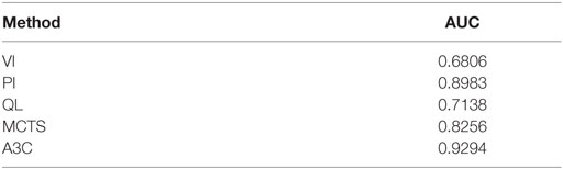
Table 1. AUC for all the methods.

TABLE 2

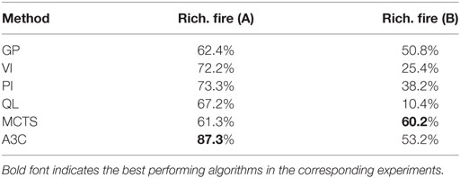
Table 2. Average accuracy for each algorithm on the different test scenarios.

Figures 4 and 5 show the visualization of some of the results for the different experiments. For all the images, the red pixels correspond where fire was classified correctly, blue pixels represent those which were classified as burning but were not yet at that point. White pixels represent false negatives where the policy predicted no fire but fire was indeed present. Black pixels represent true negatives, the pixels that were not on fire and correctly classified.

FIGURE 4

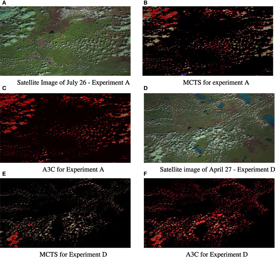
Figure 4. Results for experiments from the best two algorithms MCTS and A3C for filling in an (intermediary state) in the training region (A) and applying that policy in a different region (D). Red pixels were on fire and classified correctly (true positives), blue pixels were incorrectly classified as burning (FP), white pixels were incorrectly classified as not burning (FN), and black pixels were correctly classified as not burning (TN). (A) Satellite image of July 26—experiment (A). (B) MCTS for experiment (A). (C) A3C for experiment (A). (D) Satellite image of April 27—experiment (D). (E) MCTS for experiment (D). (F) A3C for experiment D. Images obtained from USGS/NASA Landsat Program.

FIGURE 5

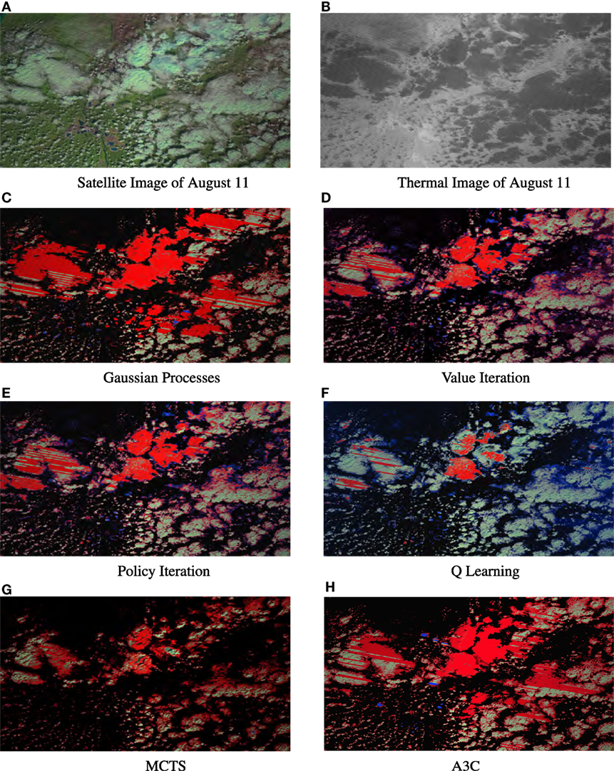
Figure 5. Results for experiment (B) from all algorithms showing performance on the prediction of the next state directly after the training data. (A) Satellite image of August 11. (B) Thermal image of August 11. (C) Gaussian processes. (D) Value iteration. (E) Policy iteration. (F) Q-learning. (G) MCTS. (H) A3C. Images obtained from USGS/NASA Landsat Program.

From all the algorithms considered, A3C seems to be the best overall, which is not surprising as it has the most flexible state-action value function representation. Policy Iteration in general comes second best in most tests. Q-learning a model free method of learning gives a lesser accuracy than model-based approaches like Value and Policy Iteration. In a spatial domain, the environment has a high influence on the spread of the agent. Thus, the strong consideration of the model of the spatial environment helps the model-based approaches.

The output images in Figures 5G,H show the two most successful algorithms MCTS and A3C on the region on which they were trained, filling in fire predictions between the start state and the reward target. Looking at the output images in Figures 4E,F, we see these two algorithms applied to the Fort McMurray fire (similar region, different year, and not part of the training data) at the same number of days forward after the start state. We can see that the model trained on one set images applies quite well to a different start state it has never seen, but A3C has much fewer false positives than MCTS. Figure 5 visualizes the results of all the RL algorithms on predicting the next time step after the training data on the Richardson fire, here A3C clearly produces the most accurate prediction.

Somewhat surprisingly, MCTS outperforms A3C in experiment (B) for forward prediction of the next 16-day period on the same location as the training data. It seems that the MCTS rollouts have fit a better model to the sense of real world “time” to predict the extent of a fire in the next time period. As can be seen for the results for (C) and (D) in Table 3, the A3C algorithm outperforms all others on prediction when the learned policy for one location is applied to another location in the same region. MCTS does significantly worse in this challenge, meaning its model is not as good at generalizing the essentials of the policy for transfer to a new location even though it seems to have a better model of dynamics.

TABLE 3

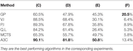
Table 3. Average accuracy of each algorithm trained on the Richardson fire but applied on the Fort McMurray fire for different time durations.

Note that the accuracy of all algorithms reduces with increasing time after the start of a fire as can be see by looking at experiments (C)–(F) in Table 3. This is unsurprising, as predicting multiple steps into the future is inherently harder. However, it is also partially due to the fact that later fires are larger, more intense, and spread faster, making learning more difficult. In the first time step, all algorithms do very well as it is easier to predict the first few moves of the fire. The accuracy goes down rapidly, and in the last time step it is only around 10%.

It is also interesting to note that even though MCTS starts of with a low accuracy compared with the other methods in the first time step, its cautious approach causes its accuracy to decrease much slower than other methods so that it seems tied with A3C when predicting three steps ahead. Similarly, the supervised GP method that loses out in most comparisons does far better for the hardest problem of predicting four time steps (about 2 months) ahead after all other methods have degraded. The GP approach is purely spatial pattern learning, with no element of dynamics. So one possible explanation is that, GP’s with only a spatial model and no notion of time loses out when changes over time are relevant, but once we are so far ahead after the start of the fire a notion of time actually proves to be detrimental as the behavior of a very intense fire is difficult to correlate with time and the GP’s more accurate spatial model wins out.

Turning our attention to the running times, we ran all experiments on similar scale problems running with the same system resources and training took between 5 and 7.5 h for all algorithms. Q-learning was the fastest to finish execution and obtained reasonably results even when even training time was subjected to a threshold cutoff. So Q-learning is a good candidate algorithm for fast approximations for testing purposes. One unique aspect of A3C is that it can exploit multithreading of CPU cores rather than GPU acceleration. Each fire in our dataset could be run as its own thread allowing A3C use similar training time to obtain superior results. MCTS was the slowest algorithm we tried since it is not multithreaded and requires extra roll-out simulations and back propagation at every iteration.

There are several reasons why the best RL algorithms are more suited to such domains than supervised learning algorithms. The first reason is that, RL can model the spatial dynamics along with time in such domains. This enables RL to predict action choices using a policy tuned to a particular time of fire spread test as compared with supervised learning which estimates a model based on inputs and outputs only. The second reason being RL prepares a policy for the agent that takes actions which model the underlying causal fire behavior. The supervised learning algorithms do not have such a state-action mapping. Thus this RL approach should be able to learn a reasonable policy in data-scarce scenarios by focusing on the reachable state-action space only.

8. Challenges and Future Work

As expounded in Malarz et al. (2002), forest fire prediction requires additional information consisting of firefighting intervention (such as fire fighting strategy and time elapsed), which are not taken into consideration in this study, as we chose a study region having very minimal fire fighting. In future work, we aim to incorporate this kind of information as well as enriching the model by including more land characteristics such as moisture, slope, and directional aspect as state variables in individual cells. We will also perform a wider comparison against different existing wildfire models algorithms such as those in Castelli et al. (2015).

We also plan to investigate improvements to the structure of the Deep Neural Network policy representation to tailor it more closely to this kind of spatially spreading problem. For example, the relatively better behavior of the supervised GP approach on distance predictions where the dynamics approximation may be hindrance, suggest trying a hybrid approaches, learning a pair of models, one temporal and atemporal to achieve the best of both.

A severe challenge in the wildfire domain is the relative paucity of data compared with some other image analysis problems. While there are vast databases of satellite imagery, they are not all readily available and find the very small proportion which contains forest wildfires is not straightforward. This study has looked at a pair of fires in a well known region but future work will use data from more locales and automate the process of data collection. We will also look at flooding as a similar but more data-rich domains. This limited amount of image data is one reason, we chose to use a state feature extraction approach rather than learning on the entire image directly. There simply may not be enough images to learn effectively. However, a filter-based approach such as Convolutional Neural Networks (CNNs) applied directly to the images would be possible if we use small filters on the same scale as the local neighborhood we used in this study. We are currently trying this approach using a combination of CNNs and Recurrent Neural Networks to better encapsulate the effect of time on the fire.

9. Conclusion

In this work, we presented a novel approach for utilizing RL for learning forest wildfire spread dynamics directly from readily available satellite images. Our approach inverts the usual RL setup so that the dynamics of the MDP is a simple function of the fire spread actions being explored while the agent policy is a learned model of the dynamics of a complex spatially spreading process. Our results indicate that A3C is better at predicting spread dynamics at intermediate time steps and MCTS performs better while predicting the future spread. As the test data diverge from the training data and temporal changes become less relevant, such as when the intensity of fire increases, the fully supervised Gaussian process approach performs better than the RL algorithms.

The intersection between the decision-making tools of Artificial Intelligence, the pattern recognition tools of machine learning, and the challenging datasets of sustainability domains offers a rich area for research. For the machine learning community, our approach opens up new set of challenging and plentiful datasets for learning patterns of spatial change over time in the form of spatially spreading wildfires and a platform for experimenting with new Deep RL approaches on a challenging problem with high social impact.

We hope this can lead to development of a comprehensive way of integrating deep learning and RL approaches to support the tasks of prediction, dynamics model learning, and decision making in problems with SSP structure. This would also involve new representations for spatial data and policies, which can benefit theoretical as well as applied practitioners. Finally, the algorithmic approach demonstrated here could lead to more effective modeling and decision-making tools for domain practitioners in forest wildfire management which we are exploring with collaborators.

Author Contributions

SS was responsible for primary design of experiments, collection of data and results, implementation of the reinforcement learning algorithms, and writing. MC carried out high level design of the algorithms, experimental design, and writing.

Conflict of Interest Statement

The authors declare that the research was conducted in the absence of any commercial or financial relationships that could be construed as a potential conflict of interest.

Funding

This project has been funded by internal funds provided for research by the Electrical and Computer Engineering Department at the University of Waterloo. No external granting agency funding was used for this project. This project was also partially funded by a Mitacs Globalink Graduate Fellowship Award.

Footnotes

1. ^https://earthexplorer.usgs.gov/ (Accessed: December 5, 2016).
2. ^https://www.canada.ca/en/services/environment/weather.html (Accessed: December 5, 2016).

References

Alkhatib, A. A. (2014). A review on forest fire detection techniques. Int. J. Distrib. Sens. Netw. 10, 597368–597380. doi: 10.1155/2014/597368

CrossRef Full Text | Google Scholar

Angayarkkani, K., and Radhakrishnan, N. (2009). Efficient forest fire detection system: a spatial data mining and image processing based approach. Int. J. Comput. Sci. Netw. Secur. 9, 100–107.

Google Scholar

Browne, C. B., Powley, E., Whitehouse, D., Lucas, S. M., Cowling, P. I., Rohlfshagen, P., et al. (2012). A survey of Monte Carlo tree search methods. IEEE Trans. Comput. Intell. AI Games 4, 1–43. doi:10.1109/TCIAIG.2012.2186810

CrossRef Full Text | Google Scholar

Castelli, M., Vanneschi, L., and Popovič, A. (2015). Predicting burned areas of forest fires: an artificial intelligence approach. Fire Ecol. 11, 106–118. doi:10.4996/fireecology.1101106

CrossRef Full Text | Google Scholar

Cortez, P., and Morais, A. (2007). “A data mining approach to predict forest fires using meteorological data,” in Volume Proceedings of the 13th Portuguese Conference on Artificial Intelligence, Guimarães, Portugal.

Google Scholar

Cracknell, M. J., and Reading, A. M. (2014). Geological mapping using remote sensing data: a comparison of five machine learning algorithms, their response to variations in the spatial distribution of training data and the use of explicit spatial information. Comput. Geosci. 63, 22–33. doi:10.1016/j.cageo.2013.10.008

CrossRef Full Text | Google Scholar

Finney, M. A. (1998). Farsite: Fire Area Simulator-Model Development and Evaluation. Technical Report RMRS-4. Missoula, MT: USDA Forest Service, Rocky Mountain Research Station.

Google Scholar

Finney, M. A., Cohen, J. D., McAllister, S. S., and Jolly, W. M. (2013). On the need for a theory of wildland fire spread. Int. J. Wildland Fire 22, 25–36. doi:10.1071/WF11117

CrossRef Full Text | Google Scholar

Forsell, N., Garcia, F., and Sabbadin, R. (2009). “Reinforcement learning for spatial processes,” in 18th World IMACS/MODSIM Congress, Cairns, Australia, 755–761.

Google Scholar

Garzón, M. B., Blazek, R., Neteler, M., De Dios, R. S., Ollero, H. S., and Furlanello, C. (2006). Predicting habitat suitability with machine learning models: the potential area of Pinus sylvestris l. In the Iberian Peninsula. Ecol. Model. 197, 383–393. doi:10.1016/j.ecolmodel.2006.03.015

CrossRef Full Text | Google Scholar

Houtman, R. M., Montgomery, C. A., Gagnon, A. R., Calkin, D. E., Dietterich, T. G., McGregor, S., et al. (2013). Allowing a wildfire to burn: estimating the effect on future fire suppression costs. Int. J. Wildland Fire 22, 871–882. doi:10.1071/WF12157

CrossRef Full Text | Google Scholar

Jean, N., Burke, M., Xie, M., Davis, W. M., Lobell, D. B., and Ermon, S. (2016). Combining satellite imagery and machine learning to predict poverty. Science 353, 790–794. doi:10.1126/science.aaf7894

PubMed Abstract | CrossRef Full Text | Google Scholar

Kanevski, M., Pozdnukhov, A., and Timonin, V. (2008). “Machine learning algorithms for geospatial data applications and software tools,” in 4th International Congress on Environmental Modelling and Software, Barcelona, Spain.

Google Scholar

Knudby, A., LeDrew, E., and Brenning, A. (2010). Predictive mapping of reef fish species richness, diversity and biomass in Zanzibar using Ikonos imagery and machine-learning techniques. Remote Sens. Environ. 114, 1230–1241. doi:10.1016/j.rse.2010.01.007

CrossRef Full Text | Google Scholar

Kocsis, L., and Szepesvári, C. (2006). “Bandit based Monte-Carlo planning,” in European Conference on Machine Learning (Berlin, Heidelberg: Springer), 282–293.

Google Scholar

Kubat, M., Holte, R. C., and Matwin, S. (1998). Machine learning for the detection of oil spills in satellite radar images. Mach. Learn. 30, 195–215. doi:10.1023/A:1007452223027

CrossRef Full Text | Google Scholar

Li, J., Heap, A. D., Potter, A., and Daniell, J. J. (2011). Application of machine learning methods to spatial interpolation of environmental variables. Environ. Model. Software 26, 1647–1659. doi:10.1016/j.envsoft.2011.07.004

CrossRef Full Text | Google Scholar

Malarz, K., Kaczanowska, S., and Kuakowski, K. (2002). Are forest fires predictable? Int. J. Mod. Phys. C 13, 1017–1031. doi:10.1142/S0129183102003760

CrossRef Full Text | Google Scholar

Martell, D. L. (2015). A review of recent forest and wildland fire management decision support systems research. Curr. For. Rep. 1, 128–137. doi:10.1007/s40725-015-0011-y

CrossRef Full Text | Google Scholar

Mcgregor, S., Houtman, R., Buckingham, H., Montgomery, C., Metoyer, R., and Dietterich, T. G. (2016). “Fast simulation for computational sustainability sequential decision making problems,” in Proceedings of the 4th International Conference on Computational Sustainability, New York, 5–7.

Google Scholar

Mnih, V., Badia, A. P., Mirza, M., Graves, A., Lillicrap, T., Harley, T., et al. (2016). “Asynchronous methods for deep reinforcement learning,” in International Conference on Machine Learning, New York, 1928–1937.

Google Scholar

Mnih, V., Kavukcuoglu, K., Silver, D., Graves, A., Antonoglou, I., Wierstra, D., et al. (2013). Playing Atari with Deep Reinforcement Learning. CoRR, abs/1312.5602.

Google Scholar

Montgomery, C. (2014). “Chapter 13: fire: an agent and a consequence of land use change,” in The Oxford Handbook of Land Economics, eds J. M. Duke and J. Wu (Oxford University Press), 281–301.

Google Scholar

Peng, G., Li, J., Chen, Y., Norizan, A. P., and Tay, L. (2006). High-resolution surface relative humidity computation using Modis image in peninsular Malaysia. Chin. Geogr. Sci. 16, 260–264. doi:10.1007/s11769-006-0260-6

CrossRef Full Text | Google Scholar

Rasmussen, C. E., and Williams, C. K. (2006). Gaussian Processes for Machine Learning, Vol. 1. Cambridge: MIT Press.

Google Scholar

Recknagel, F. (2001). Applications of machine learning to ecological modelling. Ecol. Model. 146, 303–310. doi:10.1016/S0304-3800(01)00316-7

CrossRef Full Text | Google Scholar

Saranya, N. N., and Hemalatha, M. (2012). “Integration of machine learning algorithm using spatial semi supervised classification in FWI data,” in 2012 International Conference on Advances in Engineering, Science and Management (ICAESM) (Nagapattinam: IEEE), 699–702.

Google Scholar

Sehgal, V., Getoor, L., and Viechnicki, P. D. (2006). “Entity resolution in geospatial data integration,” in Proceedings of the 14th Annual ACM International Symposium on Advances in Geographic Information Systems (Arlington, Virginia: ACM), 83–90.

Google Scholar

Sitanggang, I. S., and Ismail, M. H. (2011). Classification model for hotspot occurrences using a decision tree method. Geomatics Nat. Hazards Risk 2, 111–121. doi:10.1080/19475705.2011.565807

CrossRef Full Text | Google Scholar

Stocks, B. J., Lynham, T., Lawson, B., Alexander, M., Wagner, C. V., McAlpine, R., et al. (1989). Canadian forest fire danger rating system: an overview. For. Chron. 65, 258–265. doi:10.5558/tfc65258-4

CrossRef Full Text | Google Scholar

Subramanian, S. G., and Crowley, M. (2017). “Learning forest wildfire dynamics from satellite images using reinforcement learning,” in Conference on Reinforcement Learning and Decision Making (Ann Arbor, MI).

Google Scholar

Sutton, R. S., and Barto, A. G. (1998). Reinforcement Learning: An Introduction. Cambridge, MA: MIT Press.

Google Scholar

Watkins, C. (1989). Learning from Delayed Rewards. PhD thesis, King’s College, Cambridge, UK.

Google Scholar

Woo, A., and Tait, C. (2016). Up to 90,000 Evacuated from Fort McMurray. The Globe and Mail.

Google Scholar

Yongzhong, Z., Feng, Z.-D., Tao, H., Liyu, W., Kegong, L., and Xin, D. (2004). “Simulating wildfire spreading processes in a spatially heterogeneous landscapes using an improved cellular automaton model,” in Geoscience and Remote Sensing Symposium, 2004. IGARSS’04. Proceedings. 2004 IEEE International, Vol. 5 (Anchorage, AK: IEEE), 3371–3374.

Google Scholar

Zhang, J.-H., Yao, F.-M., Liu, C., Yang, L.-M., and Boken, V. K. (2011). Detection, emission estimation and risk prediction of forest fires in china using satellite sensors and simulation models in the past three decades – an overview. Int. J. Environ. Res. Public Health 8, 3156–3178. doi:10.3390/ijerph8083156

CrossRef Full Text | Google Scholar