Chlorophyll variability in the oligotrophic gyres: mechanisms, seasonality and trends

Introduction

Subtropical gyre variability as seen from ocean color satellites has been analyzed in previous studies. McClain et al. (2004) showed that the oligotrophic waters of the North Pacific and North Atlantic gyres were observed to be expanding, while those of the South Pacific, South Atlantic and South Indian Ocean gyres show much weaker and less consistent tendencies. Their results were based on 8 months (November 1996–June 1997) of Ocean Color and Temperature Sensor (OCTS) and 6 years (September 1997–October 2003) of Sea-viewing Wide Field-of-view Sensor (SeaWiFS) ocean color data. Polovina et al. (2008) used a 9-year (1998–2006) time series of SeaWiFS to examine temporal trends in the oligotrophic areas of the subtropical gyres. They concluded that in the 9-year period, in the North and South Pacific, North and South Atlantic, outside the equatorial zone, the areas of low-surface chlorophyll waters had expanded at average annual rates from 0.8% to 4.3%. In addition, mean SST in each of these 4 subtropical gyres increased over the 9-year period, with the expansion of the low-chlorophyll waters being consistent with global warming scenarios based on increased vertical stratification in the mid-latitudes.

An important biological characteristic of the subtropical gyres is the large variability in phytoplankton growth rates with minimal changes in biomass (Laws et al., 1987; Marra and Heinemann, 1987; Marañón et al., 2000, 2003). Therefore, understanding the interactions between physical and biological processes within the subtropical gyres is central for determining the magnitude and variability of the carbon exported from the surface to the deep ocean.

We used a satellite multi-sensor approach to analyze the biological response of all 5 subtropical gyres to changes in physical forcing. A major data source for our analysis was the chlorophyll-a (Chl-a) combined data from SeaWiFS and the Moderate-resolution Imaging Spectroradiometer (MODIS) on Aqua, which together provided 16 years of continuous high-quality global data. Satellite-based SST data were obtained from optimally interpolated (OI) Advanced Very High Resolution Radiometer (AVHRR) data (Reynolds et al., 2007) and dynamic height (h) from altimetry data. The results reported in this article are based on data records that are longer than the ones used in similar previous efforts (McClain et al., 2004; Polovina et al., 2008; Signorini and McClain, 2012). These previous studies reported significant changes in the sizes of most gyres. The seasonal cycle and long-term trends of the physical forcing and biological response are analyzed within the geographical domain of the subtropical gyres, based on the most recent reprocessing of the entire SeaWiFS data record (1998–2010) combined with MODIS data for the period of 2011–2013, the longest (16 years) ocean color record of adequate data quality for this analysis.

Methodology

The study domains for all 5 gyres, the North and South Pacific (NPAC and SPAC), the North and South Atlantic (NATL and SATL) and the South Indian Ocean (IOCE) gyres, are shown in Figures 1–3 as polygons bounded by white lines. The choice for the gyre domain polygons follows the methodology of Signorini and McClain (2012). The oligotrophic regions (purple areas in Figure 1A) expand during summer and contract during winter following the seasonal strength of the winds and convective upper-ocean mixing. The rationale for choosing the size and shape of the study polygons is twofold: (1) they should contain the entire oligotrophic regions of the gyres during the maximum expansion in summer and (2) they should avoid peripheral regions where other dynamic processes prevail, such as coastal and equatorial upwelling, river discharge and western and eastern boundary current systems.

FIGURE 1

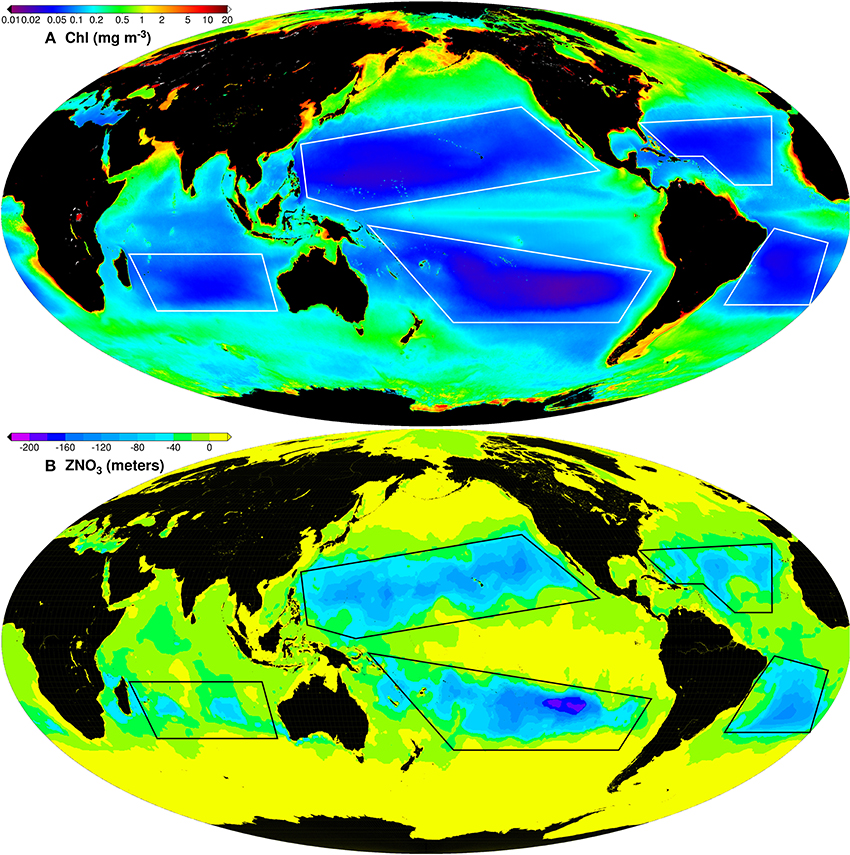
Figure 1. Global maps of 9 km MODISA OCI Chl-a mission composite (A) and the depth of the 0.2 μM (ZNO₃) nitrate concentration (B) derived from the World Ocean Atlas monthly climatology. The transition to the yellow color in (B) indicates that the 0.2 μM nitrate horizon has reached the surface. The polygons represent the study areas of the 5 gyres.

Data Sources and Processing

Our analysis is based on five satellite data sources spanning the common period of 1998–2013. These include the combined time series of 9 km monthly Chl-a from the latest SeaWiFS and MODIS reprocessing (http://oceancolor.gsfc.nasa.gov/), 0.25° daily NOAA optimally interpolated (OI) SST, and Aviso 0.25° daily h from multi-sensor altimetry. Finally, we used global monthly net primary production from the updated Carbon-based Production Model-2 (CbPM2) to derive the combined SeaWiFS-MODIS (1998–2013) net primary production (NPP) time series for all gyres. The resolution of the NPP monthly grids is ~18 km and a detailed description of the CbPM2, with vertically resolved photoacclimation, is given in Westberry et al. (2008). The SST and h products were averaged to monthly values after the daily SST and h time series of gyre domain averages were computed. Seasonal climatology and time series of averaged Chl-a, SST and h were produced within the limit domains of all 5 gyres. The anomalies of each parameter were then calculated by removing the seasonal climatology from the time series and long-term trends were derived for each parameter and gyre domain. The statistical analysis for the trends was done with MatLab using the regression diagnostics function “regstats” using a linear regression model.

In addition, mixed-layer time series data were derived from gridded temperature and salinity profiles (1998–2010) available from the Simple Ocean Data Assimilation (SODA) model (Carton et al., 2000) on a global 0.5 degree grid. The water density was calculated from the SODA temperature and salinity profiles and the monthly MLD were calculated using a critical density threshold of 0.03 kg m⁻³.

MODIS and SeaWiFS chlorophyll and NPP

The global monthly Chl-a and NPP products used in this study were derived from NASA standard products of spectral water-leaving “remote sensing” reflectance over the visible spectral regime, Rrs(λ), associated with MODIS-Aqua version 2013.1 and SeaWiFS version 2010.0. The Rrs(λ) were produced by NASA using common algorithms and methods to maximize consistency across the two missions (Franz et al., 2012), with MODIS updated more recently to incorporate improved instrument temporal calibration knowledge (Meister and Franz, 2014).

For both SeaWiFS and MODIS, the STD Chl-a product uses a blue to green band ratio algorithm to relate Rrs (λ) to Chl-a that has been shown to perform well over a wide dynamic range of Chl-a (O'Reilly et al., 1998, with empirical coefficients updated via Werdell and Bailey, 2005). The recently developed OCI algorithm (Hu et al., 2012) is an alternative approach specifically developed to improve retrievals in low Chl-a waters. OCI uses a line-height approach wherein the Chl-a is related to the difference between Rrs (green) and a linear baseline from Rrs (blue) to Rrs (red). The advantage of this line-height approach is that it is robust to spectrally correlated biases, such as those associated with atmospheric correction error or residual sun glint contamination that can dominate the very low green reflectance in clear waters and thus drive-up uncertainty in the STD blue to green band ratio. OCI is therefore a logical choice for this study of ocean gyres, but the STD Chl-a time-series is also assessed, as that algorithm was used in all previous studies (McClain et al., 2004; Polovina et al., 2008; Signorini and McClain, 2012).

The SeaWiFS mission operated from late 1997 to late 2010, with some periods of sporadic operations in the latter 3 years, while MODIS-Aqua began operations in 2002 and continues to this day. This study thus makes use of a merged SeaWiFS-MODIS Chl-a and NPP time-series to span the period from 1998 to 2013, as derived from the consistently-processed monthly Rrs (λ). Specifically, the SeaWiFS monthly products were used exclusively from 1998 through 2007, MODIS was used exclusively from 2011–2013, and MODIS was used in the 2008–2010 period for those months where SeaWiFS data was incomplete or unavailable. Previous studies have demonstrated a high level of consistency between the STD Chl-a products of SeaWiFS and MODIS for global ocean regions (Franz et al., 2012, 2014), thus providing some confidence in the use of a merged time-series for trend analysis, but additional analyses were performed here to specifically assess the mission to mission consistency within the study domain.

Dynamics and Biogeochemical Characteristics of the Subtropical Gyres

Although the subtropical gyres are characterized by oligotrophic waters (low biomass and production), and are quite often referred to as the ocean deserts, their immense size (they occupy ~ 40% of the surface of the earth) makes their contribution to the global carbon cycle very important. The upper kilometer of the subtropical gyres circulation is primarily wind driven (Huang and Russell, 1994). The horizontal and vertical motion in this layer plays a significant role in controlling the interaction between the atmosphere and ocean, which is of vital importance to our understanding of the oceanic general circulation and climate (Huang and Qiu, 1994). The gyres are characterized by a deep pycnocline at their centers and strong horizontal gradients of temperature and salinity at the fringes due to pycnocline outcropping. The flow in the western limbs (western boundary currents) is intensified by the latitudinal changes of the Coriolis acceleration (βeffect), whereas the flow is relatively weak in the gyres' eastern parts. The broad region of relatively weak flow occupies most of the gyre and is called the Sverdrup regime (Pedlosky, 1990). The dynamic center of the gyres can be identified by a maximum sea-surface height (SSH). The pycnocline shoals in the mid-latitudes, where isopycnals outcrop at the subtropical front, and at the equator, where Ekman flow divergence promotes upwelling. The interior of the gyres are also characterized by Ekman downwelling. McClain and Firestone (1993) provide evidence of gyre downwelling in the North Atlantic.

The availability of light and nutrients is the driver for phytoplankton photosynthetic carbon production. In the interior of the gyres the depth of the nutricline is much deeper than in its fringes as a result of gyre dynamics. This limits the availability of nutrient renewal within the euphotic zone as the vertical mixing needs to penetrate much deeper to reach depths were nutrients are more concentrated, thus limiting phytoplankton growth. This is clearly illustrated in Figure 1 which shows the MODIS mission composite global Chl-a map and the global nutricline horizon defined by the level at which the nitrate (NO3) concentration reaches 0.2 μM (ZNO₃). Areas inside the gyres have the clearest waters (low biomass) which are well correlated with the areas of deepest ZNO₃. The most distinctive feature of the phytoplankton size structure in these oligotrophic domains is the marked dominance of picoplankton (Marañón et al., 2001).

Previous studies indicate that the subtropical gyres undergo seasonal changes in the physical forcing and ecosystem response that alter the ratio of new vs. regenerated production. Brix et al. (2006) discussed the relationships between primary, net community, and export production in the subtropical gyres. They analyzed more than 10 years of data from two subtropical time-series stations (Hawaii Ocean Times-series (HOT) in the North Pacific, and Bermuda Atlantic Time-Series (BATS) in the North Atlantic) to investigate the regeneration loop vs. export pathway hypothesis, and in particular to test the idea that the switch between the two is controlled by enhanced input of nutrients. In the decadal long-term mean, their study revealed export pathway characteristics at BATS, while at HOT production is dominated by the regeneration loop. This difference is consistent with stronger seasonal forcing at BATS leading to enhanced nutrient input. However, these characteristics are only valid for parts of the year. Especially at BATS, the export pathway exists only in spring and the system reverts to a regeneration loop in summer and fall. This is a consistent result given the strong summer-time stratification and the resulting low levels of nutrient input.

Heat and freshwater (precipitation-evaporation) fluxes, combined with the gyre circulation, are the dynamic drivers for SST and sea surface salinity (SSS) spatial and temporal variability that highly influence vertical mixing and thus the depth of the mixed layer. Figure 2 shows global maps of MODIS SST and Aquarius SSS mission composites. There is large SST variability in the NPAC and SPAC gyres with warmest SSTs in the western equatorial region (Warm Pool) and significant decrease in SST toward the subtropical frontal regions. The Aquarius SSS global map shows that the surface salinity within the Atlantic gyres is greater than the salinity in the Pacific gyres. The mean Aquarius SSS for the NPAC, SPAC, IOCE, NATL and SATL are 34.620, 35.364, 35.125, 36.753, and 36.571, respectively. The mean SSS in the NATL gyre is about 2 psu higher than the mean SSS in the NPAC gyre. The mean SSS seasonal cycle of the NATL gyre has a range of ~0.3 psu, while the SATL and NPAC ranges are ~0.2 psu and the SPAC and IOCE have still smaller ranges (~0.1 psu or less). The minimum SSS occurs in summer-fall and the maximum in winter-spring for all gyres, except for the SATL gyre where the SSS seasonal cycle is in phase opposition with the other 4 gyres. This may be due to a different seasonality pattern of precipitation-evaporation in the sub-tropical SATL. The variability in surface water density due to changes in SST and SSS, combined with wind stirring, are effective drivers of vertical mixing, which in turn control the renewal of nutrients within the euphotic zone.

FIGURE 2

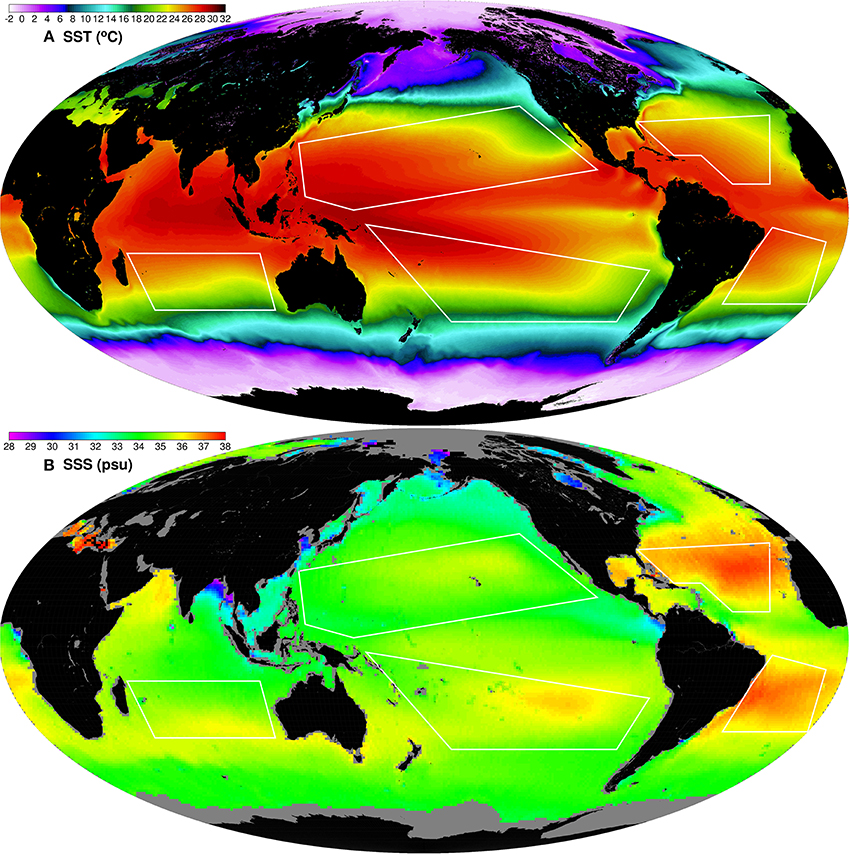
Figure 2. Global maps of 9 km MODISA SST mission composite (A) and Aquarius 1-degree SSS based on the August 2011–July 2013 composite (B).

A climatological global map of mixed layer depth (MLD) is shown in Figure 3A. There is a large spatial variability of MLD globally and within the gyres, a result of the interplay of the driving factors described above. The anti-cyclonic circulation patterns within the gyres are clearly shown in the climatological global map of Aviso dynamic height (Figure 3B), with the strongest western boundary currents being the Gulf Stream in the North Atlantic and the Kuroshio Current in the North Pacific, both originating from the western limbs of the gyres.

FIGURE 3

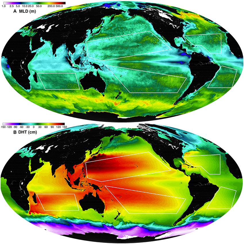
Figure 3. Global maps of climatologic (1998–2010) SODA MLD (A) and Aviso dynamic height climatology (1998–2013) based on the sum of SLA and mean dynamic topography (B).

Gyre-averaged seasonal plots of MODIS Chl-a, MLD, and ZNO₃ (Figure 4) provide evidence of the biogeochemical forcing vs. response behavior within the gyres. Note that the time axes have been adjusted to provide synchronization of seasons between the northern and southern hemispheres, so winter, summer, spring and autumn appear in phase in all gyres. Summer and autumn, a period of relatively shallower MLDs, are the seasons with lowest biomass (Chl-a), while in the peak of winter strong vertical mixing drives the elevated biomass shown by the higher values of Chl-a. Also note that Chl-a increases as the MLD gets deeper than ZNO₃.

FIGURE 4

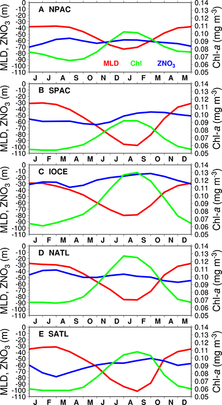
Figure 4. Seasonal variability of MODISA OCI Chl-a (green), mixed layer depth (MLD, red), and depth of the 0.2 μM nitrate concentration (ZNO₃, blue) for the 5 gyres (A through E for the NPAC, SPAC, IOCE, NATL, and SATL, respectively). Values were averaged within the polygons shown in Figure 1.

Results

MODIS vs. SeaWiFS Chl Trends

Individual mission-long MODIS (July 2002—May 2014) and SeaWiFS (1998–2010) monthly time-series Chl-a anomaly trend analyses, as well as trend analyses for the combined MODIS and SeaWiFS (1998–2013) monthly time series record, were performed using both STD and OCI algorithms. The trends and corresponding statistical results are summarized in Table 1.

TABLE 1

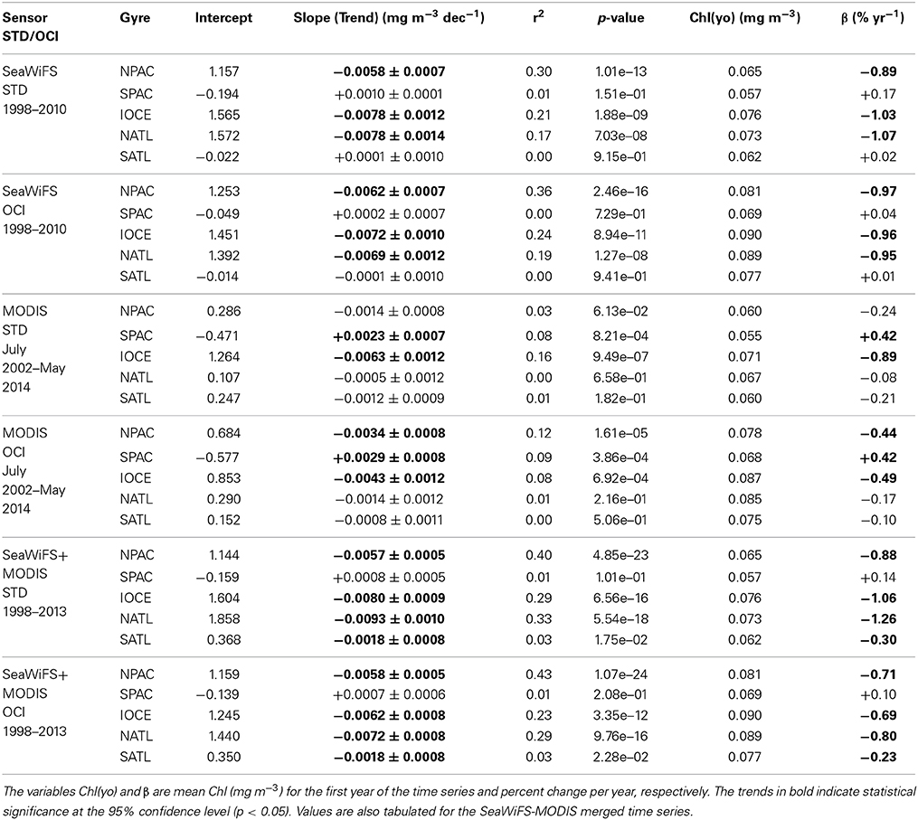
Table 1. Mission-long trends (mg m⁻³ decade⁻¹) for SeaWiFS and MODIS using STD and OCI Chl-a.

There is a general agreement of magnitude and sign of trends among the different sensors and algorithms, with some exceptions. The SPAC and SATL gyres are the only ones with positive trends, albeit with low statistical significance (p > 0.05). These 2 gyres show positive trends for the 13-year SeaWiFS record using both STD and OCI algorithms, while only the SPAC gyre shows consistent positive (weaker) trends for all other combinations of sensors and algorithms. The statistical significance for the trends is improved for some gyres when the longer MODIS-SeaWiFS 16-year combined record is used, except for the SPAC gyre which still shows a weaker positive trend with low statistical significance.

The trends for the 16-year record using the STD algorithm are −0.0057, +0.0008, −0.0080, −0.0093, and −0.0018 mg m⁻³ decade⁻¹ for the NPAC, SPAC, IOCE, NATL, and SATL gyres, respectively. The equivalent trends using the OCI algorithm are −0.0058, +0.0007, −0.0062, −0.0072, and −0.0018 mg m⁻³ decade⁻¹. The percent differences between the trends using the STD and OCI algorithms (based on 5 decimal places on the trends) are −1.2%, −12.7%, +28.8%, +29.0%, and +5.1% for the NPAC, SPAC, IOCE, NATL, and SATL gyres. The largest differences in trends between the IOCE and NATL gyres using the two different algorithms may be a result of stronger variability in the Chl-a anomalies in these 2 gyres (see Figure 5). There are several factors that contribute to the uncertainty associated with the estimation of the trends in the subtropical gyres, including sensor and algorithm accuracies and the length of available ocean color records.

FIGURE 5

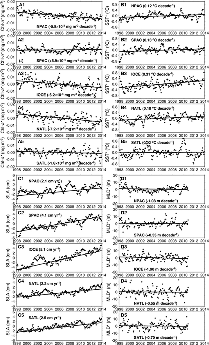
Figure 5. Trends of gyre anomalies for chlorophyll (Chl*, A1–A5), sea-surface temperature (SST*, B1–B5), sea-level anomaly (SLA, C1–C5), and mixed layer depth (MLD*, D1–D5) for all 5 gyres.

Gregg and Rousseaux (2014) analyzed decadal trends in global pelagic chlorophyll by integrating multiple satellites, in situ data, and models. Although they did not present averaged trends for the subtropical gyres in their trend analysis, their North Central Pacific (NCP) and North Central Atlantic (NCA) regional domains contain the NPAC and NATL oligotrophic regions analyzed in this study. Their NCP and NCA regions showed Chl downward trends of −1.1 and −1.4% yr⁻¹ for 1998–2012, respectively. As shown in Table 1, the Chl trends derived in this study are very close to those reported by Gregg and Rousseaux (2014). The Chl downward trends from SeaWiFS for the 1998–2010 period are −0.9 (STD Chl) to −1.0% yr⁻¹ (OCI Chl) for the NPAC, and −1.0 (OCI Chl) to −1.1% yr⁻¹ (STD Chl) for the NATL. The trends for 1998–2013 derived from the merged SeaWiFS-MODIS data are −0.7 (OCI Chl) to −0.9% yr⁻¹ (STD Chl) for the NPAC, and −0.8 (OCI Chl) to −1.3% yr⁻¹ (STD Chl) for the NATL.

Trend Analysis of Chl, NPP, SST, SLA, and MLD

The trends in Chl*, NPP*, SST*, SLA, and MLD* for all gyres, where the asterisk denotes anomalies, are presented in Table 2. The Chl* trends are tabulated for both the STD and OCI algorithms. The analysis was done using monthly data for the period of 1998–2013, except for the MLD which was limited by data availability (1998–2010). The units for the trends are chosen to enable uniform magnitude range and number of decimal places for all variables. The time series of monthly anomalies with superposed linear trends are shown in Figure 5 for all variables analyzed.

TABLE 2

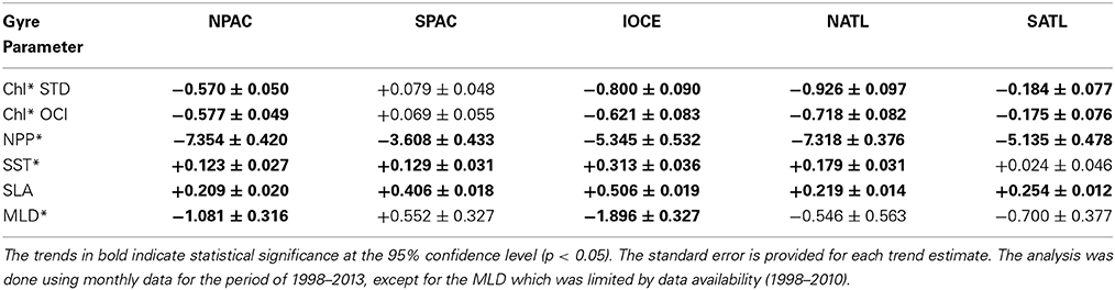
Table 2. Trends and statistics for Chl-a anomaly (Chl* in μg m⁻³ yr⁻¹) from SeaWiFS-MODIS combined data record using STD and OCI algorithms, CbPM net primary production anomaly (NPP* in mg C m⁻² d⁻¹ yr⁻¹), AVHRR optimally interpolated (OI) SST anomaly (SST* in °C decade⁻¹), Aviso sea level anomaly SLA (cm yr⁻¹), and mixed layer depth anomaly (MLD* in m decade⁻¹) derived from SODA temperature and salinity profiles.

As previously mentioned, the SPAC is the only gyre with a positive trend. It ranges from +0.069 to +0.079 μg m⁻³ yr⁻¹. All the other gyres have negative trends indicating an expansion of the oligotrophic areas. The SATL gyre has the weakest trend ranging from −0.175 to −0.184 μg m⁻³ yr⁻¹, while the NATL gyre has the strongest trend with values ranging from −0.718 to −0.926 μg m⁻³ yr⁻¹. The IOCE gyre has the second strongest negative trend ranging from −0.621 to −0.800 μg m⁻³ yr⁻¹. The warming trends in the gyres range from +0.123°C decade⁻¹ in the NPAC gyre to +0.313°C decade⁻¹ in the IOCE gyre, while the positive trend in the SATL gyre is relatively small and statistically insignificant. The SLA trends are also positive for all gyres, ranging from +0.209 cm yr⁻¹ in the NPAC gyre to +0.506 cm yr⁻¹ in the IOCE gyre. NPP trends are negative for all the gyres, −7.35, −3.61, −5.35, −7.32, and −5.14 mg C m⁻² d⁻¹ yr⁻¹ for the NPAC, SPAC, IOCE, NATL and SPAC, respectively.

The MLD* gyre trends, which were derived from the SODA model density profiles, have signs that agree with the signs of the Chl* trends. A positive MLD* indicates a deepening of the mixed layer. Thus, as the MLD shallows (negative trend), the average Chl-a concentration in the gyres is expected to decrease (negative trend) following the dynamics of forcing vs. response described in section Dynamics and Biogeochemical Characteristics of the Subtropical Gyres. Therefore, a relatively small mixed layer deepening in a region of the gyres where the nutricline is much deeper (see Figure 1B) has a significant effect in phytoplankton production. The MLD* trends range from 0.546 m decade⁻¹ in the NATL gyre to 1.896 m decade⁻¹ in the IOCE gyre.

Discussion

Our 16-year analyses of Chl trends in the oligotrophic regions of the subtropical gyres are consistent with the biogeochemical response to changes in the forcing factors affecting the gyre dynamics. The new (export) production in the gyres is controlled by inorganic nutrient inputs into the euphotic zone, which in turn result from seasonal vertical mixing driven by winter-spring convective overturning. During summer, the upper ocean waters re-stratify leading to shallow mixed layers and phytoplankton production is significantly reduced and primarily driven by ecosystem nutrient regeneration. This balance of nutrient supply/consumption can be altered by climatological changes in the physical forcing such as surface warming/cooling, surface freshening by changes in precipitation/evaporation, and sea level changes that potentially modify the dynamic characteristics of the gyres. In this study, we showed that these changes are indeed occurring and that the subtropical gyres are becoming more oligotrophic as a result of the forcing changes.

Our analyses revealed warming trends in all 5 gyres, as well as an increase in sea level height. Warming was more intense in the IOCE gyre with a 16-year trend of 0.31 °C decade⁻¹, concurrent with a sea level increase of 0.51 cm yr⁻¹ and a decrease in MLD of 1.90 m decade⁻¹. As a result, the mean Chl-a concentration within the IOCE gyre decreased at a rate of 0.62–0.80 μg m⁻³ yr⁻¹. As shown in Table 2, trends with similar signs but with more gradual slopes are evident in the NPAC, NATL, and SATL gyres. The SPAC gyre is the only exception, with an increase in MLD of 0.55 m decade⁻¹ and a relatively moderate Chl-a increase of 0.07 to 0.08 μg m⁻³ yr⁻¹, despite the warming of 0.13 °C decade⁻¹ and a sea level rise of 0.41 cm yr⁻¹. Dynamic effects other than surface warming and increase in sea level are probably influencing the somewhat weak upward trend in Chl-a, but the upward trend in Chl-a associated with increasing MLD appears to be coherent with our original forcing vs. response hypothesis. The upward trends in SLA for all the gyres can be an indication that the thermocline, and thus the nutricline are getting deeper. Turk et al. (2001) showed that satellite SLA is strongly correlated with the depth of the thermocline in the tropical Pacific, and that measured new production also correlates well with thermocline depth, which in turn allowed them to estimate variation of new production in the region based on SLA satellite data. Our 16-year upward trends in SLA (Table 2) are potential indicators that new production is being reduced in all gyres.

There is a debate in the literature (Letelier et al., 1993; Winn et al., 1995; Morel and ClaustreGentili, 2010) regarding the influence of photoacclimation on the phytoplankton Chl-a concentration in oligotrophic regions, especially during winter when the MLD becomes deepest and light availability is reduced. This effect has the potential to introduce uncertainties in the determination of biomass concentration from Chl-a. Mignot et al. (2014), based on BIO-Argo floats data in the interior of the NPAC and SPAC gyres, showed that the presence of a deep chlorophyll maximum (DCM) in oligotrophic regions is influenced by a photoacclimation process on a seasonal basis. In each of the regions investigated in their study, the Chl-a at the DCM increases from spring to summer and then decreases from summer to fall. They also measured particle backscattering (b_bp) and beam attenuation (cp) coefficients concurrent with the Chl-a measurements. The simultaneous seasonal variations of Chl-a, cp, and b_bp in the DCM, and the stability of cp/Chl and b_bp/Chl in the DCM over the seasons indicate that Chl-a variations in the lower euphotic zone result from biomass variations and not from photoacclimation processes (Mignot et al., 2014). Therefore, in summer, in addition to the photoacclimation effect on Chl-a, the DCM also results from a change in biomass.

To address these effects on the seasonal dynamics of phytoplankton biomass and DCM in the gyres, we used the carbon-based primary productivity model (CbPM) of Westberry et al. (2008) with vertically resolved photoacclimation to derive trends of NPP for all the gyres (see Table 2). The trend analysis shows that NPP is being reduced in all 5 gyres, with values ranging from −3.6 mg C m⁻² d⁻¹ yr⁻¹ in the SPAC to −7.4 mg C m⁻² d⁻¹ yr⁻¹ in the NPAC. The NPAC and NATL gyres have the strongest downward trends followed by the IOCE and SATL.

Our study also revealed the need for satellite multi-decadal records of physical and biological parameters, as well as well-calibrated ocean color sensors and algorithms, to enable accurate estimates of climate-induced trends in the subtropical gyres. These trends necessarily affect primary and export production in these large areas of the global oceans, and therefore influence the uptake of atmospheric carbon dioxide. Based on an estimate of the global ocean climatological net annual sea-air CO₂ flux given by Signorini and McClain (2009), we calculated the contributions of the sea-air CO₂ flux from each of the 5 gyres. The total global flux estimate is −1.126 PgC yr⁻¹, with the minus sign representing atmospheric uptake by the ocean. The individual fluxes for each gyre are −0.113, −0.098, −0.130, −0.073, and +0.060 PgC yr⁻¹ for the NPAC, SPAC, IOCE, NATL, and SATL, respectively, with the IOCE being the largest uptake and the SATL being a weak source to the atmosphere. The combined sea-air flux from all gyres is −0.353 PgC yr⁻¹, or 31.4% of the global estimate. So the contribution to the global atmosphere CO₂ uptake by the gyres is substantial and therefore environmental changes that may alter the ability of the subtropical gyres to uptake CO₂, such as the reduction in efficiency of the solubility pump by SST warming and the biological pump efficiency by a reduction in inorganic nutrient renewal, will have a significant impact in the global carbon cycle.

Summary and Conclusions

We analyzed time series of satellite-derived biogeochemical (Chl, NPP, and ZNO₃) and physical (SST, SLA, model-derived MLD) parameters to investigate the seasonal and long-term (16 years) variability of biomass and phytoplankton productivity in the 5 subtropical gyres. Trends in the physical parameters are used to explain observed trends in Chl and NPP. Downward trends in Chl (except in the SPAC) and downward trends in NPP (response) are identified in all gyres and are in general agreement with the trends observed in the physical parameters (forcing).

For the NPAC, SPAC, IOCE, NATL, and SATL gyres the trends in Chl (mean of STD and OCI algorithms) are −0.574, +0.074, −0.711, −0.822 and −0.180 μg m⁻³ yr⁻¹, respectively. The equivalent trends for NPP are −7.354, −3.608, −5.345, −7.318 and −5.135 mg C m⁻² d⁻¹ yr⁻¹. For SST the trends are +0.123, +0.129, +0.313, +0.179 and +0.024°C decade⁻¹, for SLA +0.209, +0.406, +0.506, +0.219 and +0.254 cm yr⁻¹, and for MLD −1.081, +0.552, −1.896, −0.546 and −0.700 m decade⁻¹, respectively. The warming of the gyres, combined with the decline in NPP, have a potential impact on the efficiencies of the solubility and biological pumps and therefore potentially affecting the uptake of carbon from the atmosphere.

Our study also revealed the need for satellite multi-decadal records of physical and biological parameters, as well as well-calibrated ocean color sensors and algorithms, to enable accurate estimates of climate-induced trends in the subtropical gyres.

Conflict of Interest Statement

The authors declare that the research was conducted in the absence of any commercial or financial relationships that could be construed as a potential conflict of interest.

Acknowledgments

We want to acknowledge the NASA Ocean Biology and Biogeochemistry Program for supporting this work. The altimeter products were produced by Ssalto/Duacs and distributed by Aviso, with support from CNES (http://www.aviso.altimetry.fr/duacs/). The global monthly net primary production data were produced by OSU (http://www.science.oregonstate.edu/ocean.productivity/index.php). The NOAA_OI_SST_V2 data were provided by the National Oceanic and Atmospheric Administration (NOAA, http://www.esrl.noaa.gov/psd/). The SODA model vertical profiles of temperature and salinity were obtained from http://dsrs.atmos.umd.edu/DATA/soda_2.2.4/.

References

Brix, H., Gruber, N., Karl, D. M., and Bates, N. R. (2006). On the relationships between primary, net community, and export production in subtropical gyres. Deep-sea Res. II, Top. Stud. Oceanogr. 53, 698–717. doi: 10.1016/j.dsr2.2006.01.024

CrossRef Full Text | Google Scholar

Carton, J. A., Chepurin, G., Cao, X. H., and Giese, B. (2000). A simple ocean data assimilation analysis of the global upper ocean 1950-95. part i: methodology. J. Phys. Oceanogr. 30, 294–309. doi: 10.1175/1520-0485(2000)030%3C0294:ASODAA%3E2.0.CO;2

CrossRef Full Text | Google Scholar

Franz, B. A., Bailey, S. W., Meister, G., and Werdell, P. J. (2012). Quality and consistency of the NASA ocean color data record. Proc. Ocean Optics. XXI, Glasgow. Scotland 8–12. doi: 10.13140/2.1.2960.4169

CrossRef Full Text | Google Scholar

Franz, B. A., Behrenfeld, M. J., Siegel, D. A., and Werdell, P. J. (2014). Global ocean phytoplankton [“in state of the climate in 2013”]. Bull. Am. Meteor. Soc. 95, S78–S80. doi: 10.1175/2014BAMSStateoftheClimate.1

CrossRef Full Text

Gregg, W. W., and Rousseaux, C. S. (2014). Decadal trends in global pelagic ocean chlorophyll: a new assessment integrating multiple satellites, in situ data, and models. J. Geophys. Res. Oceans 119, 5921–5933, doi: 10.1002/2014JC010158

CrossRef Full Text | Google Scholar

Hu, C., Lee, Z., and Franz, B. (2012). Chlorophyll algorithms for oligotrophic oceans: a novel approach based on three-band reflectance difference. J. Geophys. Res. Oceans 117:25. doi: 10.1029/2011JC007395

CrossRef Full Text | Google Scholar

Huang, R. X., and Qiu, B. (1994). Three-dimensional structure of the wind-driven circulation in the Subtropical North Pacific. J. Phys. Oceanogr. 24, 1608–1622.

Google Scholar

Huang, R. X., and Russell, S. (1994). Ventilation of the subtropical North Pacific. J. Phys. Oceanogr. 24, 2589–2605.

Google Scholar

Laws, E. A., Ditullio, G. R., and Redalje, D. G. (1987). High phytoplankton growth and production-rates in the North Pacific Subtropical Gyre. Limnol. Oceanogr. 32, 905–918. doi: 10.4319/lo.1987.32.4.0905

CrossRef Full Text | Google Scholar

Letelier, R. M., Bidigare, R. R., Hebel, D. V., Ondrusek, M., Winn, C., and Karl, D. M. (1993). Temporal variability of phytoplankton community structure based on pigment analysis. Limnol. Oceanogr. 38, 1420–1437. doi: 10.4319/lo.1993.38.7.1420

CrossRef Full Text | Google Scholar

Marañón, E., Behrenfeld, M. J., Gonzalez, N., Mourino, B., and Zubkov, M. V. (2003). High variability of primary production in oligotrophic waters of the Atlantic Ocean: uncoupling from phytoplankton biomass and size structure. Marine Ecol. Progress Series 257, 1–11. doi: 10.3354/meps257001

CrossRef Full Text | Google Scholar

Marañón, E., Holligan, P. M., Barciela, R., González, N., Mouriño, B., Pazó, M. J., et al. (2001). Patterns of phytoplankton size structure and productivity in contrasting open-ocean environments. Mar. Ecol. Prog. Ser. 216, 43–56. doi: 10.3354/meps216043

CrossRef Full Text | Google Scholar

Marañón, E., Holligan, P. M., Varela, M., Mourino, B., and Bale, A. J. (2000). Basin-scale variability of phytoplankton biomass, production and growth in the Atlantic Ocean. Deep-sea Res. I, Oceanogr. Res. Papers 47, 825–857. doi: 10.1016/S0967-0637(99)00087-4

CrossRef Full Text

Marra, J., and Heinemann, K. R. (1987). Primary production in the North Pacific Central Gyre - some new measurements based on C-14. Deep-sea Res. A, Oceanogr. Res. Papers 34, 1821–1829. doi: 10.1016/0198-0149(87)90056-2

CrossRef Full Text | Google Scholar

McClain, C. R., and Firestone, J. (1993). An Investigation of Ekman Upwelling in the North-Atlantic. J. Geophys. Res. Oceans 98, 12327–12339. doi: 10.1029/93JC00868

CrossRef Full Text | Google Scholar

McClain, C. R., Signorini, S. R., and Christian, J. R. (2004). Subtropical gyre variability observed by ocean-color satellites. Deep-sea Res. II, Top. Stud. Oceanogr. 51, 281–301. doi: 10.1016/j.dsr2.2003.08.002

CrossRef Full Text | Google Scholar

Meister, G., and Franz, B. A. (2014). Corrections to the MODIS Aqua calibration derived from MODIS Aqua ocean color products. IEEE Trans. Geo. Rem. Sens. 52, 6534–6541. doi: 10.1109/TGRS.2013.2297233

CrossRef Full Text | Google Scholar

Mignot, A., Claustre, H., Uitz, J., Poteau, A., D'ortenzio, F., and Xing, X. (2014). Understanding the seasonal dynamics of phytoplankton biomass and the deep chlorophyll maximum in oligotrophic environments: a bio−argo float investigation. Global Biogeochem. Cycles 28, 856–876. doi: 10.1002/2013GB004781

CrossRef Full Text | Google Scholar

Morel, A. H., Claustre, and Gentili, B. (2010). The most oligotrophic subtropical zones of the global ocean: similarities and differences in terms of chlorophyll and yellow substance, Biogeosciences 7, 3139–3151. doi: 10.5194/bg-7-3139-2010

CrossRef Full Text

O'Reilly, J. E., Maritorena, S., Mitchell, B. G., Siegel, D. A., Carder, K. L., Garver, S. A., et al. (1998). Ocean color chlorophyll algorithms for SeaWiFS. J. Geophys. Res. Oceans 103, 24937–24953. doi: 10.1029/98JC02160

CrossRef Full Text | Google Scholar

Pedlosky, J. (1990). The dynamics of the Oceanic Subtropical Gyres. Science 248, 316–322. doi: 10.1126/science.248.4953.316

Pubmed Abstract | Pubmed Full Text | CrossRef Full Text | Google Scholar

Polovina, J. J., Howell, E. A., and Abecassis, M. (2008). Ocean's least productive waters are expanding. Geophys. Res. Lett. 35:L03618. doi: 10.1029/2007GL031745

CrossRef Full Text | Google Scholar

Reynolds, R. W., Smith, T. M., Liu, C., Chelton, D. B., Casey, K. S., and Schlax, M. G. (2007). Daily high-resolution-blended analyses for sea surface temperature. J. Clim. 20, 5473–5496. doi: 10.1175/2007JCLI1824.1

Pubmed Abstract | Pubmed Full Text | CrossRef Full Text | Google Scholar

Signorini, S. R., and McClain, C. R. (2009). Effect of uncertainties in climatologic wind, ocean pCO₂, and gas transfer algorithms on the estimate of global sea-air CO₂ flux. Global Biogeochem. Cycles 23:GB2025, doi: 10.1029/2008GB003246

CrossRef Full Text | Google Scholar

Signorini, S. R., and McClain, C. R. (2012). Subtropical gyre variability as seen from satellites. Remote Sensing Lett. 3, 471–479. doi: 10.1080/01431161.2011.625053

CrossRef Full Text | Google Scholar

Turk, D., Mcphaden, M. J., Busalacchi, A. J., and Lewis, M. R. (2001). Remotely sensed biological production in the equatorial Pacific. Science 293, 471–474. doi: 10.1126/science.1056449

Pubmed Abstract | Pubmed Full Text | CrossRef Full Text | Google Scholar

Werdell, P. J., and Bailey, S. W. (2005). An improved in-situ bio-optical data set for ocean color algorithm development and satellite data product validation. Remote Sens. Environ. 98, 122–140. doi: 10.1016/j.rse.2005.07.001

CrossRef Full Text | Google Scholar

Westberry, T., Behrenfeld, M. J., Siegel, D. A., and Boss, E. (2008). “Carbon-based primary productivity modeling with vertically resolved photoacclimation. Global Biogeochemical Cycles 22, GB2024.1998). Chemoreception,” in The Physiology of Fishes, ed D. H. Evans (Boca Raton, FL: CRC Press), 375–405.

Winn, C. L., Campbell, J., Christian, R., Letelier, D., Hebel, J., Dore, L., et al. (1995), Seasonal variability in the phytoplankton community of the north pacific subtropical gyre. Global Biogeochem. Cycles 9, 605–620. doi: 10.1029/95GB02149

CrossRef Full Text | Google Scholar