Sea Surface Salinity and Temperature Budgets in the North Atlantic Subtropical Gyre during SPURS Experiment: August 2012-August 2013

Introduction

The water cycle is a predominant element of the Earth's climate which has a specific impact on human society among agriculture, energy and water supply. In the global water cycle, the ocean plays a key role, with ~86% of global evaporation and 78% of global precipitation taking place over the ocean (Schmitt, 1995). Despite growing observing capability, in particular from satellites, our knowledge of precipitation (P) and evaporation (E) over the oceans is still rudimentary (Trenberth et al., 2007; Skliris et al., 2014; Durack, 2015). It is due to coarse available in situ measurements and insufficient sampling or systematic errors in satellite retrievals.

The climatological mean of sea surface salinity (SSS) is closely related to the surface E-P flux (Schmitt, 1995; Durack, 2015). Thus, as the ocean salinity is better observed than P or E, its monitoring could also contribute to better understand the pattern and variability of the E-P field. Large salinity trends or multi-decadal variability have been observed in large parts of the world ocean in the last 30–50 years (Durack and Wijffels, 2010; Terray et al., 2012; Skliris et al., 2014). They provide sharper information about a changing global water cycle than terrestrial data (river flows, evaporation or precipitation) which show less trends (Dai et al., 2009; Lagerloef et al., 2010).

The changes in salinity concentration originate from precipitation, evaporation, runoff, ice freezing and melting, as well as changes in ocean circulation and mixing (Talley, 2002). Thus, the ocean dynamics needs to be accurately assessed to link E-P field's variability with change in SSS (Yu, 2011). At meso-scale, recent work in the North Atlantic subtropical gyre (Qu et al., 2011; Busecke et al., 2014; Gordon and Giulivi, 2014; Farrar et al., 2015) shows a significant contribution of horizontal advection in governing surface salinity, with roughly half of the salinity variation being explained by ocean meso-scale dynamics. In the South Pacific, the compensation of fresh water loss is also made by vertical turbulent mixing and horizontal salinity advection (Hasson et al., 2013; Kolodziejczyk and Gaillard, 2013). However, in these studies, the respective contribution of meso-scale advection and vertical mixing is not very well established because of uncertainties in the data sets and also because of the crude horizontal resolution.

In this work we concentrate our investigation on near-surface salinity and temperature budgets in the saltiest region of the world open ocean, the sub-tropical gyre of the North Atlantic Ocean (NSTG, Figure 1). In this region, evaporation is a dominant component of the salinity budget, as shown in the E-P climatological map. The eastern subtropical North Atlantic surface area is affected by dry continental air from North Africa. To balance this water loss due to the excess of evaporation flux, fresh water transport is contributed by eddies, mixing processes, and Ekman transport (Gordon and Giulivi, 2014). The Ekman transport from the tropics is large in this region and brings fresh and warm surface water from the tropics, while further north a weaker Ekman transport brings fresh and cold water. The vertical entrainment of deeper water is expected to be a major contributor to the salinity (Dong et al., 2015) and temperature change in particular during the winter. At large-scale, the change of SSS in salinity maximum region is small compared with the amplitude of the sea surface forcing and “residual terms” (subduction, vertical shear, vertical motions, internal waves and all small-scale and fast dynamics, Dohan et al., 2015) that close the budget. Furthermore, Dong et al. (2015) found that for the SSS (or fresh water) budget the Ekman component dominates the total horizontal advection in this North Atlantic region. On the other hand, at the scale of turbulent advection, it is worth to note that the Ekman transport does not play a significant role. The turbulent advection is indeed mainly responsible for the freshening and warming/cooling by eddies (Busecke et al., 2014).

FIGURE 1

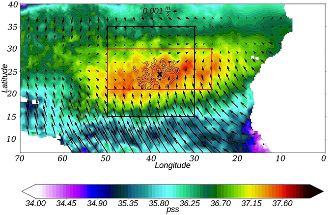
Figure 1. North Atlantic subtropical region, January 2013. Climatological monthly mean SSS from SMOS and Ekman velocity field using ERA-Interim. The black box indicates SPURS region. The red box is the region that was chosen for estimation of salinity budget. Black cross is the mooring position at 24.5°N 38°W.

To estimate a regional surface salinity budget during the period August 2012–2013, surface salinity product derived from the Soil Moisture and Ocean Salinity (SMOS) satellite mission, a regional ocean current product produced by AVISO and in situ data collected during the SPURS (Salinity Processes in the Upper-ocean Regional Study) experiment are used. The SPURS experiment took place in August 2012–April 2013 (Figure 1, black box). Its goal was to better understand the mechanisms responsible for salinity maximum formation in the subtropical North Atlantic (Oceanography special issue, 2015, Vol. 28, No. 1). The drifter data collected during SPURS and afterwards are used to validate the SMOS derived SSS and the ocean current products. The SST budget is estimated based on the OSTIA (Operational Sea Surface Temperature and Sea Ice Analysis) data. The SST budget is investigated to compare the meso-scale contribution in this budget to the one in the SSS budget, and better understand their effect on the SSS budget.

We will first describe the data sets and their accuracy in Section Data Sets and Validation before discussing the methodology in Section Method. Results and their discussion are then presented in Sections Results and Discussion and Summary respectively.

Data Sets and Validation

We investigate the area of 21°−30°N 50°−26°W. In the next section we will explain why we consider this region.

Spurs Drifters

The SPURS international experiment took place over one seasonal cycle during 2012/2013 (Figure 1, black box). Around 150 drifters were deployed in the central NSTG mostly in August–October 2012 and March–April 2013 (Centurioni et al., 2015). SVP-S drifters (Lumpkin and Pazos, 2007; Reverdin et al., 2007; Centurioni et al., 2015) have a battery pack, a satellite transmitter, a conductivity sensor below the surface float as well as a sea surface temperature (SST) sensor located either next to the conductivity cell or at the base of the float to avoid direct radiative heating. The drifters initially have a drogue centered at 15 m to follow the currents at this depth. Most of the drifters had a sensor to identify the presence of the drogue. In this work we use data of drogued SVP-S drifters. The time step of the data records is usually 30 min.

Mooring Data

The surface mooring was deployed as part of the SPURS project by the Upper Ocean Processes Group at WHOI at ~24.5°N 38°W (Figure 1, black cross). Data was collected from September 2012 until September 2013 by the ASIMET (Air-Sea Interaction Meteorology) system. The ASIMET system provides measurements of specific humidity, SST and conductivity, wind speed and direction, barometric pressure, shortwave radiation, longwave radiation, and precipitation. These variables are used to compute air-sea fluxes of heat, moisture and momentum using bulk flux algorithm. The accuracy of the mooring data is 8 Wm⁻² for the heat fluxes, 6 cm yr⁻¹ for the evaporation and 10% for precipitation (Colbo and Weller, 2009; Farrar et al., 2015). We use these mooring data to validate the gridded data sets of heat fluxes, evaporation and precipitation.

SMOS

The SMOS satellite mission was launched in November 2009 on a sun-synchronous circular orbit with a local equator crossing time at 6 a.m. on ascending node and at 6 p.m. on descending node. The SMOS mission carries an L-band (1.4 GHz) interferometric radiometer that allows the reconstruction of a bi-dimensional multi-angular image of the L-band brightness temperatures (Tb) that is used to retrieve the SSS (Kerr et al., 2010).

In the subtropical North Atlantic SMOS SSS suffers from a seasonally varying systematic error (Hernandez et al., 2014), especially strong during boreal winter (RMS close to 0.5, Figure 2). Systematic errors in SMOS SSS originate mainly from inaccuracies in instrument calibration, in image reconstruction (in particular the one that depends of the distance to coast, Kolodziejczyk et al., 2015a) and from anthropogenic RFI (Radio Frequency Interferences).

FIGURE 2

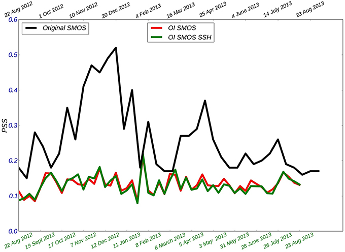
Figure 2. RMS differences at drifter positions (in pss) over the SPURS domain between drifters SSS and 10-day CEC-CATDS SMOS SSS product (black), SMOS-OI with (green) SSH or without (red) constraint.

In this work we use a new corrected and optimal interpolated (OI) SMOS SSS products described in Kolodziejczyk et al. (2015a,b, submitted), providing SSS to 75 km and 10 days resolution. The new OI SMOS SSS are derived from ESA level 2 SSS v550, using the same flagging as Boutin et al. (2013). The correction for systematic errors follows a two-step procedure: (1) removal of systematic errors in the vicinity to coast; (2) removal of seasonal systematic errors. First, data are corrected for 4-year mean (07/2010–07/2014) near coastal discrepancies with respect to the ISAS Argo climatology (Gaillard et al., 2009) taking into account that systematic errors depend on the location of the pixel across track and on the orbit orientation. Then, ascending and descending orbit data are mapped separately with an optimal interpolation scheme at large scale (500 km) with a Gaussian shaped correlation function. The seasonal large scale biases are then derived from the comparison with monthly ISAS SSS products. The last step is a noise reduction and mapping of bias corrected SMOS SSS every 7 days on the regular grid of 0.25° using optimal interpolation with a Gaussian correlation function scaled to 75 km over a window of 10 days centered on the day of mapping, using the corresponding monthly ISAS SSS fields as first guess.

In order to improve the horizontal SSS gradient at meso-scale, we also tested the introduction of a small constraint on along-stream-line (from AVISO SSH) orientation of the structures by including it in Gaussian correlation function (Kolodziejczyk et al., 2015a). This method allows to recover spatial scales slightly smaller than 75 km (OI SMOS SSH).

The SMOS OI (Figure 2, red curve) shows significant improvement with respect to earlier products (Figure 2, black curve, original SMOS product). The RMS difference between SMOS SSS at 10 days 75 km resolution and in situ data (TSGs, drifters) is lower than 0.15 almost for the whole period. The introduction of the supplementary correction (OI SMOS SSH) marginally, not significantly, improves the results (Figure 2, green curve). In this work we retained this last version of the weekly SMOS products with the spatial resolution of 0.25°.

As expected from the error statistics, the mapped (OI SSH) SMOS SSS field with the drifters' trajectories and data overlaid for the week 8–14 January 2013 (Figure 3) suggests that remaining systematic errors are small, and that the product captured a good part of meso-scale variability. Further discussions of the characteristics of the mapped product will be provided in another paper.

FIGURE 3

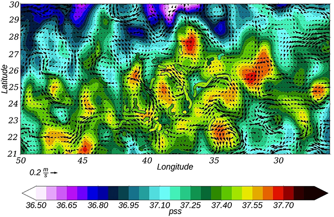
Figure 3. SMOS SSS vs. SPURS drifters and AVISO geostrophic velocity field, 8–14 January 2013.

From Figure 2 we just note that the error budget seems to remain relatively stationary in time. The small RMS error during August 2012 (Figure 2) results from a too small number of data for this period. There is a small peak of larger RMS difference in the week between January and February 2013 which could be due to a rain/wind front across this area inducing larger spatial variability and/or errors. Indeed, the rain front could have generated rapid and small scale wind changes not well captured in ECMWF (European Centre for Medium-Range Weather Forecasts) wind forecasts that are used in the SSS retrieval scheme.

Sea Surface Temperature OSTIA

To estimate the SST we use daily OSTIA SST analysis with horizontal resolution 0.05° (Reynolds and Chelton, 2010; Donlon et al., 2012). The SST product from OSTIA has zero mean bias and an accuracy of ~ 0.57 K compared to the in situ measurements as noted in Donlon et al. (2012).

AVISO Altimetry

A regional AVISO 2014 altimetric product (daily product with 1/8° spatial resolution) was chosen as the geostrophic velocity field (Dussurget et al., 2015, D15 product). Compared to the standard Ssalto-Duacs product, it uses less along-track filtering, which is optimized in this region and for the different satellites. It uses also an updated Mean Dynamic Topography (MDT). This product was validated with the drifter data. The ocean currents from this product fit reasonably well the drifter trajectories (example in Figure 3) and seem to be associated with deformations of the large scale SSS fields. Salinity gradients tend to align along the streamlines. For example, in the north of the area, there is a small advection of fresh water in salty region at 27°N 46°W that is explained by geostrophic AVISO currents. The eddies inside the high SSS area usually correspond to local SSS maxima or minima: 22°N 34°W, 23°N 30°W, or 26.5°N 44°W.

Argo Floats

We estimate MLD on individual Argo temperature-salinity profiles (Gould et al., 2004). The MLD is estimated, when a threshold value for either temperature or salinity is attained compared with a near-surface value at 10 m depth: ΔT = 0.1⁰C, ΔS = 0.03pss. We group these estimates monthly to provide a monthly mixed layer depth distribution (in the standard case, it is the average of the distribution that is retained). We use data from Coriolis web site with the flag “good data.” Because of insufficient data distribution, we only use them as providing a large scale average. The comparison (Figure 4) with the monthly gridded ISAS (In Situ Analysis System) fields (spatial resolution 0.5°), an optimal estimation tool designed for the synthesis of the Argo global data sets (Gaillard et al., 2009), at the Argo profile positions (blue curve) and averaged over the domain (green curve) shows a shallower MLD than the Argo data (red curve) throughout the year, with the maximum difference of ~25 m in December. The interpolation of Argo data can smooth the local MLD deepening, especially in December when there are more local rain events in this region. The consideration of the MLD in different latitude bands (Figure 4, red dashed curves) shows a horizontal gradient (from shallower MLD in the South to deeper in the North) and different restratification time (March in southern regions and March-April in northern regions; Kolodziejczyk et al., 2015c).

FIGURE 4

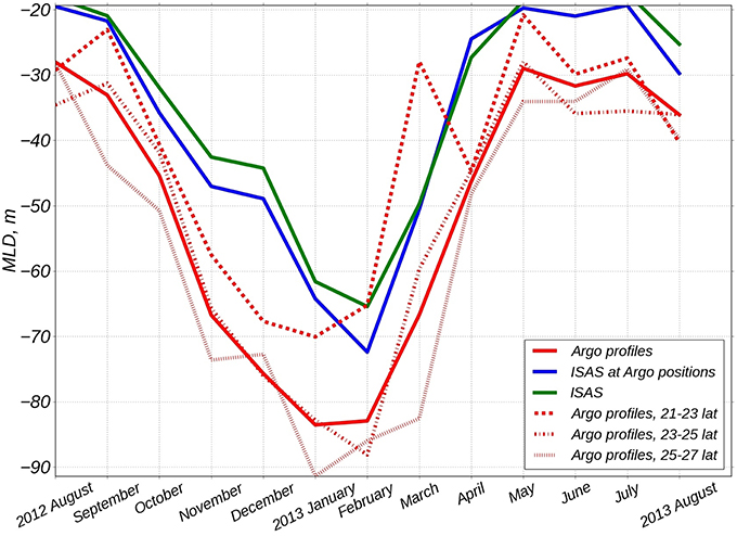
Figure 4. MLD from Argo (red) and ISAS interpolated product (blue and green) for period August 2012—August 2013. MLD from Argo profiles for different latitude bands (red dashed lines).

Atmospheric Fluxes

Freshwater Flux

Daily Era-Interim reanalysis from ECMWF (spatial resolution 0.25° × 0.25°), widely used daily OAFlux product (1° × 1°) from Woods Hole Oceanographic Institution (WHOI) for evaporation field and daily Era-Interim reanalysis, TRMM TMI (3B42) (0.25° × 0.25°) and GPCP (1° × 1°) satellites for precipitation field were tested. GPCP is strongly based on satellite retrievals, such as TRMM TMI, and surface rain gauges (Adler et al., 2012).

The comparison of evaporation field from Era-Interim (Figure 5A), black curve) with ones from OAFlux (Figure 5A), blue curve) indicates small differences between ~0 and 0.5 mm/day. The comparison with the mooring data at 24.5°N 38°W (see 2.2, Figure 5A), low-passed filtered data with 30 days cut-off) shows that ERA-Interim product sometimes (October, November, June) overestimates evaporation (max ~0.5 mm/day) but usually in the confidence interval from the mooring data (0.16 mm/day) with a high correlation, while OAFlux product underestimates a little (max ~0.7 mm/day and it is out of the mooring confidence interval in spring and summer) evaporation during almost the whole period. This is in line with the expectation that OAFlux might slightly underestimate the evaporation (from ERA-Interim and buoys) in the subtropical gyre of the North Atlantic (Yu et al., 2008).

FIGURE 5

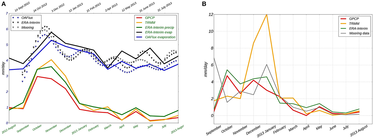
Figure 5. (A) —Evaporation (ERA-Interim—black curve, OAFlux—blue) and precipitation (GPCP—red, TRMM—orange, ERA-Interim—green) data averaged over the month and over the domain (solid lines) and evaporation filtered with cut-off period 30 days at mooring position 24.5°N 38°W (dashed lines, mooring data—gray curve); (B) —precipitation data at mooring position.

On the other hand, Era-Interim reanalysis produces larger precipitation events over the North Atlantic compared with the satellite data (Figure 5A), green curve). TRMM satellite precipitation (Figure 5A), orange curve) is stronger than one from GPCP (Figure 5A), red curve) (Huffman et al., 2001). The comparison with the mooring data does not show a good agreement between the different products, even after monthly averaging (Figure 5B). ERA-Interim shows much higher total precipitation (2.58 mm/day) compared with mooring data (1.86 mm/day ± 10%), TRMM overestimates high precipitation events (total precipitation 2.76 mm/day). GPCP does not correlate well with the mooring time series, but presents a very close total precipitation average (1.69 mm/day). We retain GPCP in this work.

Heat Fluxes

The latent heat, sensible heat, net downward short and long wave radiations from ERA-Interim with the resolution 0.25° × 0.25° are used to estimate the surface heat flux. ERA-Interim net surface heat flux presents a satisfactory agreement with the one from mooring data at 24.5°N 38°W (Figure 6). The average over the year for the incoming short wave radiation is 220.3 Wm⁻² with mooring data and the net downward short wave radiation is 252.06 Wm⁻² with ERA-Interim, for the long wave radiation it is respectively −58.84 W/m² and −58.9 Wm⁻², for the sensible heat flux it is respectively −6.37 Wm⁻² and -13.19 Wm⁻², and for the latent heat flux it is −124.08 Wm⁻² and −144.37 Wm⁻² respectively, so that the net heat flux across the sea surface of the two products differ by less than 6 Wm⁻².

FIGURE 6

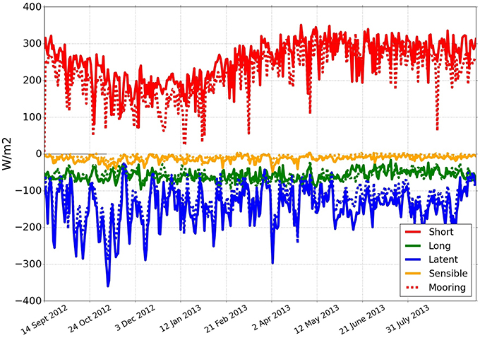
Figure 6. Surface heat flux for the period September 2012–August 2013; solid curves—ERA-Interim reanalysis, dashed curves—mooring data at 24.5°N 38°W, red—net short wave radiation, green—net long wave radiation, blue—latent heat, orange—sensible heat.

Method

We consider the ML salinity (MLS) budget that can be written as (based on the conservation equation of any tracer with additional scale separation) (Delcroix and Hénin, 1991):

$\begin{array}{cc}\begin{array}{l}\frac{\partial \langle S\rangle }{\partial t}=-\langle u^{\prime }\nabla S^{\prime }\rangle -\langle \overline{u}\nabla \overline{S}\rangle -\frac{(S_{10m}-S_{-entr})}{h}\left(\frac{\partial h}{\partial t}+\langle w_{-h}\rangle \right)\\ +\langle \frac{(E-P)S}{h}\rangle +\text{R},\end{array}& \left(1\right)\end{array}$

where <S> denotes SSS averaged over the domain for each time step (month), S is the mean salinity over a 90 days period for each grid point, u = ū + u′, h is MLD averaged over domain, w_−h is the Ekman vertical velocity calculated with the Era-Interim wind, u is the horizontal velocity vector, the sum of geostrophic AVISO velocity field and Ekman velocity that was calculated as $\frac{\overrightarrow{\tau }}{\rho fh}$, (E-P) is the difference between evaporation and precipitation. In term of entrainment S_10m is the salinity at 10 m depth (that is considered as the salinity of MLD), S_−entr is the salinity of the entrained water and is estimated as the salinity at the depth $\left(\frac{\partial h}{\partial t}+w_{-h}\right)\times \Delta T$, (with ΔT = 1month ≈ 2592000s) that scales the layer of entrained water during the month considered (a month is the elementary time step in the mixed layer depth analysis). The left side of the equation presents the MLS tendency. The first term of the right side of the equation is turbulent horizontal advection estimated at each grid point and then monthly averaged over domain; the second one is mean horizontal advection estimated as the previous term. The third term presents the entrainment component (here we used Argo profile salinity, and neglect horizontal gradients when estimating this term as the MLD was chosen the same over whole domain for the considered month). The fourth term is the surface forcing that was estimated in the same manner as advection terms. The last one R is residual term that includes the sum of all unresolved physical processes and the accumulated errors from the other terms.

Similarly, the ML temperature (MLT) budget can be written as Moisan and Niiler (1998):

$\begin{array}{cc}\begin{array}{l}\frac{\partial \langle T\rangle }{\partial t}=-\langle u^{\prime }\nabla T^{\prime }\rangle -\langle \overline{u}\nabla \overline{T}\rangle -\frac{(T_{10m}-T_{-entr})}{h}\left(\frac{\partial h}{\partial t}+\langle w_{-h}\rangle \right)\\ +\langle \frac{(Q)}{\rho C_{p}h}\rangle +\text{R},\end{array}& \left(2\right)\end{array}$

where <T> is SST averaged over the domain for each time step (month), Q is the surface heat flux, C_−p is the specific heat capacity, ρ is density, all other terms are the same as for salinity budget. The surface heat flux can be calculated as Q = Q_l + Q_s + Q_lw + (1 − α)Q_sw[1 − I(h)] (Morel and Antoine, 1994; Sweeney et al., 2005), where Q_l is latent heat, Q_s is sensible heat, Q_lw is net long wave radiation, Q_sw is net short wave radiation, α = 0.04 is the ocean surface albedo, $I(h)=R{e}^{-h∕D_1}+\left(1-R\right)e^{-h∕D_2}$ is the penetrative solar irradiance with the fraction of total solar flux for wavelengths longer than 700 nm R = 0.58, it is assumed to penetrate the ocean with a decreasing exponential profile, with an e-folding depth scale D₁ = 0.35m; D₂ = 23m is the second extinction length scale associated with the shorter wavelength (Madec and the NEMO team, 2014).

All data sets were interpolated to the OI SMOS grid with the spatial resolution 0.25 × 0.25°. The error bars for each term were estimated by propagating the errors on the data (Appendix B in Supplementary Material).

We chose the region within the latitudes/longitudes range 21°−30°N/50°−26°W in subtropical Atlantic salinity maximum. It encompasses the region of largest SSS and strong SSS horizontal gradients just out of the domain (Figure 7A). In particular in the south one expects the strong SSS gradient due to a very large contribution from Ekman currents. Moreover, there is a large eddy variability in the North and in the West where the annual mean of SSS variability $\frac{\partial \langle S\rangle }{\partial t}$ reaches more than 0.6 pss/yr which is two times higher than in the center of the box (Figure 7; on the southern and eastern boundaries we are limited by the availability of the regional AVISO data). On Figure 7B (the annual mean of the turbulent salinity advection) the strong effect of eddy variability is further north, south and west (out of the domain), where it shows higher maximum absolute value larger than 0.6 pss/yr almost everywhere for these regions. On Figure 7C (the annual mean of the mean salinity advection) one notes the strong effect of Ekman currents further north and south up to 0.75 pss/yr. Furthermore, the spatial concentration of drifters and Argo data is larger in the center of the region and used to check the realism of the analysis.

FIGURE 7

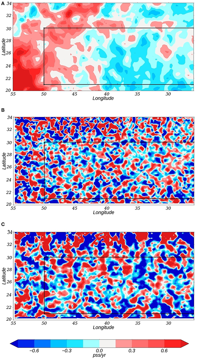
Figure 7. Terms of the Equation (1) averaged over the year August 2012—August 2013; (A) —time salinity change, (B) —turbulent advection term, (C) —mean advection term.

Results

Salinity Budget

As mentioned before, SSS maximum is located a few degrees to the north of the E-P maxima (Figure 8) which shows the importance of the ocean dynamics in this region (Qu et al., 2011), indicating in particular a contribution of Ekman advection, and suggesting a large scale balance between sea surface forcing, advection and mixing processes. In winter 2012–2013 (especially in December) a rain band was found in the middle of the region which resulted in two local maxima on Figure 8B.

FIGURE 8

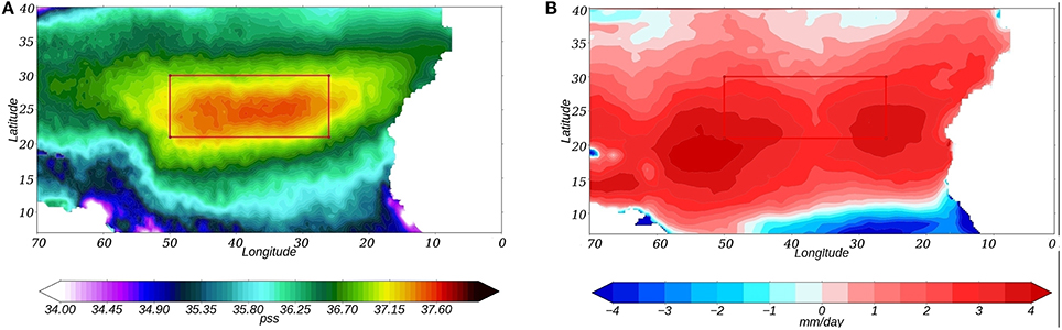
Figure 8. Annual salinity (A) and E-P (B) mean with the selected region for SSS budget estimation (red box) over the August 2012—August 2013.

The terms in Equation (1) were estimated and averaged over the whole domain (Figure 9A). As expected, there is a strong response of the surface ocean to the evaporation flux (blue curve) on the salinity change term (green curve). The error bar is large during autumn and early winter months. This is due to local precipitation events and fast temperature changes, as consequences the evaporation changes that are not well reproduced.

FIGURE 9

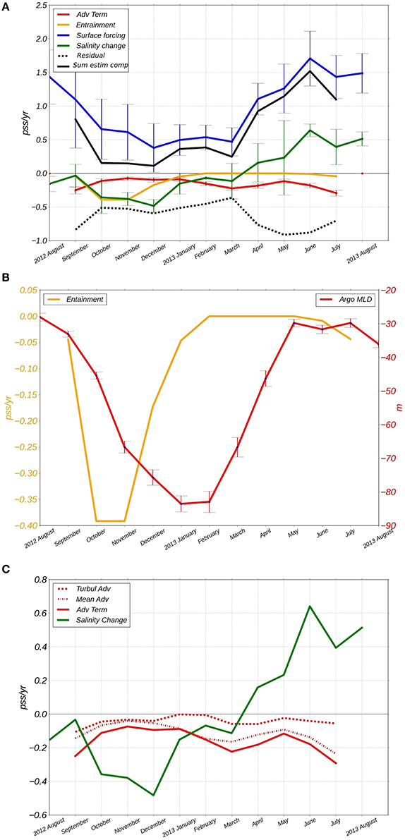
Figure 9. (A) —components of salinity budget, residual (black dashed curve) and the sum of all estimated components of the right side of the Equation (1) (black curved); (B) —entrainment (orange curve) and Argo MLD (red); (C) —salinity change (green) and advection components (red).

The entrainment term contributes only during autumn and winter months when MLD is deepening (Figures 9A,B), orange curve). During the winter months entrainment plays a smaller role as the deepening of the ML is weaker and the MLS is closer to the salinity that is found deeper (S_−entr). In November when there is a small increase in the surface forcing term (evaporation increases) salinity continues to lower due to entrainment. In December, a month with larger amount of precipitation and small entrainment, the salinity changes are predominantly governed by surface freshwater flux (Figure 9A). Due to the difficulty in estimating the error on entrainment, only the error bars (standard error) on MLD is shown (Figure 9B).

For the whole domain the spatially averaged advection is negative throughout the year with a relatively small amplitude (Figures 9A,C). The turbulent and mean advections are both negative with the stronger magnitude for the mean component. It shows a moderate seasonal cycle associated with a maximum freshening during summer.

The sum of all estimated equation's component in the right side of the Equation (1) (here and after does not include R) (Figure 9A), black curve is very close to the surface forcing term and its difference with $\frac{\partial \langle S\rangle }{\partial t}$ gives a large residual term R (Figure 9A), black dashed curve.

To better understand the effect of advection we separate the region into two boxes: 21°−25.5°N 50°−26°W and 25.5°−30°N 50°−26°W. The dividing latitude was chosen based on the seasonal means and seasonal variability maps of the equation's terms (Figure 10). During the winter, the SSS variability term (Figure 10A) is characterized by salinity decreases north of 25.5°N, while a region with variable salinity changes (salinity can increase as well as decrease) is found in the South. For the SSS variability in the summer season (Figure 10B) the latitude 25.5°N separates a region of dominant increase in the North from a dominant decrease in the South. It means that during the summer the strong increase of SSS takes place in the northern region, while during the winter there is the largest decrease. Autumn and spring (not presented) show similar patterns for these two regions. The advection variability maps (Figures 10C,D) show two different structures in the southern part. During autumn (Figure 10C) some freshwater originating from the Amazon basin enters this region and is mixed through the domain, inducing a strong variation of turbulent advection in the south-western part (the std is up to 10 pss/yr in this region). During spring (Figure 10D) mean advection plays a significant role in the salinity change with significant spatial variability both in the northern as well as in the southern parts. Surface water flux (Figures 10E–G) shows strong spatial variability in both regions during the autumn (Figure 10E) and in the South during the spring (Figure 10F) when evaporation largely dominates there. The mean surface forcing (Figure 10G) also exhibits different regime on either side of 25.5°N that isolate the southern region, the region of maximum E-P field. Thus, 25.5°N separates two regimes in the SSS budget variability in agreement with Dong et al. (2015).

FIGURE 10

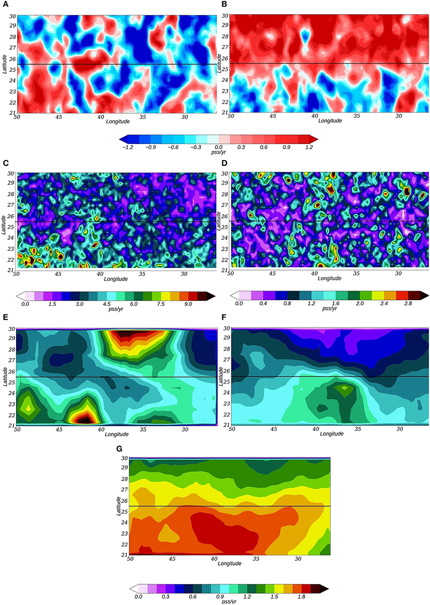
Figure 10. Sea surface salinity change in winter (A) and summer (B). Turbulent advection standard deviation in autumn (C) and mean advection standard deviation in spring (D). Surface forcing standard deviation in autumn (E) and spring (F) and surface forcing mean in summer (G).

In the southern part, both the turbulent advection and mean advection (Figure 11A) play a significant role during the autumn and brings fresh water through eddy transport. On the other hand, during spring and summer it is rather the mean advection that brings freshwater from the tropical regions. In the northern part (Figure 11B), advection does not show significant variability throughout the year except during summer when mean advection brings the salty water from the south and contributes to the salinity increase. In general, the domain-averaged salinity presents large month-to-month changes throughout the year (intraseasonal variability) in the southern part (Figure 11C) and seasonal cycle in salinity in the northern part (it decreases in winter and increases in summer). In the southern part, SSS decreases until October due to the small surface forcing, the effect of the advection and the entrainment terms. Afterwards there is a salinity increase in November. At this time the surface flux continues to decrease and the advection terms diminish in absolute value and reduces its freshening effect on the salinity. At that time even strong entrainment cannot significantly refresh the surface water. In December the salinity again decreases while freshwater flux increases, the entrainment starts to be smaller and there is only a small decrease in advection term that cannot match this strong change in salinity. Thus, in this month other processes contributing to the much larger residual term probably increase.

FIGURE 11

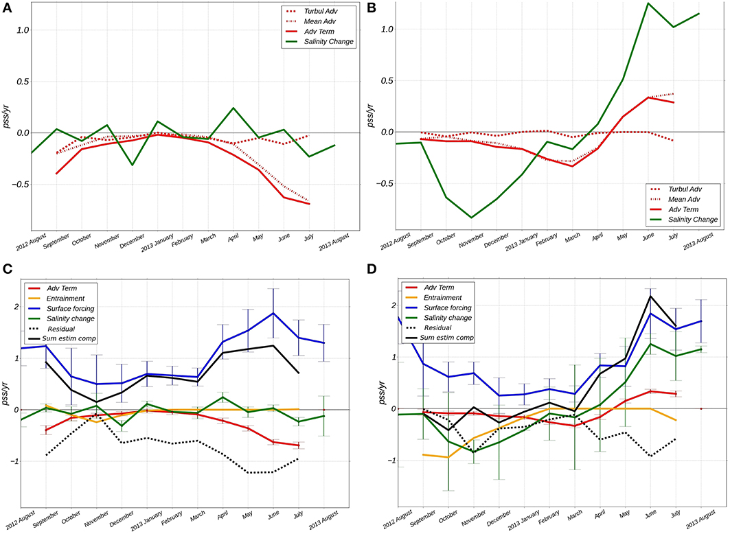
Figure 11. Salinity change (green) and advection components (red) (A,B) and components of salinity budget, residuals (black dashed curves) and sums of right side's estimated equation components (C,D), Equation (1). (A,C) −21°−25°N, (B,D) −25°−30°N.

During the summer months, the salinity change is controlled by advection associated with transport of fresher water from the tropics that partially counterbalances the gain from evaporation. In the northern domain (Figure 11D) during winter the salinity change is strongly influenced by entrainment of deeper water and horizontal advection that contribute to a decrease of SSS. One of the two local minima of the residual component is found at this time.

In summer, the salinity increase strongly depends on advection which brings salty water from the E-P maxima region, and freshwater flux which concomitantly increases. The residual terms are large and in the range from 0 to −1.5 pss/yr in particular for the southern region.

Heat Budget

The estimation of the temperature budget based on Equation (2) in the subtropical gyre of the North Atlantic (Figure 12) indicates a near-balance between the terms retained, i.e., the error bar range of the two sides of the equation overlap [black solid (the sum of all elements in the right part of the Equation (2)] and green (temperature change) curves). The different components of the temperature budget have the same pattern irrespective of the domain [total region (Figure 12A), southern (B) and northern (C) parts]. SST (green curve) decreases in late autumn and winter and increases in spring and summer. The term of surface heat flux (blue curve) shows comparable variability in the two regions being largely responsible for the temperature change. The entrainment term (orange curve) is large during late autumn and winter and contributes to lower SST. Only the terms of horizontal advection are different for the southern (Figure 12B) and the northern (Figure 12C) parts. In the southern part, advection is negative throughout most of the year, bringing colder water mostly from the North, whereas it is positive during spring and late summer, the period of large warming. In the northern part the sign of advection is the same, except for November and December with a positive advection term. It implies that during these 2 months the horizontal gradient of SST was small over the region. After this period the colder water comes from the North and the East, resulting in negative advection terms. As commented the net residual terms are relatively small with an annual negative average.

FIGURE 12

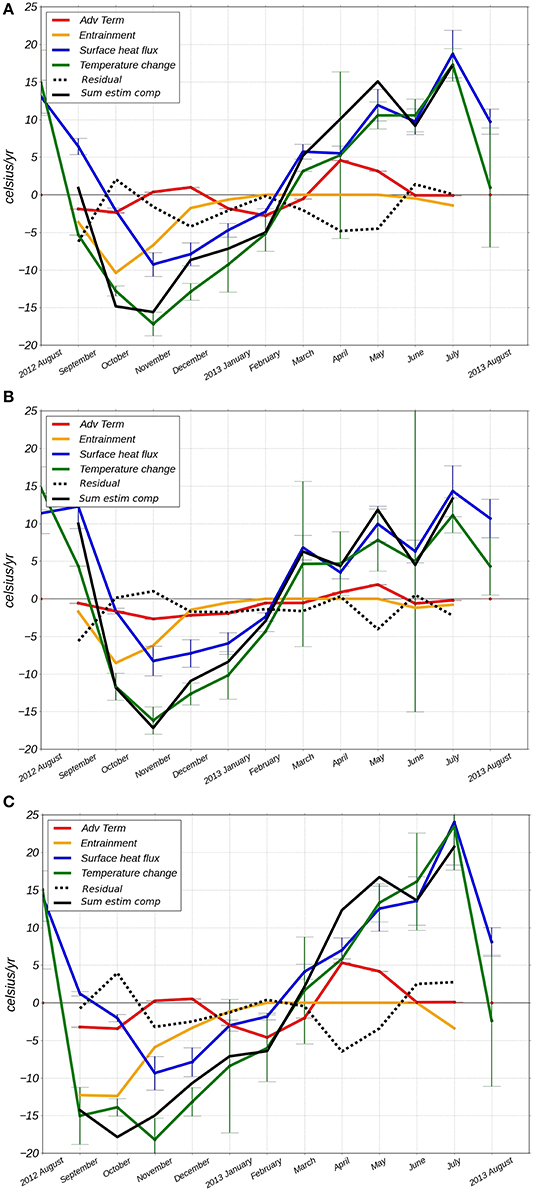
Figure 12. Components of temperature budget for the period August 2012–2013, residual (black dashed curves) and the sum of all estimated components of the right side of the Equation (2). (A) —total considered region; (B) —southern part 21°–25°N; (C) —northern part 25°−30°N.

Discussion and Summary

We examined the salinity and temperature budgets in the subtropical gyre of the North Atlantic 21°-30°N/50°-26°W during the period August 2012–2013 based on the OSTIA data for SST and CATDS CEC LOCEAN SMOS corrected data (OI SMOS and OI SMOS SSH) for the SSS. The OI SMOS SSS gives promising results, as a comparison with drifter data shows RMS differences on the order of 0.15 even in winter; the introduction of a constraint coming from SSH marginally improves the results. The spatially-averaged SSS presents a realistic seasonal cycle with the minimum in winter and maximum in summer (Figure 9A), as is also found for SST (Figure 12). This region contains an Ekman convergence zone around 25.5°N which results in two different regimes within the box. The division of the region into two parts shows that in the southern part of the domain SSS does not present a seasonal cycle. In this region the freshwater flux is partially balanced by other terms of the salinity budget while in the northern region the effect of the freshwater flux is dominant. The SST budget presents a similar variability in the southern and northern parts. The gradient of SST changes sign on the diagonal (from South-West to North-East) of the box compared with the meridional gradient of the SSS. The effect of warm water from the equator is first felt in the southern part during early spring with an earlier and faster increase of SST than in the northern domain.

The freshwater flux is the dominant component in the salinity budget (0.88 ± 0.3 pss/yr, averaged over the period September 2012 – July 2013 and over 21°−30°N/50°−26°W region) while the heat flux (2.9 ± 1.34 C°/year; for the 13 month period it is 4.12 ± 1.43 C°/year) is the dominant component in the temperature budget. Both of them have a seasonal cycle with a minimum in winter and maximum in summer. The heat flux is responsible for the variability in SST throughout the year. SSS and SST do not show a strong tendency 0.014 ± 0.2 pss/yr and 1.5 C°/yr over these 11 months, similar to the results averaged over the 10-years (2004–2013) period and over the SPURS-1 region in Dong et al. (2015) (for salinity). Dong et al. (2015) have found a 1-month lag between the salinity change and the seasonal cycles of surface forcing term, which might be the result of a slightly different region retained in their analysis [notice that Dong et al. (2015) domain is 5° further south than the region in Figure 1 (red box)].

The advection term depends on the scale, region and time period. Farrar et al. (2015) shows the strong influence of advection at the meso-scale, whereas in Dohan et al. (2015) the large-scale advection term is small compared with the amplitude of the sea surface forcing and is referred to as “residual term.” Dong et al. (2015) have shown that the Ekman and geostrophic advection mean state component nearly compensate each other in the region 20°−30°N 45°−30°W. In the region that we retained we find that the advection term (Figure 9A, red curve) does not present a large seasonal variability and contributes to a negative (freshening) effect on the total budget (−0.16 ± 0.02 pss/yr in our work to be compared with Dong et al. (2015) −0.28±0.01 pss/yr for the period 2004–2013 and over the larger region). The mean part of the advection term plays a dominant role in the salinity budget in the subtropical gyre of the North Atlantic (the mean part equals −0.11±0.02 pss/yr whereas the turbulent part equals −0.04±0.02 pss/yr). In the two sub-regions the role of the advection terms starts to be clearer: (1) the effect of the turbulent advection component is important in the southern part during the autumn when it contributes to a freshening; (2) in spring and summer Ekman advection brings fresher water from the equatorial zone to the southern part of the domain, whereas its salty water from the E-P maximum region is transferred further North where it contributes to the salinity increase; thus it explains the strong contribution of mean component in the southern region, −0.18±0.04 pss/year and −0.06±0.04 pss/year for the turbulent component. In the temperature budget the value of the averaged advection term over the period and domain plays a small negative (cooling) role (−0.04±0.02 C°/yr) as the values of the mean and turbulent advections are −0.16±0.02 C°/yr and 0.12 ± 0.02 C°/yr, respectively. This suggests that the turbulent advection has a strong positive effect (warming) than mean advection but the turbulent component is still small compared with the other terms while the mean term varies throughout the year which “compensate” when averaged over the year (not shown).

The entrainment component plays a role during autumn and winter when mixed layer deepens. In the salinity budget this term has a modest effect (−0.15 pss/yr) while in the temperature budget it is the major component that compensates the effect of the heat flux (−3.58 C°/yr).

Despite the physical consistency of the results, the salinity budget cannot be closed. The surface forcing term has a strong influence on the salinity and temperature budgets. Errors on this term induce errors in the salinity budget estimation as suggested by the fact that the residual terms (Figures 9A, 11C,D, 12) tend to mirror the freshwater flux terms. Furthermore, the error bar on freshwater flux (resulting from time-space variability) exceeds 0.6 pss/yr in autumn and spring/summer seasons, the periods where the residual term is large. In the autumn, there is also the possibility that the precipitation might not be correctly estimated, whereas in the summer months, the comparison with the mooring data suggested a possible overestimation of evaporation in the ERA-Interim reanalysis used here.

The error bars on advection terms are small but in some region the AVISO product underestimates the geostrophic velocity (comparison with surface drogued drifters, unpublished results). This later effect could change our results a little but probably not significantly as the results for the temperature budget (Figure 12) with the same data sets show a much closer budget. There is however also for that term the possibility that the SMOS-product that we used presents too large errors or smooths out some of the scales responsible for the meso-scale advection (but see Appendix A in Supplementary Material, which suggests that at least at 0-order it produces a reasonable estimate).

The errors are also sensitive to the MLD chosen. In order to estimate entrainment we use the MLD averaged over the domain. This approach excludes the consideration of the horizontal gradient, and salinity change by induction which may be not negligible in the area (see for example Dohan et al., 2015; Dong et al., 2015). This contributes to uncertainties in our results, and obviously misses more local and smaller scale processes. At this point the data used do not allow to evaluate the effect of a spatial change in MLD at meso-scale. But the fact that this method gives good results for SST budget means that the SSS is more sensitive to the vertical processes such as restratification, mixing and etc.

Altogether we find large residuals from the salinity budget ~−0.3 pss/yr (or 47% of the average modulus of $\frac{\partial \langle S\rangle }{\partial t}$ which varies in the range ±0.63 pss/yr), whereas they are much smaller for the temperature budget, also with a negative average, −0.77 C°/yr (~4% of the average magnitude of $\frac{\partial \langle T\rangle }{\partial t}$ which varies in the range ±18 C°/yr) (see Table 1). It is probably due to the strongest effect of the heat flux on the temperature change that simplifies the estimation of temperature budget, while the salinity variability strongly depends on the ocean dynamics (Figure 8). The advection is the most important component for the salinity budget in this region and can be the main source of errors due to the uncertainties in salinity field and underestimation of velocity field that was discussed above. Moreover it is thus difficult to blame a choice of a too shallow mixed layer in the summer months, as it would contribute to a negative residual in the SSS budget, but also in the SST budget. Small scale processes such as are found near filaments or fronts, could be a source of asymmetry between the SST and SSS budgets. Indeed, in the southern part of the domain, Kolodziejczyk et al. (2015c) showed that SSS spatial variability dominates the surface density gradients. This was also witnessed in summer during the Strasse cruise (Reverdin et al., 2015), and in early spring during the Midas cruise (Busecke et al., 2014). Dynamical processes that induce mixed layer restratification would thus contribute to an average SSS decrease, but with little notable effect on SST (Shcherbina et al., 2015). In addition, vertical mixing with salt fingering at the lower boundary of the mixed layer would also contribute to a larger SSS negative term compared with SST, but this would happen preferentially when there is a large salinity vertical stratification compared to temperature, and thus probably not in the summer months. In some studies the mismatch (residual) is parameterized by eddy horizontal diffusion terms, as in Dong et al. (2015) when such a term contributes to the MLS changes with the averaged magnitude of −0.28±0.01 pss/yr thus comparable with our residual term (−0.3 pss/yr).

TABLE 1

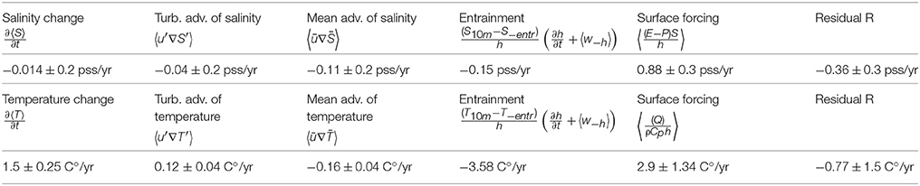
Table 1. Annual averaged means of the components in Equations (1) and (2).

Using other data sets (for precipitation, evaporation, MLD, etc.) to estimate the salinity budget could help better understand the mechanism of formation of the salinity maximum of the subtropical North Atlantic and its seasonal variability. Further testing other ways to estimate entrainment or a relevant mixed layer depth would also improve the reliability of these results. In further work we will also estimate the SSS and SST budget based on Mercator PSY2V4R4 simulation data to improve the entrainment estimation method, to validate the model data on the meso-scale and to estimate subscale horizontal diffusion and impact of vertical processes.

Author Contributions

AS has done the analysis of the budgets of surface temperature and salinity in the North Atlantic subtropical gyre during SPURS experiment. GR is the Thesis supervisor of AS. He tested the salinity drifters and contributed to their operation during SPURS. He is the French PI in SPURS experiment. NK has characterized meso-scale variability in surface salinity from SMOS band-L radiometer remote sensing data. JB is the specialist on band-L radiometry data and a SMOS-mission French PI. She also contributed to the supervision of AS.

Conflict of Interest Statement

The authors declare that the research was conducted in the absence of any commercial or financial relationships that could be construed as a potential conflict of interest.

Acknowledgments

The authors thank the two reviewers for their helpful comments. The authors thank the CLS team who work on the regional AVISO altimetry product: R. Dussurget, S. Mulet, M.-I. Pujol, M.-H. Rio. The original altimeter products were produced by Ssalto/Duacs and distributed by AVISO, with support from CNES (http://www.aviso.altimetry.fr/duac). SVP drifters were provided by the Global Drifter Program, NOAA grant #NA10OAR432056. LC and VH were supported by NASA grant #NNX12AI67G and NOAA grant #NA10OAR432056. This work was carried out in the frame of the SMOS-Ocean CNES/TOSCA project. The study was also supported in France by two grants of LEFE/IMAGO and LEFE/GMMC. A. Sommer is co-founded by CNES and UPMC PhD fellowships.

Supplementary Material

The Supplementary Material for this article can be found online at: https://www.frontiersin.org/article/10.3389/fmars.2015.00107

References

Adler, R. F., Gu, G., and Huffman, G. J. (2012). Estimating climatological bias errors for the global precipitation climatology project (GPCP). J. Appl. Meteor. Climatol. 51, 84–99. doi: 10.1175/JAMC-D-11-052.1

CrossRef Full Text | Google Scholar

Boutin, J., Martin, N., Reverdin, G., Yin, X., and Gaillard, F. (2013). Seas surface freshening inferred from SMOS and Argo salinity: impact of rain. Ocean Sci. 9, 183–192. doi: 10.5194/os-9-183-2013

CrossRef Full Text | Google Scholar

Busecke, J., Gordon, A. L., Li, Z., Bingham, F. M., and Font, J. (2014). Subtropical surface layer salinity budget and the role of mesoscale turbulence. J. Geophys. Res. Oceans 119, 4124–4140. doi: 10.1002/2013JC009715

CrossRef Full Text | Google Scholar

Centurioni, L. R., Hormann, V., Chao, Y., Reverdin, G., Font, J., and Lee, D. K. (2015). Sea surface salinity observations with Lagrangian drifters in the tropical North Atlantic during SPURS: Circulation, fluxes, and comparisons with remotely sensed salinity from Aquarius. Oceanography 28, 96–105. doi: 10.5670/oceanog.2015.08

CrossRef Full Text | Google Scholar

Colbo, K., and Weller, R. A. (2009). Accuracy of the IMET sensor package in the subtropics. J. Atmos. Oceanic Technol. 26, 1867–1890. doi: 10.1175/2009JTECHO667.1

CrossRef Full Text | Google Scholar

Dai, A., Qian, T., Trenberth, K. E., and Milliman, J. D. (2009). Changes in continental freshwater discharge from 1948 to 2004. J. Clim. 22, 2773–2792. doi: 10.1175/2008JCLI2592.1

CrossRef Full Text | Google Scholar

Delcroix, T., and Hénin, C. (1991). Seasonal and interannual variations of sea surface salinity in the tropical Pacific Ocean. J. Geophys. Res. 96, 22135–22150. doi: 10.1029/91JC02124

CrossRef Full Text | Google Scholar

Dohan, K., Kao, H.-Y., and Lagerloef, G. S. E. (2015). The freshwater balance over the North Atlantic SPUS domain from aquarius satellite salinity, OSCAR satellite surface currents, and some simplified approaches. Oceanography 28, 86–95. doi: 10.5670/oceanog.2015.07

CrossRef Full Text

Dong, S., Goni, G., and Lumpkin, R. (2015). Mixed-layer salinity budget in the SPURS region on seasonal to interannual time scales. Oceanography 28, 78–85. doi: 10.5670/oceanog.2015.05

CrossRef Full Text

Donlon, C. J., Martin, M., Stark, J. D., Roberts-Jones, J., Fiedler, E., and Wimmer, W. (2012). The operational sea surface temperature and sea ice analysis (OSTIA). Rem. Sens. Environ. 116, 140–158. doi: 10.1016/j.rse.2010.10.017

CrossRef Full Text | Google Scholar

Durack, P. J. (2015). Ocean salinity and the global water cycle. Oceanography 28, 20–31. doi: 10.5670/oceanog.2015.03

CrossRef Full Text | Google Scholar

Durack, P. J., and Wijffels, S. E. (2010). Fifty-years in Global ocean salinities and their relationship to broad-scale warming. J. Clim. 23, 4342–4362. doi: 10.1175/2010JCLI3377.1

CrossRef Full Text | Google Scholar

Dussurget, R., Mulet, S., Pujol, M.-J., Sommer, A., Kolodziejczyk, N., Reverdin, G., et al. (2015). Surface current field improvements – Regional altimetry for SPURS. Coriolis Mercator Newslet. 52, 39–44.

Farrar, J. T., Rainville, L., Plueddemann, A. J., Kessler, W. S., Lee, C., Hodges, B. A., et al. (2015). Salinity and temperature balances at the SPURS central mooring during fall and winter. Oceanography 28, 56–65. doi: 10.5670/oceanog.2015.06

CrossRef Full Text | Google Scholar

Gaillard, F., Autret, E., Thierry, V., Galaup, P., Coatanoan, C., and Loubrieu, T. (2009). Quality control of large Argo data sets. J. Atmos. Oceanic Technol. 26, 337–351. doi: 10.1175/2008JTECHO552.1

CrossRef Full Text | Google Scholar

Gordon, A. L., and Giulivi, C. F. (2014). Ocean eddy freshwater flux convergence into the North Atlantic subtropics. J. Geophys. Res. Oceans 119, 3327–3335. doi: 10.1002/2013JC009596

CrossRef Full Text | Google Scholar

Gould, J., Roemmich, D., Wijffels, S., Freeland, H., Ignaszewsky, N., Jianping, X., et al. (2004). Argo profiling floats bring new era of in situ ocean observations. Eos Trans. Am. Geophys. Union. 85, 185–191. doi: 10.1029/2004EO190002

CrossRef Full Text | Google Scholar

Hasson, A., Delcroix, T., and Boutin, J. (2013). Formation and variability of the South Pacific Surface Salinity maximum in recent decades. J. Geophys. Res. 118, 5109–5116. doi: 10.1002/jgrc.20367

CrossRef Full Text | Google Scholar

Hernandez, O., Boutin, J., Kolodziejczyk, N., Reverdin, G., Martin, N., Gaillard, F., et al. (2014). SMOS salinity in the subtropical North Atlantic salinity maximum: Part 1. Comparison with Aquarius and in situ salinity. J. Geophys. Res. Oceans 119, 8878–8896. doi: 10.1002/2013JC009610

CrossRef Full Text | Google Scholar

Huffman, G. J., Adler, R. F., Morrissey, M., Bolvin, D. T., Curtis, S., Joyce, R., et al. (2001). Global precipitation at one-degree daily resolution from multi-satellite observations. J. Hydrometeor. 2, 36–50. doi: 10.1175/1525-7541(2001)002<0036:GPAODD>2.0.CO;2

CrossRef Full Text | Google Scholar

Kerr, Y. H., Waldteufel, P., Wigneron, J.-P., Delwart, S., Cabot, F., Boutin, J., et al. (2010). The SMOS mission: new tool for monitoring key elements of the global water cycle. Proc. IEEE 98, 666–687. doi: 10.1109/JPROC.2010.2043032

CrossRef Full Text | Google Scholar

Kolodziejczyk, N., Boutin, J., Hernandez, O., Sommer, A., Reverdin, G., Marchand, S., et al. (2015a). Argo SSS and SMOS SSS combination helps monitoring SSS variability from basin scale to mesoscale. Coriolis Mercator Newslett. 52, 16–21.

Google Scholar

Kolodziejczyk, N., and Gaillard, F. (2013). Variability of the heat and salt budget in the subtropical southeastern pacific mixed layer between 2004 and 2010: spice injection mechanism. J. Phys. Oceanogr. 43, 1880–1898. doi: 10.1175/JPO-D-13-04.1

CrossRef Full Text | Google Scholar

Kolodziejczyk, N., Hernandez, O., Boutin, J., and Reverdin, G. (2015b). SMOS salinity in the subtropical North Atlantic salinity maximum: 2. Two-dimensional horizontal thermohaline variability. J. Geophys. Res. Oceans 120, 972–987. doi: 10.1002/2014JC010103

CrossRef Full Text | Google Scholar

Kolodziejczyk, N., Reverdin, G., and Lazar, A. (2015c). Interannual variability of the mixed layer winter convection and spice injection in the eastern subtropical North Atlantic. J. Phys. Oceanogr. 45, 504–525. doi: 10.1175/JPO-D-14-0042.1

CrossRef Full Text | Google Scholar

Lagerloef, G., Schmitt, R. W., Schanze, J., and Kao, H.-Y. (2010). The ocean and the global water cycle. Oceanography 23, 82–93. doi: 10.5670/oceanog.2010.07

CrossRef Full Text | Google Scholar

Lumpkin, R., and Pazos, M. (2007). “Measuring surface currents with Surface Velocity Program drifters: the instrument, its data, and some recent results,” in Lagrangian Analysis and Prediction of Coastal and Ocean Dynamics, eds A. Griffa, A. D. Kirwan Jr., A. J. Mariano, T. Özgökmen, and H. Thomas Rossby (New York, NY: Cambridge University Press), 39–67.

Madec, G. the NEMO team (2014). “NEMO Ocean Engine.” Note du Pôle de Modélisation. Paris: Institut Pierre-Simon Laplace.

Moisan, J. R., and Niiler, P. P. (1998). The seasonal heat budget of the North Pacific: net heat flux and heat storage rates (1950–1990). J. Phys. Oceanogr. 28, 401–421.

Google Scholar

Morel, A., and Antoine, D. (1994). Heating rate within the upper ocean in relation to its bio-optical state. J. Phys. Oceanogr. 24, 1652–1665.

Google Scholar

Qu, T., Gao, S., and Fukumori, I. (2011). What governs the North Atlantic salinity maximum in a global GCM? Geophys. Res. Lett. 38:7. doi: 10.1029/2011GL046757

CrossRef Full Text | Google Scholar

Reverdin, G., Boutin, J., Lorenco, A., Blouch, P., Rolland, J., Niiler, P. P., et al. (2007). Surface salinity measurements – COSMOS 2005 experiment in the bay of biscay. J. Atmos. Oceanic Technol. 24, 1643–1654. doi: 10.1175/JTECH2079.1

CrossRef Full Text | Google Scholar

Reverdin, G., Morisset, S., Marié, L., Bourras, D., Sutherland, G., Ward, B., et al. (2015). Surface salinity in the North Atlantic subtropical gyre during the STRASSE/SPURS summer 2012 cruise. Oceanography 28, 114–123. doi: 10.5670/oceanog.2015.09

CrossRef Full Text | Google Scholar

Reynolds, R. W., and Chelton, D. B. (2010). Comparisons of daily sea surface temperature analyses for 2007–08. J. Clim. 23, 3545–3562. doi: 10.1175/2010JCLI3294.1

CrossRef Full Text | Google Scholar

Schmitt, R. W. (1995). The ocean component of the global water cycle. Rev. Geophys. 33, 1395–1409. doi: 10.1029/95RG00184

CrossRef Full Text | Google Scholar

Shcherbina, A. Y., D'Asaro, E. A., Riser, S. C., and Kessler, W. S. (2015). Variability and interleaving of upper-ocean water masses surrounding the North Atlantic salinity maximum. Oceanography 28, 106–113. doi: 10.5670/oceanog.2015.12

CrossRef Full Text | Google Scholar

Skliris, N., Marsh, R., Josey, S. A., Good, S. A., Liu, C., and Allan, R. P. (2014). Salinity change in the World Ocean since 1950 in relation to changing surface freshwater fluxes. Clim. Dyn. 43, 709–736. doi: 10.1007/s00382-014-2131-7

CrossRef Full Text | Google Scholar

Sweeney, C., Gnanadesikan, A., Griffies, S. M., Harrison, M. J., Rosati, A. J., and Samuel, B. L. (2005). Impacts of shortwave penetration depth on large-scale ocean circulation and heat transport. J. Phys. Oceanogr. 35, 1103–1119. doi: 10.1175/JPO2740.1

CrossRef Full Text | Google Scholar

Talley, L. D. (2002). Salinity Patterns in the Ocean. Vol. 1. The Earth System: Physical and Chemical. Chichester: John Wiley & Sons, Ltd.

Terray, L., Corre, L., Cravatte, S., Delcroix, T., Reverdin, G., and Ribes, A. (2012). Near-surface salinity as nature's rain gauge to detect human influence on the tropical water cycle. J. Clim. 25, 958–977. doi: 10.1175/JCLI-D-10-05025.1

CrossRef Full Text | Google Scholar

Trenberth, K. E., Smith, L., Qian, T., Dai, A., and Fassullo, J. (2007). Estimates of the global water budget and its annual cycle using observational and model data. J. Hydrometeor. 8, 758–769. doi: 10.1175/JHM600.1

CrossRef Full Text | Google Scholar

Yu, L. (2011). A global relationship between the ocean water cycle and near-surface salinity. J. Geophys. Res. Oceans 116:, C10025. doi: 10.1029/2010JC006937

CrossRef Full Text | Google Scholar

Yu, L., Jin, X., and Weller, R. A. (2008). “Multidecade Global Flux Datasets from the Objectively Analyzed Air-sea Fluxes (OAFlux) Project: Latent and sensible heat fluxes, ocean evaporation, and related surface meteorological variables,” in Woods Hole Oceanographic Institution, OAFlux Project Technical Report. OA-2008-01 (Woods Hole, MA), 64.