Dolphin Prey Availability and Calorific Value in an Estuarine and Coastal Environment

Introduction

Predators influence and are influenced by the environments in which they live, having far reaching effects on ecosystem function and resilience, particularly in the marine environment (Wirsing et al., 2007; Heithaus et al., 2008; Baum and Worm, 2009). Predation pressure affects the age structure, genetic selection, and habitat selection of prey species (Bax, 1998; van Baalen et al., 2001; Heithaus and Dill, 2006; Wirsing et al., 2008). In turn, predators are expected to behave according to the optimal foraging theory, which states that a predator maximizes energy intake by balancing the energy expended in searching and capturing prey with the energy gained from metabolizing that food (van Baalen et al., 2001; Spitz et al., 2010a). The distribution patterns (Barros and Wells, 1998; Lambert et al., 2014), group size, and social structure of social predators are thus influenced by the distribution and composition of prey (O'Donoghue et al., 1998; Meynier et al., 2008; Foster et al., 2012). However, studying the dynamics of apex predators is challenging due to their wide distribution, low densities, and ability to evade detection, particularly in the marine environment. This has led to a relatively poor understanding of marine predator-prey relationships compared to their terrestrial counterparts (Wirsing et al., 2007).

Understanding the diets of marine predators has conservation as well as ecological significance. Predators are affected by prey depletion, redistribution, and changes in the nutritional value of prey. Furthermore it is important to understand the prey requirements of marine predators in order to evaluate and mitigate potential overlap with fisheries (Hernandez-Milian et al., 2015). Fishing intensity has been increasing across the globe, as human populations increase, technology becomes more efficient, and areas of arable land decrease (McCluskey and Lewison, 2008; Worm et al., 2009; Worm and Branch, 2012). Increased fishing activity leads to increased direct and indirect interactions between fisheries and marine predators, such as marine mammals. Despite the importance of understanding a predator's diet for managing populations, few studies have examined the prey availability for cetaceans, an important component of assessing prey selection, and the role of predators in the ecosystem (Torres et al., 2008; McCabe et al., 2010).

While prey density has long been associated with prey profitability for a predator, prey quality has been quantified in foraging models only in recent years (Spitz et al., 2010b) and has been seen to be a significant factor in determining cetacean foraging patterns (Malinowski and Herzing, 2015). The quality of prey can be measured by nutrient composition and digestibility, which is often measured by energy density or kilo joules per gram (KJ/g) (Spitz et al., 2010a, 2012). It is possible for the overall abundance or biomass of forage fish to remain stable, while the quality of the forage fish species decreases, thus negatively impacting the nutritional and energetic value of the prey stock (Spitz et al., 2010b).

Bottlenose dolphins (Tursiops spp.) are generalist or opportunistic feeders because of the wide variety of prey they consume. Despite the documented wide variety of prey consumed globally, local populations and individual dolphins have been observed to use specialized foraging tactics that exploit targeted prey in specific habitats (Barros and Odell, 1990; Sargeant et al., 2005; McCabe et al., 2010; Allen et al., 2011). Other dolphin species, such as the Atlantic spotted dolphin (Stenella frontalis), have been found to consume different prey species of differing nutritional value based on age class and reproductive state, highlighting the selectivity of their diet (Malinowski and Herzing, 2015).

Indo-Pacific bottlenose dolphins (Tursiops aduncus) are a top predator in the near shore waters of Bunbury, temperate south-western Australia, which include the coastal waters (Ocean), Koombana Bay (Bay), and the Leschenault Estuary (Estuary) (Figure 1). The abundance of dolphins fluctuates seasonally, with approximately double the population size in the summer vs. the winter months (Smith et al., 2013; Sprogis et al., 2016a). The seasonal high in abundance coincides with the peak in the breeding and calving season, in late summer/early autumn (Smith et al., 2016).

FIGURE 1

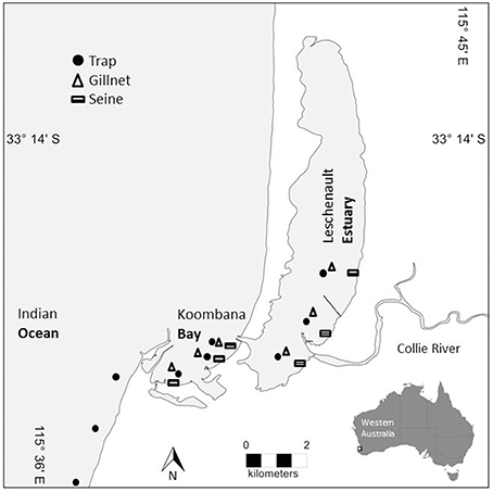
Figure 1. Map of prey sampling sites within the Bunbury study area. Trap sites are denoted with a circle, gillnet sites are denoted with a triangle, and seine net sites are denoted with a rectangle. Sites span the lower reaches of the Leschenault Estuary, the breadth of Koombana Bay (between the Estuary and the coastal water), and the coastal waters (Ocean) outside of the Bay (traps only).

In the marine and estuarine waters near Bunbury, knowledge of potential prey composition and abundance across seasons and habitat regions is critical for understanding the importance of prey as a driving factor in dolphin abundance and distribution patterns. Population trajectories of the local Bunbury fish populations may be negatively influenced by recreational fishing pressure, eutrophication from nutrient enrichment (Potter and Hyndes, 1999), coastal development, vessel activities, and pollution (Hugues-Dit-Ciles et al., 2012). Changes in the fish communities in the shallows of the Leschenault Inlet have been documented since the 1970s using small seine nets (Potter et al., 2000; Veale et al., 2014). The major changes in the Inlet include increases in species associated with warmer water and macroalgae, which correspond to increasing sea temperatures and macroalgal cover. Another recorded change has been a reduction in the density of the longfinned goby Favonigobius lateralis, a species negatively affected by increased siltation (Veale et al., 2014). However, changes in the food quality of dolphin prey, i.e., energy value, have not been investigated. Furthermore, the local fish community has not been sampled with methods other than seine nets since the 1970s and little information is available on the fish communities in the adjacent coastal waters (Potter et al., 2000; Veale et al., 2014).

We hypothesized that dolphin prey availability in different regions of the Bunbury coastal waters would be greater in the summer months when dolphin abundance is highest, and would be greater in the Bay during the summer, as adult female dolphin sightings are more concentrated in the Bay during summer months (Smith et al., 2016). We also hypothesized that energetically rich prey would be present year-round to support the high energetic requirements of pregnant and lactating females that appear to have high affinity to the area.

This study sampled fish and invertebrate prey in three habitat regions (Ocean, Bay, and Estuary) using three types of fishing gear (gillnets, traps, and seine nets) across three summer seasons and two winter seasons between the austral summer of 2008 and austral winter of 2010. Potential dolphin prey were analyzed for energy content to compare the relative quality and quantity of prey between seasons and habitat regions.

Materials and Methods

Study Area

The population of bottlenose dolphins in the Bunbury region, approximately 180 km south of Perth, Western Australia, utilizes the Leschenault Estuary (Estuary), Koombana Bay (Bay), and the near shore coastal waters (Ocean) (Figure 1; Smith et al., 2013; Sprogis et al., 2016a).

The Leschenault Estuary (Estuary) is approximately 13.8 km long, 2.4 km at its widest point and has an average depth of 1.5 m at the trap sites in its lower and middle reaches (Figure 1). The upper estuary has an average depth of less than 1.5 m. The Leschenault Estuary is an example of a reverse salinity gradient system, particularly in the summer months when evaporation leads to hypersaline conditions in the central and northern zones of the estuary (Veale et al., 2014). Many of the fish species that spawn and live in the greater Georgraphe Bay region use the estuary as a nursery area (Potter et al., 2000; Veale et al., 2014). Human impacts on the estuary and near shore areas have been significant over the past century (Hillman et al., 2000; Hugues-Dit-Ciles et al., 2012), including alteration of hydrology, and enrichment from seasonal run-off (Potter et al., 2000; Semeniuk et al., 2000) which has led to excessive algae growth and lowered oxygen levels (Hugues-Dit-Ciles et al., 2012). Increases in urban, agricultural, and industrial land use have led to increases in contaminants into the estuary, which have been further concentrated due to decreases in water input (Hugues-Dit-Ciles et al., 2012).

Koombana Bay (Bay) is approximately 2.3 km long and 2.7 km wide and is located between the Estuary and the coastal waters of Geographe Bay (Figure 1). The hydrology, geomorphology, and flora and fauna of the bay system have been impacted through jetty construction, dredging, breaching of a peninsula to allow boat access between the Bay and the Estuary, sea wall construction, diversion of the Preston River, the construction and deconstruction of a waste water pipeline, and land reclamation and development (Hillman et al., 2000; Semeniuk et al., 2000).

The coastal waters (Ocean) stretch from the southern entrance of Koombana Bay southward (Figure 1). The average depth of the sampling sites along the coast was 10.3 m and the substrate was a mix of sand, rock, and macroalgae. The three sampling sites were approximately 1 km from the low tide mark and spread across a 5 km distance. South-western Australia is a region where tidal fluctuations are generally less than 1 m (i.e., microtidal estuaries Potter and Hyndes, 1999; Tweedley et al., in press) and the lowest annual tide is 0.08 m, while the highest annual tide is 1.16 m. The near shore environment is relatively shallow (<15 m deep).

South-western Australia has a Mediterranean climate with distinct winter wet and summer dry seasons. The long-term, average annual precipitation of Bunbury is 729.1 mm, with the majority of rain falling between June and August (Figure 2) (Bureau of Australian-Bureau-of-Meterology, 2012). The average summer air temperatures range from 13.4 to 29.7°C and from 7 to 18.4°C in winter.

FIGURE 2

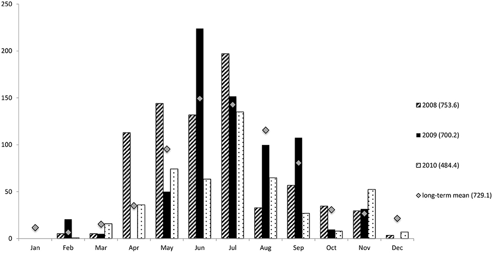
Figure 2. Total rainfall (mm) in Bunbury from 2008–2010. For this study summer constitutes the months of January-March. Winter constitutes the months of June-September to coincide with sampling seasons. Mean monthly data 1995–2012. Numbers in brackets represent the total rainfall of the associated year, or annual mean rainfall 1995–2012. Data courtesy of the Australian Bureau of Meteorology.

Fish Sampling

Three sampling methods (beach seines, gillnets, and Antillean Z-traps, e.g., Sheaves, 1992; Heithaus and Dill, 2002) were used to catch fish and epibenthic invertebrates to provide data on potential dolphin prey availability. These methods sample different habitats and differ in their ability to sample different species effectively, with the seine net used to sample shallow waters, while the gillnet and Z-traps can be used to sample a range of depths. Sampling was carried out in the Austral summer (January to March) and winter months (June to September), between the summer of 2008 and the winter of 2010 (Table 1). No samples were collected in the winter of 2009.

TABLE 1

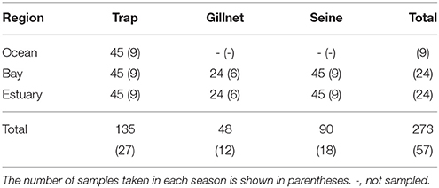
Table 1. The total number of samples taken from each region by trap, gillnet, and seine net during each sampling season (“summer” and “winter”) between January 2008 and September 2010.

The beach seine sampled fish in the shallow waters (<1.5 m deep) close to the shores of the Estuary and Bay, while the gillnets and Z-traps were used to sample in deeper (1–13 m) and more offshore waters. The gillnets were deployed in the Estuary and Bay, whilst the Z-traps were used in all three sampling regions (Figure 1). Within each sampling region, three sites were selected for sampling prey (Figure 1). The sampling sites were spread relatively evenly across the sampling region. In the Estuary, the sampling sites were spread across the navigable waters of the base and lower Estuary, which are described in Veale et al. (2014). No sampling was carried out in the upper Estuary as it is too shallow for vessels to transit. Sites in the Estuary and the southern site in the Bay were in the same location as the long-term sampling sites of the Department of Fisheries Western Australia (see Potter et al., 2000; Gaughan et al., 2006). The sites in the Ocean were spread evenly along the coast at approximately 10–15 m depth.

Three replicates were taken on separate days by both seining and trapping at each site during each season and two replicates were taken by gillnetting at each site (Table 1). Sampling days were spread across the sampling season. The summer season extended from January to mid-March corresponding to the period when dolphins are most abundant in the area, while the winter season extended from June through September when fewer dolphins are present (Smith et al., 2013; Sprogis et al., 2016a).

Beach Seine

The beach seine was 21.5 m long, 1.5 m high, and had 9 mm mesh size in the panels, and 3 mm mesh in the 1.5 m wide codend. The seine was deployed in the Bay and Estuary following the sampling protocol by Ayvazian et al. (2006). One end of the seine was held by a person on the shore as the net was deployed in an arc (semi-circle) by a second person wading through the water before returning to the beach, encircling an area of 73.6 m². The net was then hauled onto the beach, and the catch was immediately placed in buckets of seawater, which were emptied into large plastic bins. Each prey item was identified, counted, measured, and weighed. All surviving fish were subsequently released at the sampling site. Fish that did not survive were bagged, frozen, and taken back to the laboratory for further analysis. The beach seines catch fish in the path of the net and are less effective for fish that are able to avoid the net by going under the lead-line, over the float-line or swimming out of the path of the net (Guest et al., 2003). Seine nets are, however, effective at catching a variety of species and size classes (Dalzell, 1996).

Any dead fish that were not weighed and measured in the field were counted, weighed, and measured in the lab after thawing. When large numbers of a species were caught, a sub-sample of at least 100 individuals was weighed and measured. The total number of individuals was estimated by dividing the total weight of the remaining fish by the mean weight of the sub-sampled fish.

Z-Trap

The Antillean Z-traps were constructed of stainless steel wire mesh and measured approximately 1.1 m long, 0.6 m tall, and 0.6 m wide. The traps were used to sample fish in all three sampling regions and were baited with pilchard (Sardinops saga) in two bait buckets suspended by cable ties within each trap. As catch rates have been shown to decrease with long soak times (e.g., Whitelaw et al., 1991; Sheaves, 1995), the traps were left to soak for 3 h during daylight. After soaking, the traps were retrieved and the catch was transferred to buckets of seawater until they were identified, measured, and counted. All surviving animals were released at the site of capture. It was not possible to accurately weigh fish on the research vessel, and fish were released alive at the sampling site. Therefore, it was not possible to obtain an accurate total biomass of fish captured with the traps. Any fish that did not survive capture were taken back to the laboratory and weighed. Weights were estimated when possible using average length-weight ratios of the same species caught in other regions of this study or by using length-weight curves calculated for the species in other near-shore environments in south-western Australia (Western-Australian-Department-of-Fisheries, unpublished data). The Z-traps sample fish attracted to bait, and under-represents planktivorous fish (Sheaves, 1992). However, fish traps sample a wide range of species and size classes and can be used to sample multiple habitats and locations simultaneously. Fish traps can also be used at depths and in structurally complex habitats inaccessible to net fishing (Sheaves, 1992, 1995). In other studies, Z-traps have captured species not previously captured by net fishing in the same locations, and therefore are useful as a complimentary method to sample a wider range of species (Sheaves, 1992).

Gillnet

A multi-mesh monofilament gillnet was used to capture fish at night in the mid-water column of the Bay and Estuary. Sampling was carried out after sunset to capture diurnal or nocturnally-active species and to limit the visibility of the gillnet to potential dolphin prey. The ocean region was not sampled because of the difficulty in navigating reef areas at night. The net was 120 m long, 1.5 m high and consisted of six 20 m long panels of different mesh size (38, 51, 63, 76, 89, and 102 mm) to maximize the variety and size range of fish captured. Floats were attached along the length of the float line and weights were attached at each end of the lead line to anchor the net in place while it soaked. Reflective tape on the floats and dive flag buoys with flashing lights were used at either end of the net to make it visible after sunset. The gillnet was set perpendicular to the beach just prior to sunset and left for 2–3 h before retrieval. Fish were taken out of the net as it was retrieved and either placed in buckets of seawater or in a seawater ice slurry. Fish that remained alive in the seawater were identified, measured and released at the sampling site. Fish that were placed in the ice slurry were transferred to bags according to mesh size and taken back to the laboratory and frozen for later identification, weighing, measuring, and counting. The research vessel was anchored within 100 m of the net for the duration of the soak period, and the net scanned at 15 min intervals to assess the presence of large schools of fish and to ensure that dolphins did not become entangled in the net. Gillnets can catch a wide variety of species and sizes of fish, depending on the mesh of the net (Dalzell, 1996), and have a comparable catch rate to other passive nets such as trammel nets (Gray et al., 2005).

Captured fish were identified, counted, measured (total length), and wet weighed (g) using a Scout Pro SP 4001 scale.

Environmental and Biotic Measurements

The following physical and environmental variables were recorded at the time of sampling: latitude and longitude, water depth and water temperature, conductivity, pH, and other measurements not used in the analyses presented here. The location was recorded using a geographic positioning system (Garmin GPS72). The water depth was measured using a depth sounder (Raytheon Fish Finder L470) on the research vessel or a graduated measuring stick. The conductivity, temperature, and pH of the water were measured using a TPS Aqua-CP conductivity-TDS-pH-Temperature meter.

Bomb Calorimetry

Prey Samples

The calorific value of 18 different fish species and one crustacean was determined by bomb calorimetry, following the protocol of the bomb calorimeter (Parr, 1969). Fish were selected for bomb calorimetry that either were: (a) very abundant during sampling or (b) were the largest species caught during the first summer and winter sampling seasons. Species that were large in size and most abundant were assumed to be the most likely prey of dolphins (termed potential dolphin prey [PDP]), as they would offer the most efficient exchange between energy exerted while hunting and capturing the prey vs. energy gained through ingestion. Other studies have found that species in the Families Clupeidae, Scombridae, and Sciaenidae are commonly observed items in the stomachs of bottlenose dolphins in other parts of the world (Barros and Odell, 1990; Gannon and Waples, 2004; Spitz et al., 2006; Santos et al., 2007). The energetic values for an additional nine PDP species were estimated using related species from published literature (seven species) and from this study (two species).

Fish were wet weighed and then dried at 60°C until their weights remained constant (typically taking between 24 and 48 h). The dried fish for each species were then ground together in three stages to obtain a fine powder of homogenized fish tissue. The homogenized fish powder was pressed into 1 g pellets and burned in the bomb calorimeter (Parr Instruments 1241 Oxygen bomb calorimeter) with the aid of Parr 45C10 nickel-chromium fuse wire. Water jacket temperatures were recorded prior to firing the oxygen bomb and at one min intervals, until three consecutive readings were stable (typically between 7 and 9 min following the ignition). The heat of combustion was calculated by subtracting the initial temperature reading from the final temperature reading and correcting for the length of fuse wire that burned with the sample pellet. The bomb calorimeter was standardized using benzoic acid powder of a known caloric content (26,433.0 ± 0.0039 KJ/g). A minimum of three replicates of each species were burned.

The calorific content of the tissues was calculated using the following two formulas:

Benzoic acid standardization (Parr, 1969):

$\text{W}=({\text{H}}^{\ast }\text{M}+{\text{e}}_1+{\text{e}}_3)/\text{T},\text{where}:$

W = energy equivalent of the calorimeter (calories/degree Celsius)

H = heat of combustion of the standard benzoic acid sample (calories/gram)

M = mass of the standard benzoic acid sample (grams)

T = net corrected temperature rise (degrees Celsius)

e₁ = correction for heat of formation of nitric acid (calories)

e₃ = correction for heat of combustion of the firing wire (calories)

Gross heat of combustion:

${\text{H}}_{\text{g}}=({\text{T}}^{\ast }\text{W}-{\text{e}}_1-{\text{e}}_2-{\text{e}}_3)/\text{m},\text{where}:$

H_g = gross heat of combustion (calories/gram)

T = t_f- t_a

t_a = temperature at time of firing (Celsius)

t_f = final temperature (Celsius)

e₂ = centimeters of fuse wire consumed in firing

W = energy equivalent of calorimeter (calories/degree Celsius)

m = mass of sample (grams).

The calories per gram of each species was multiplied by the average dry weight for the fish and used to calculate an average calorific value per fish for each species. The average energy value per fish was then multiplied by the total number of fish caught of that species to estimate the total number of calories captured in each region and season by each fishing method.

To estimate the calorific content of other species in this study, energetic values were obtained from the literature and used as a proxy for species caught in the study area. Calories were converted to kilo joules (KJ) for value comparisons with other studies. The average KJ/g wet weight (KJ*g⁻¹) from the proxy species was multiplied by the average weight of the equivalent species from the study to obtain an estimate of the mean KJ per fish.

Analyses of Data

Seasonal and annual means and standard errors were calculated for environmental parameters and the data on total fish biomass and numbers, PDP biomass and numbers, and the number of species.

A nested ANOVA was used to test for differences between seasons and regions, with sites nested within regions (denoted site(region)) for each prey capture method. The main factors in these analyses were region, season, year, site(region), and with the following interaction terms: year*season, season*region, season*site(region), site(region)*year, and year*season*region. The dependent variables tested were the total biomass (log₁₀ transformed), total number of fish (log₁₀ transformed for seine only), and the number of species for each sampling method. Dependent variables were transformed if the Levene's test for normality was significant (Levene, 1960). This type of nested ANOVA design was also used to test for significant differences in the PDP for biomass (log₁₀ transformed), and total number of known KJ of PDP species caught by each method. Analyses were carried out using Statistica 10 (Statsoft, 2014).

Results

Environment

The monthly rainfall during the austral summer months averaged less than 5.3 mm; while in the winter months, it was greater than 107 mm per month (Figure 2). The wettest year of the study was 2008, with a total annual rainfall of 753.6 mm; while the driest year was 2010 (484.4 mm), much drier than in either 2008 or 2009 (700.2 mm), as well as the long-term annual average of 729.1 mm (Figure 2).

The mean salinity did not vary greatly among the three regions in the summers from 2008 to 2010, ranging from about 34 to 35 across these regions (Figure 3A). The mean salinities in the winter of 2008 in the Estuary (32) were lower than in the winter of 2010 (34), which coincided with much higher precipitation in the winter of 2008 than 2010 (418.6 mm compared with 290.2 mm in 2010). Mean salinity varied by only 2.6 across all three regions (Bay = 33–34.5; Estuary = 32.2–34.3; and Ocean = 31.9–34.2).

FIGURE 3

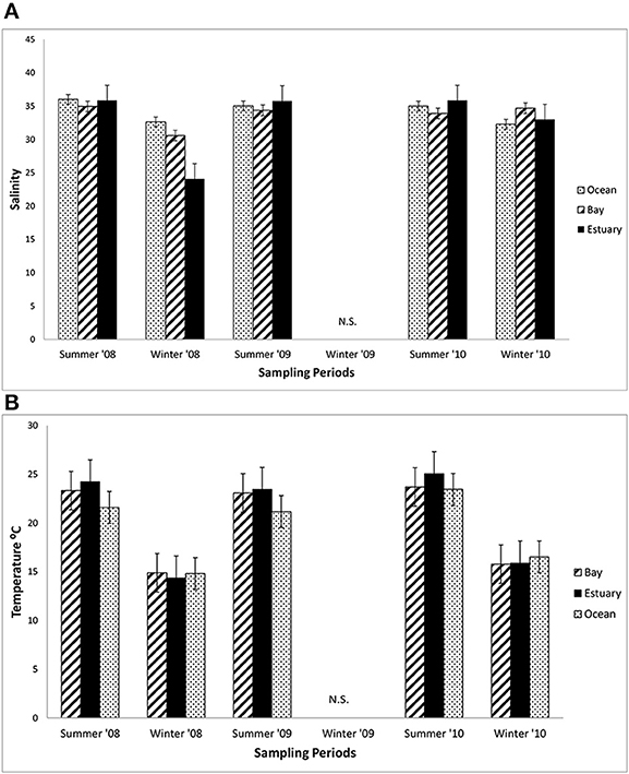
Figure 3. Mean salinity and water temperature. (A) The mean salinity (±1 SE each season) at sampling sites in the Ocean, Bay, and Estuary (N = 9 for Ocean means, N = 24 for Bay and Estuary means). N.S. = Not Sampled. (B) The mean daytime water surface temperature (±1 SE each season) at sampling sites in the Ocean, Bay, and Estuary. (N = 9 for Ocean means, N = 18 for Bay and Estuary means).

Fish Fauna

Overall Abundance and Biomass

A total of 45,729 fish and crustaceans from 35 families, represented by 62 species of teleosts, two species of cephalopod, two species of crustacean, and three species of elasmobranch were captured from all sampling methods during this study (Table 2). More than twice as many fish were captured in summer (mean 12,079.5 ± 159.5) than in winter (7357.5 ± 342.2) (comparing two summer and two winter seasons when all three sampling methods were employed). Greater fish abundance was recorded in the Estuary than the other regions (31,964 in the Estuary, 13,601 in the Bay, and 164 in the Ocean). The most abundant species caught was sandy sprat (Hyperlophus vittatus), contributing 33.6% to the total numbers yet only 1% to the total biomass. Weeping toadfish (Torquigener pleurogramma) made the highest contribution to the total biomass (20%), but constituted only 3.4% of the total numbers. Of the PDP species, blue swimmer crab (Portunas armatus, 17%), trevally (Pseudocaranx sp., 12%), tailor (Pomatomus saltatrix, 10%), and Western Australian salmon (Arripis georgianus, 10%), were the highest contributors to total biomass. A total of 54 species were identified as PDP (Table 2).

TABLE 2

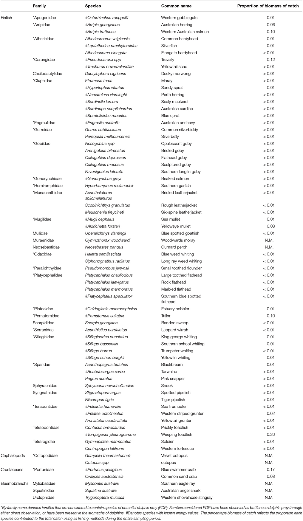
Table 2. The proportional contribution to the total catch by biomass of each species caught by all sampling methods (z-traps, gillnet, and seine) in the Bunbury region between January 2008 and September 2010.

The total biomass of fish caught during this study was 434.14 kg, with 90.39 kg from traps (Table 3), 230.87 kg from gillnets (Table 4), and 85.56 kg from seine (Table 5). Both the overall biomass (291.94 kg) and the PDP biomass (212.94 kg) in the Estuary were twice as heavy as that in the Bay (Total = 131.15 kg; PDP = 119.94 kg). The biomass of PDP species made up 78% of the total biomass caught. The biomass of fish caught in traps from the Ocean was 11.05 kg. Weights were directly obtained or estimated for 59% (n = 17) of the species captured in the traps, which represented 97% (n = 1428) of the fish captured by this method (Table 3).

TABLE 3

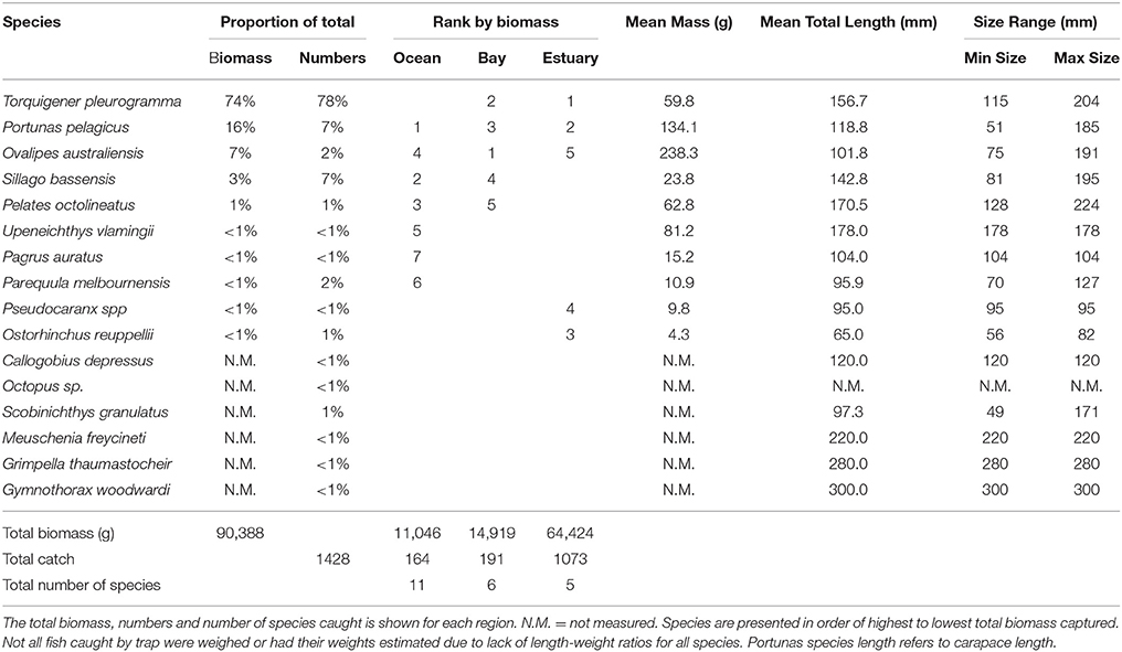
Table 3. Proportion contribution of each species to the total catch in traps by biomass (g) and numbers, and the rank by biomass in the Ocean, Bay, and Estuary.

TABLE 4

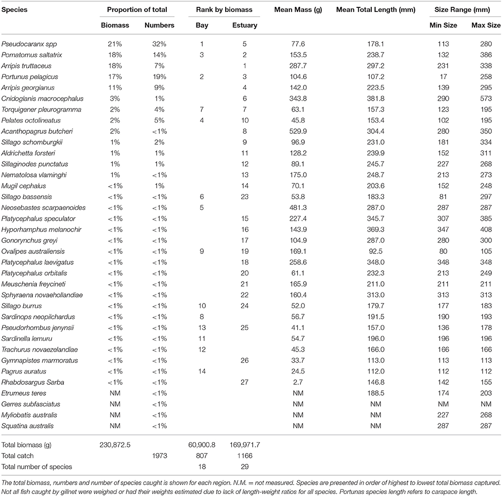
Table 4. Proportion contribution of each species to the total catch in gillnets by biomass (g) and numbers, and the rank by biomass in the Bay, and Estuary.

TABLE 5

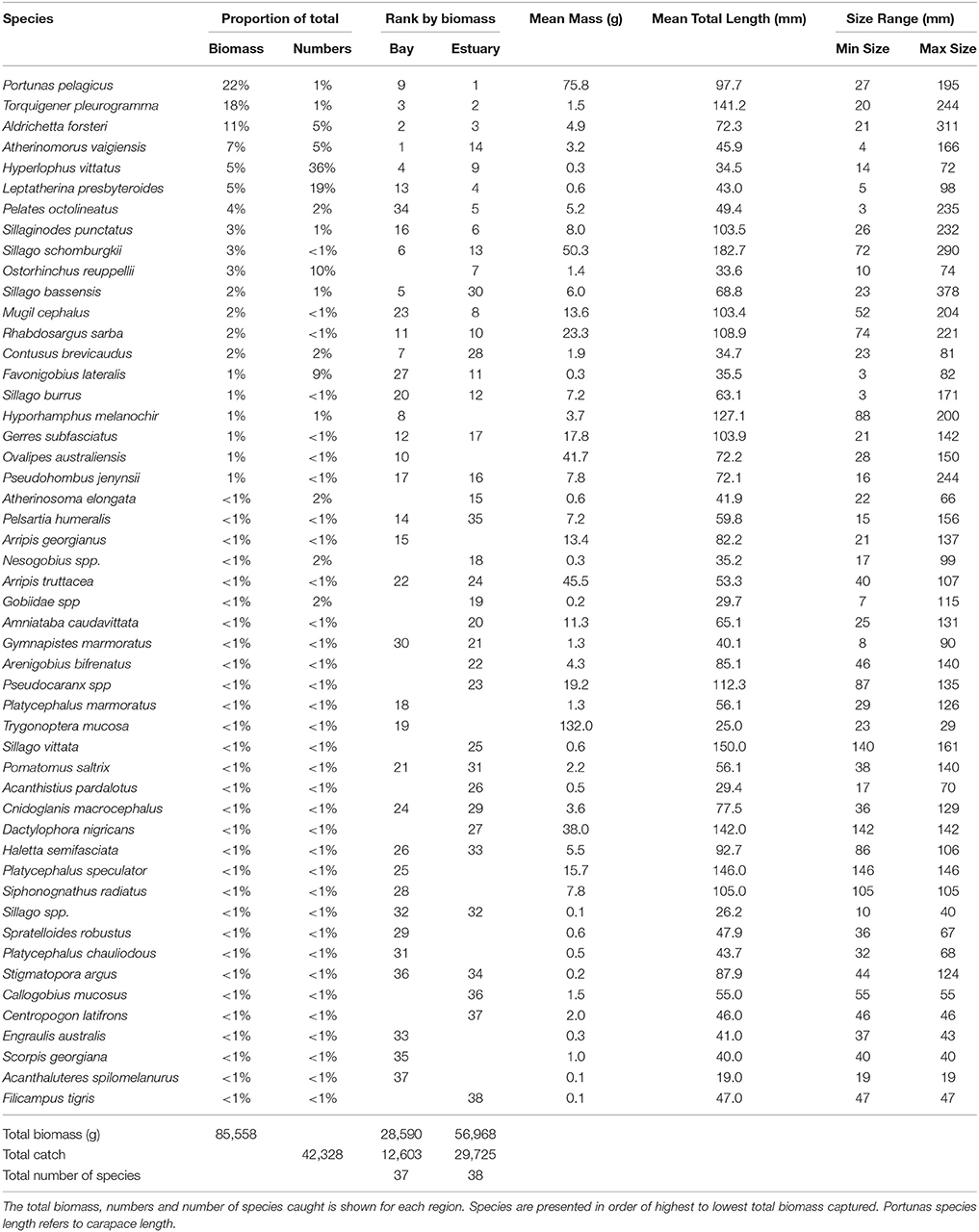
Table 5. Proportion contribution of each species to the total catch in seine nets by biomass (g) and numbers, and the rank by biomass in the Bay, and Estuary.

The toadfish (Tetraodontidae) and crabs (Portunidae) constituted a large portion of the total biomass captured in all seasons and regions of this study (Table 2). Of the PDP, the Portunidae, Pomatomidae (Pomatomus saltatrix), and Arripidae (Arripis georgianus, A. truttaceus) made up the majority of the biomass in the Estuary during the summer. The PDP species caught in the Estuary in winter were dominated by the Arripidae, followed by the Portunidae and Pomatomidae. The biomass of PDP species caught in the Bay during the summer season was more evenly divided among the Pomatomidae, Portunidae, Sillaginidae (Sillago spp.), and others than the distribution of biomasses in the Esturary. The biomass of PDP species caught in the Bay during the winter season was dominated by Carangidae (Pseudocaranx spp), followed by the Portunidae.

Variation in Mean Catches

Z-Traps

The mean total biomass of fish captured in traps was heaviest in the Estuary in all seasons (Figure 4A). The mean biomass caught in the Ocean and Bay were similar, with the exception of winter 2010, when the biomass was heavier in the Bay than the Ocean. The mean biomass of fish in traps differed significantly between seasons (p = 0.02) and among regions (p = 0.04; Table 6A).

FIGURE 4

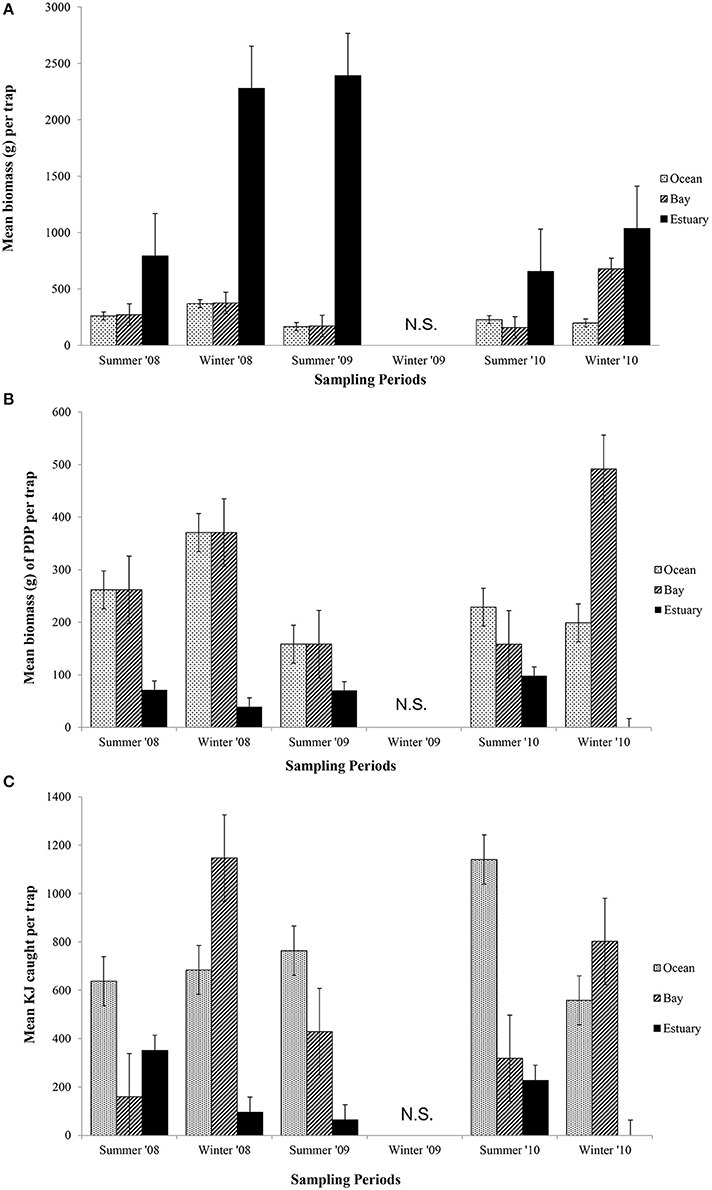
Figure 4. Mean biomass (±1 SE) of prey caught per trap for (A) total biomass; (B) biomass of PDP; and (C) KJ per trap in the Ocean, Bay, and Estuary. N.S. = Not Sampled.

TABLE 6

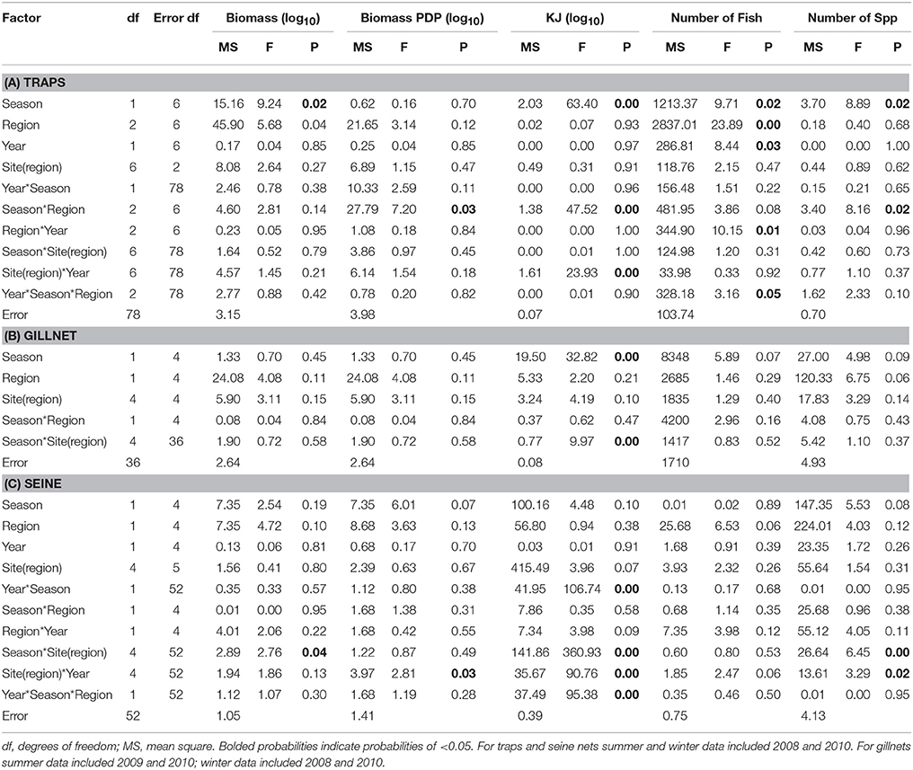
Table 6. Summary of the results of nested ANOVAs to test for seasonal differences in the biomass, PDP biomass, KJ, number of fish, and number of species caught in (A) traps, (B) gillnets, and (C) seine nets between seasons, years and among regions and sites within region.

In contrast to the total biomass, the mean biomass of PDP species in the traps was lighter in the Estuary than in either the Bay or the Ocean (Figure 4B). The mean biomass of PDP species did not differ significantly between the Bay and Ocean, except in winter 2010, when it was markedly heavier in the Bay. The interaction of season and region was the only significant term in the nested ANOVA of PDP biomass (p = 0.04; Table 6A).

The estimated mean total KJ in traps followed a similar pattern among regions and seasons (Figure 4C) to that for the biomass of PDP species (Figure 4B). The season, season*region, and the year*site(region) for the total KJ were all significant (p < 0.0001 for all three terms; Table 6A). When using a nested ANOVA to compare the KJ of the trap catches among years in the summer, the sites within the Estuary showed the most variation. When testing annual differences across summer seasons, the year*site(region) was significant (p < 0.0001; Table 7A).

TABLE 7

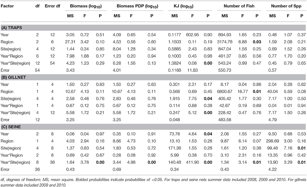
Table 7. Summary of the results of nested ANOVAs to test for annual differences across summer seasons in the biomass, PDP biomass, KJ, number of fish, and number of species caught in (A) traps, (B) gillnets, and (C) seine nets between years and among regions and sites within region.

Gillnet

In general, the mean biomass caught in gillnets was greater in the Estuary than the Bay (Figure 5A), even for species caught in both regions (mean ± 1SE per set for biomass in Estuary = 7082 g ± 1599, Bay = 2538 g ± 1060). However, this difference was not statistically significant, and none of the terms in the nested ANOVA were significant for the total biomass in gillnets (Table 6B). The mean biomass of PDP species showed a virtually identical pattern to that for total biomass (Figure 5B, Table 6B). In contrast to the total biomass and PDP biomass, the KJ caught were not consistently greater in the Estuary than the Bay (Figure 5C) and the KJ caught differed significantly among regions and the season*site(region) was also significant (Table 6B): it was higher in the Bay than the Estuary in the winter of 2008 but was lower in the Bay in the summers of 2009 and 2010 (Figure 5C).

FIGURE 5

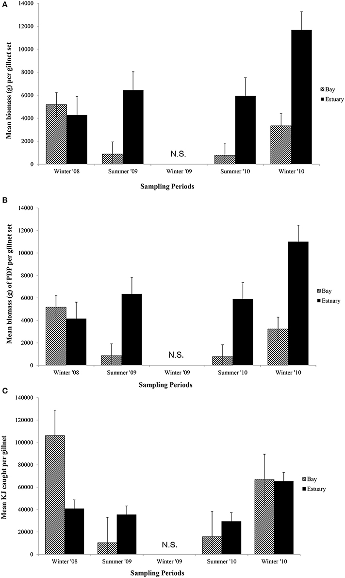
Figure 5. Mean biomass (±1 SE) caught per gillnet set for (A) total biomass; (B) biomass of PDP; and (C) KJ per gillnet in the Bay, and Estuary. N.S. = Not Sampled.

In the seasonal analysis of the gillnet data, significant factors were found only for the number of KJ caught (Table 6B) which differed significantly between seasons (p < 0.0001) and the season*site(region) (p < 0.0001) was significant (Table 6B). The number of KJ caught in the winter seasons were in general higher than those in the summer (Figure 5C). The significant interaction between season and site(region) were attributed to the high variability of gillnet catch from 0 to 253 KJ per set between sites, with the highest variability occurring within the Bay sites during winter.

When comparing the KJ caught in summer seasons among years, the site(region) and season*site(region) was significant (p = 0.04 and p > 0.000, respectively; Table 7B). The number of fish captured by gillnet between summers differed significantly (p = 0.01) between regions (Table 7B). The site(region) term was significant for biomass of PDP (p = 0.05). For the analysis of variation in KJs in winter seasons among years, the year*region (p = 0.04) and year*site(region) (p > 0.000) were significant (Table 8).

TABLE 8

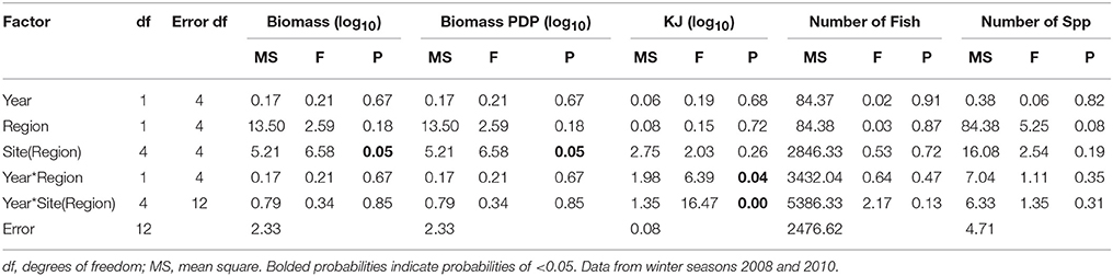
Table 8. Summary of the results of nested ANOVAs to test for annual differences across winter seasons in the biomass, PDP biomass, KJ, number of fish, and number of species caught in gillnets between years and among regions and sites within region.

Beach Seine

The mean biomass per seine set was higher in the Estuary than the Bay during the summer seasons, but in winter was either similar or higher in the Bay than Estuary (Figure 6A). The season*site(region) was significant for the biomass in seines (p = 0.04; Table 6C). This is likely due to the high variability of catch between sites and the much higher biomass caught in the Estuary in the summer of 2008 than in any other season or region (Figure 6A). In the annual analyses, for the three summer seasons, the interaction of year*site(region) was significant (p < 0.0001; Table 7C). The highest summer variability occurred across the Estuary sites (see SE bars on Figure 6A).

FIGURE 6

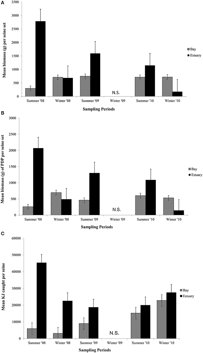
Figure 6. Mean biomass (±1 SE) caught per seine set for (A) total biomass; (B) biomass of PDP; and (C) KJ per seine in the Bay, and Estuary. N.S. = Not Sampled.

Like total biomass, mean biomass of PDP species in seines was highest in the Estuary during the summer seasons, but lower than in the Bay in the winter seasons (Figure 6B). The year*site(region) was significant for seasonal analyses (p = 0.03; Table 6C) and annual analyses (p < 0.0001; Table 7C). Again this is likely due to the high variability of catch among sites, particularly in the summer months, as well as the higher overall biomass caught in 2008 than in 2010. The PDP biomass was less variable in the Estuary than the overall biomass, yet more variable in the middle Bay site due to the significantly higher catch in 2008 than the other summers.

In contrast to PDP biomass, the mean KJ caught per seine was higher in the Estuary in all seasons and years (Figure 6C). The KJ caught was higher in winter than in summer 2010, despite the fact that the biomass of PDP was higher in the summer of that year (Figures 6B,C). The year*season (p < 0.0001), season*site(region) (p < 0.0001), year*site(region) (p < 0.0001), and the year*season*region (p < 0.0001) interactions were all significant for KJ per seine net (Table 6C). Season accounted for the greatest proportion of variation in this analysis due to the large difference in seasonal energy catch in 2008, which was also the year of high variability in the catch between regions. For the annual analyses of KJ per net, year (p = 0.04) and the year*site within region (p < 0.0001) interaction were both significant (Table 7C).

Energy Content

The 19 species selected for bomb calorimetry represented 39% of the seine catches (n = 42.328), 88% of the trap catches (n = 1428), and 97% of the gillnet catches (n = 1973). The energy density of crabs and fish ranged from 2.63 KJ g⁻¹ for Blue swimmer crab (Portunus armatus) to 12.83 KJ g⁻¹ for Western striped grunter (Pelates octolineatus). The average size of each species was used to convert the energy density to a calorific value for whole fish which ranged from 1.81 KJ for Australian anchovy (Engraulis australis) to 2073 KJ for Western Australian salmon (Arripis truttacea) (Table 9). The two species that were captured and analyzed for calorific content in both winter and summer did not show a consistent pattern of variation in calorific content between seasons. The energy value of King George whiting (Sillaginodes punctatus) differed by only 4% between summer and winter, while P. armatus had nearly double the energy content per gram in winter (3.68 KJ g⁻¹) than summer (1.58 KJ g⁻¹). The molt stage of individual P. armatus was not determined and this could have had a significant impact on the energy density of those individuals.

TABLE 9

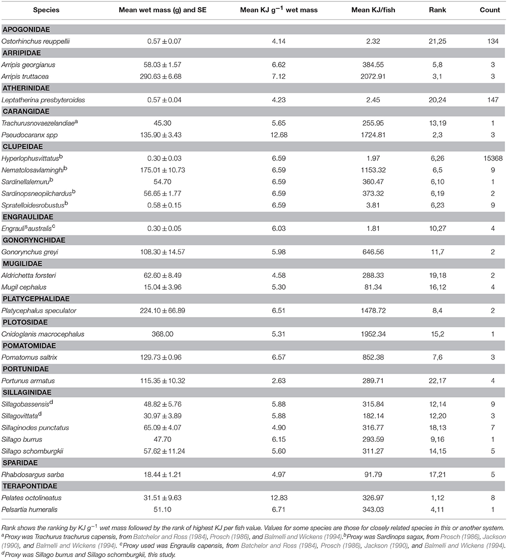
Table 9. Summary of energy values of fish in each family caught in the Estuary, Bay, and Ocean of the Bunbury region.

A higher proportion of the fish with the highest energy density (i.e., >12 KJ g⁻¹) were caught in gillnets in the Bay than in the Estuary in both the summer and winter seasons. While a higher biomass of PDP species were caught in the Estuary than the Bay, higher energy value fish appear to occur in the Bay habitat. A higher proportion of the highest energy density fish were caught in the winter than the summer, which corresponds to the higher biomass in the winter months in the Bay (Figure 5C). The Bay had the highest proportion of the highest energy density fish (84% of the catch), which can be largely attributed to the prevalence of Carangidae species (trevally), which had the 3rd highest KJ/fish of all the fish tested.

The seine catch was dominated by species of low calorific value (<4 KJ g⁻¹), with the exception of the species captured in the Bay during the winter, which had species of both low and medium calorific value (4–6 KJ g⁻¹). The medium value fish were primarily yellow eye mullet (Aldrichetta forsteri). Like the fish captured using the gillnet, higher energy value species were caught in the Bay than the Estuary and winter months had a higher proportion of higher energy fish than the summer months.

Discussion

Understanding predator-prey dynamics is crucial for managing both predator and prey populations. Inferring prey availability from abundance estimates has been the most commonly used method in the marine environment (e.g., Fauchald and Erikstad, 2002; Reilly et al., 2004). However, the nutritional value of prey may be a more critical component of prey value and therefore an important component of any investigation into foraging ecology. In this study, a concomitant increase in abundance of prey was predicted to coincide with the increase in abundance of bottlenose dolphins during summer months off Bunbury, Western Australia (Smith et al., 2013; Sprogis et al., 2016a). The results of prey sampling indicated a higher abundance of prey in the summer seasons, however, the overall biomass and energy density of prey documented were higher in the winters, when fewer dolphins were present, but a time when dolphin mothers and calves remain in the area.

Seasonal and Regional Prey Distribution

The results from sampling potential dolphin prey (PDP) by trap, gillnet, and seine net showed that the patterns of variation in fish abundance, biomass, and energy varied by capture method. As hypothesized, the seine net caught a greater total PDP biomass in the summer than winter seasons. While the numbers of fish caught in seines were higher in the summer, the mean sizes of the most commonly occurring fish were relatively small (<50 mm total length), indicating that dolphins would need to consume high numbers of fish to meet their energetic requirements. Conversely, the trap and gillnet caught more total and PDP biomass in the winter than summer months, which was not expected.

Summer

In the summer months, the number of prey, as well as the total and PDP biomass caught by the seine and gillnet was highest in the Estuary, which does not match the density of adult female dolphin sightings from March 2007 to February 2010, which were highest in the Estuary in the winter (Smith et al., 2016). The mean number of PDP species caught per trap was highest in the Ocean region in the summer months, which was not sampled using the seine or the gillnet.

Winter

In winter months, the gillnet, which sampled larger fish than the seine, caught the highest PDP biomass in the Estuary, which corresponds to the time of higher density of female and calf dolphin sightings in the Estuary (Smith et al., 2016). The seine net had higher catch rates in the Bay in the winter. Likewise, the abundance of PDP species caught by the traps and the gillnet in the Bay was highest in the winter. The density of adult female dolphin sightings were relatively high in both the Bay and Estuary in the winter compared to the summer season, when sightings were concentrated in the Bay (Smith et al., 2016).

Sub-Regions

A comparison between the microhabitats where dolphins forage might be more informative than looking at broad regions alone. A better understanding of microhabitats used for dolphin foraging is important in making informed decisions that impact the microhabitats, such as vessel anchorage, fishing activities, and dredging (Pirotta et al., 2013; Todd et al., 2014). Eierman and Connor (2014) found that bottlenose dolphins in Shark Bay, Australia, foraged preferentially on boundary microhabitats, which were transition areas between seagrass and sand habitats. Barros and Wells (1998) found that bottlenose dolphins along the Gulf coast of Florida foraged predominately over seagrass beds and the majority of their stomach contents consisted of prey species associated with seagrass habitats. In Sarasota Bay, Florida, males foraged predominately on species associated with seagrass beds, while females displayed more individual variation in foraging habits (Rossman et al., 2015a,b). In another study in Sarasota Bay, dolphins selected species associated with mangrove, sandflat, and open bay habitats indicating that there is variability in foraging tactics within a population (McCabe et al., 2010). In the Bunbury region, it has been shown that dolphins rest over sandy substrate and use reef areas for all other behaviors, including foraging (Smith, 2012). Sprogis (2015) found that the benthic association patterns of T. aduncus in this region were sex specific, as seen in Florida. It would be informative to look at the relative availability of seagrass and reef associated prey and compare this to the information on dolphin diets for this population (McCluskey et al., Murdoch University, unpublished data).

Distribution of Predator and Prey

The distribution of dolphins does not match the distribution of prey in the summer months because a higher biomass of PDP and higher proportion of energy-rich prey were caught in the Estuary, rather than the Bay where sightings of adult female dolphins are concentrated in that season (Smith et al., 2016). In summer, dolphins may utilize the Estuary for foraging at night when the water temperature lowers and the risk of predation by sharks decreases. Sharks have been documented to cause injury to dolphins in the study area (Sprogis et al., 2016b). Heithaus and Dill (2002) found that T. aduncus group size and distribution was influenced by the predation risk to tiger sharks (Galeocerdo cuvier) as well as prey availability. Specifically, they found that dolphins in Shark Bay made a trade-off between prey availability and predation risk. Dolphins avoided shallow habitats where prey was more abundant during the warmer months when shark densities were highest, and predation risk was high due to the decreased echolocation efficiency and poor visual detection of sharks due to turbidity and camouflage in the sea grass. Dolphins in the current study utilized the Estuary habitat more in the winter months than in the summer, despite the higher biomass of prey in the summer. This is possibly due to the potential increased predation by sharks in the warmer months, when newborn calves would be at greatest risk. Factors other than prey availability, e.g., reproductive opportunities and predator avoidance, may also be the most influential factors in determining local dolphin abundance in the near-shore waters of our study area. Further studies aimed specifically at understanding the seasonality of shark distribution and abundance are needed to further investigate these factors.

Based on the abundance of prey alone, dolphins would be expected to be sighted more frequently in the Estuary than the Bay, which is not the case for the Bunbury dolphins (Smith et al., 2016). While predators are expected to make choices in their distribution patterns based on the availability (density and location) and quality (energy content) of prey, observations of predator movement and consumption do not always support this theory (Reilly, 1990; Lyons, 1991; van Baalen et al., 2001; Thomas et al., 2011). Reilly (1990) suggested that seasonal dolphin abundance in the Eastern Tropical Pacific was more likely influenced by the ease of capture of prey than prey abundance. Likewise, other studies support the theory that prey patch dynamics, or the catchability of prey, are more important in determining predator distribution than biomass of the prey, particularly for relatively shallow diving cetaceans such as delphinids (Lambert et al., 2014). A more holistic approach to assessing a potential prey field needs to include relative abundance, biomass, energy content, as well as the costs associated with hunting, capturing, and handling each prey species. For example, Thomas et al. (2011) expected harbor seals to take advantage of seasonal pulses of spawning herring, but found that seals consumed more herring in the non-spawning than the spawning season, despite the increased abundance of herring during the spawning months. They concluded that the decreased energy content of the spawning herring, coupled with the fact that juvenile herring required less handling time than adults, influenced the foraging behavior of the harbor seals, rather than the density of the prey alone (Thomas et al., 2011). In the current study, the potential prey was higher quality in the winter than the summer, yet dolphin abundance was lowest in the winter. Smith et al. (2016) found that adult female dolphins in the Bunbury region form stronger associations between individuals in the summer than the winter, which corresponds to when prey is more abundant but of lesser quality. Studies of other social mammals have found that association patterns can be stronger when food is more scarce, as in the case of chaema baboons (Papio hamadryas ursinus) (Henzi et al., 2009); or when food is more abundant, such is the case for killer whales (Orcinus orca) (Foster et al., 2012). Further investigation is therefore necessary to elucidate any relationship between social association and food availability for the Bunbury dolphins.

Seasonal Energy Content and Prey Quality

Since the abundance of dolphins is lower during winters (Smith et al., 2013; Sprogis et al., 2016a), it was hypothesized that prey quantity would be also be lower, but that prey quality would be relatively higher to support the mothers and calves that remain in local waters throughout the winter (Smith et al., 2016), as the energetic cost of lactation and growth is high (Malinowski and Herzing, 2015). As hypothesized, the highest energy contents of fish were generally found in the winter: the highest KJ in traps and gillnets were found in the winter season; while the energy content in the seine net was similar in summer and winter. The overall biomass of PDP and concentration of available energy appears to be higher in the winter seasons, which does not coincide with the higher abundance of dolphins sighted in the summer months.

The suitability of prey includes abundance or biomass, as well as the distribution and ease of capture, all of which influence predator distribution (Benoit-Bird et al., 2013) and population size (Benoit-Bird, 2004). However, assessing the quality (i.e., nutritional value) of available prey may be a better indicator for assessing the value of prey for managing cetacean populations. In a study of the quality of food of Steller sea lions (Eumetopias jubatus), Trites and Donnelly (2003) found that the relative abundance of prey had not changed over time, but the quality of prey had declined, as indicated by a decrease in the abundance of energetically rich species. This led to chronic nutritional stress, a decline in body condition of female Steller sea lions, and subsequent declines in pup production (Pitcher et al., 1998). Other marine mammal populations are likely influenced by the quality of prey available. Endangered resident killer whales (Orcinus orca) in the north-eastern Pacific preferentially forage on Chinook salmon (Oncorhynchus tshawytscha; Ford et al., 1998; Ford and Ellis, 2006), which have the highest energy values of the five species of Pacific salmon, yet occur in the lowest abundance (O'Neill et al., 2014). Common dolphins (Delphinus delphis) also select prey with the highest energy density (>5 KJ g⁻¹) and seem to ignore the most abundant species, which were of lower energy density (<5 KJ g⁻¹) (Spitz et al., 2010a). As the energy value of the prey increased, so did the likelihood of encountering that prey species in the stomachs of the common dolphins, despite the fact that the highest energy fish were encountered in relatively low abundance during trawl surveys (Spitz et al., 2010a). Compared with ten other cetacean species, bottlenose dolphins have medium metabolic requirements and consume medium quality prey (4–6 KJ g⁻¹) (Spitz et al., 2012).

In the current study, the majority of PDP species analyzed for calorific content fell into the category of ‘medium quality prey’ as determined by Spitz et al. (2010b) and the energy content for most species measured were within the range of values recorded from other published values, except for Pseudocaranx spp and Pelates octolineatus, which had very high energy densities (>12 KJ g⁻¹) (Table 9). These values are higher than previously published values of forage fish except for Sardina pilchardus in the Bay of Biscay (4.5–12.1 KJ g⁻¹; Spitz and Jouma'a, 2013). Importantly, Spitz and Jouma'a (2013) found that the species with the highest energy density values were also the species with the highest seasonal and inter-annual variability in energy density. O'Neill et al. (2014) also found that the same species of salmon varied in energy density based on the population sampled. Analyzing the variation of energy density at different temporal and geographic scales for the highest energy fish found in this study would be valuable to ascertain a more accurate picture of energy availability to the dolphins.

Since other studies of prey availability have not recorded the KJ per fish values, it is not possible to compare the proportion of high, medium, and low quality prey captured in the Bunbury region with other systems. The majority of the 19 species analyzed for energy value from this region fell into the medium or high range in terms of energy per fish. The caveat to this is that only fish thought to be PDP were analyzed. While this means that bottlenose dolphins are not as susceptible to decreasing populations of high quality prey as those predator species with the highest energy requirements, bottlenose dolphins would still face nutritional and energetic challenges if only low quality prey were available.

Both the size of the fish and total energy value per fish needs to be considered when evaluating the energy expended by dolphins in foraging and returns on this expenditure. Two of the highest energy fish, Cnidoglanis macrocephalus and Nematolosa vlaminghi had medium KJ g⁻¹ values but high energy content per fish because of their relatively large size. In contrast, P. octolineatus had the highest energy value per gram, yet had a medium to low energy value per fish, indicating that a dolphin would have to expend higher energy capturing more P. octolineatus to take advantage of the energy density of the fish. In total, 35% of the biomass caught was made up of fish representing the highest energy values per fish (i.e., from 647 KJ/fish to 2073 KJ/fish). It is therefore valuable to look at both energy density and absolute energy value per fish when assessing the overall energetic equation of energy gained vs. energy lost from the capture and handling of each prey species.

Furthermore, seasonal variation in energy content may also be important for some species. While only two species (Sillaginodes punctatus and Portunus armatus) were analyzed in this study for seasonal differences, other studies have found marked changes in energy content associated with various environmental and biological factors. Specifically, changes in water temperature and chemical composition, as well as reproductive state and food availability, may influence the lipid and protein composition of prey, thereby shifting the energetic cost-benefit of that particular prey item (Di Beneditto et al., 2009; Spitz and Jouma'a, 2013). In the Baltic Sea, herring (Clupea harengus) have been shown to increase their energy density by up to 250% between seasons (Sveegaard et al., 2012). The energy density of prey can change at the ecosystem level as well as high quality species being removed by human or climatic pressures and replaced by lower quality species (Spitz and Jouma'a, 2013). Increasing the knowledge of calorific value for estuarine and coastal fish species in south-western Australia is therefore important, as well as to understand seasonal changes in energy content of the most important prey species to elucidate the potential value of the prey field.

Prey Sampling using Multiple Catch Methods

Few studies in cetacean foraging ecology have sampled prey availability, and of these, most have used one fishing method only to sample prey (e.g., Heithaus and Dill, 2002; Torres and Read, 2009; McCabe et al., 2010; Kimura et al., 2012; Eierman and Connor, 2014). While each fishing method has its biases and limitations, the aim of using multiple fishing methods in this study was to alleviate some of those limitations. Three types of fishing gear were used in order to sample fish at different depths in different ways (passive, baited, actively sweeping), as well as during daylight and nighttime hours. Each gear had varying levels of catch rate in the different habitat regions. The trends for the mean biomass of all fish and that for PDP caught using the gillnet were similar (97% of the biomass caught by the gillnet was considered to be PDP), unlike the seine net or the traps. The gillnet therefore appears to be a more effective means at targeting species most likely consumed by dolphins in the region. While the traps caught a relatively diverse range of prey in the Ocean region, including cephalopods, the catch in the Bay, and the Estuary, was dominated by the toxic weeping toadfish (Torquigener pleurogramma) and thus was not an efficient means of sampling PDP in this system. Despite the high proportion of small prey caught by the seine net, the catch was still likely to represent the breadth of dolphin prey in the region. Diet studies of dolphins and other marine predators are revealing that smaller prey are often consumed more than expected, likely due to less handling and capture costs of smaller fish, as well as the dense schooling behavior of some small species (Scharf et al., 2000; Thomas et al., 2011). Using three fishing gears proved effective at catching a wider variety of prey than previous studies of the ichthyofauna of the region as this study captured 62 teleost species, compared to the 42 species recorded by Potter et al. (1997; 2000) in the Bay, Estuary, and Collie River using a seine and gillnet. Since four species of fish were captured only in the Ocean, the addition of sampling in the Ocean region does not account for the substantially higher diversity of fish species captured in this study compared to previous studies. Stomach content analyses of the dolphins in the Koombana Bay region will further illuminate the prey preferences of this population (McCluskey et al., Murdoch University, unpublished data).

Conclusion

Ecosystems across the globe have experienced declining biomass and biodiversity in fish stocks (Hilborn et al., 2003; Worm and Myers, 2004; Worm et al., 2006). In many marine systems fisheries have removed or greatly reduced prey species of high energy value, leaving lower quality species to fill the niches left behind by the higher quality species (Ward and Myers, 2005; Myers et al., 2007; Baum and Worm, 2009). This has been documented to cause declines in marine mammal populations, as in the case of steller sea lions (Pitcher et al., 1998; Trites and Donnelly, 2003). Management of predator populations must therefore consider relative prey abundance and availability as well as prey quality, prioritizing the conservation of energetically rich species.

Coastal regions along the coast of south-western Australia, such as those of Bunbury, are experiencing human population growth, port and industrial expansion (Landcorp, 2011), rising recreational fishing pressure, as well as changes to nutrient and chemical input into near-shore marine systems (Hillman et al., 2000; Ayvazian and Nowara, 2001; Hugues-Dit-Ciles et al., 2012). To most effectively manage the apex-predator populations of dolphins in these changing environments, it is important to increase understanding of prey abundance and quality, as well as how human impacts affect those prey communities. This study represents a pioneering investigation into the seasonal and regional prey availability for bottlenose dolphins in an estuarine and coastal environment. It was hypothesized that prey would be more abundant in the summer months, when a higher number of dolphins are present in the local waters. In general, the biomass of prey was greater in the summer than winter months, but the calorific value of prey was higher in the winter. Further, studies are needed to elucidate a more accurate picture of dolphin diet in the study area, such as stomach content analyses, stable isotope, and fatty acid analyses. A better understanding of available prey is critical to managing activities that have direct and indirect effects on those prey species. Specifically, species of medium and high energy density should be prioritized in management decisions related to protecting the bottlenose dolphins in the region. Mating opportunities and predator avoidance are also likely to influence dolphin distribution patterns both seasonally and regionally in the study area and warrant further investigation. This study provides insights into the complex dynamics of predator–prey interactions, and highlights the importance for a better understanding of prey abundance, distribution and calorific content in explaining the spatial ecology of large apex predators.

Ethics Statement

This study was carried under the approval of Murdoch University Animal Ethics Committee (W2114/07) and licensed as scientific research by the Department of Fisheries (2007-20).

Author Contributions

SM, LB, and NL conceived of this study. SM completed all field, laboratory, and data organization work. SM carried out data analyses with assistance from NL. SM led the writing of this manuscript with input from LB and NL. All authors reviewed and approved of the final manuscript.

Funding

We thank our South West Marine Research Program (SWMRP) partners for financial support: Bemax Cable Sands, BHP Billiton Worsley Alumina Ltd., the Bunbury Dolphin Discovery Centre, Bunbury Port Authority, City of Bunbury, Cristal Mining, the Western Australian Department of Parks and Wildlife, Iluka, Millard Marine, Naturaliste Charters, Newmont Boddington Gold, South West Development Commission, and WA Plantation Resources. SM was supported for 3.5 years of her Ph.D. with a Murdoch University International Scholarship.

Conflict of Interest Statement

The authors declare that the research was conducted in the absence of any commercial or financial relationships that could be construed as a potential conflict of interest.

Acknowledgments

We gratefully acknowledge the following people for their assistance with data collection: C. Birdsall, A. Brown, A. Cesario, D. Cori, H. Cross, V. Gillmann, L. Howes, A. Mail, and S. Osterrieder. M. Harvey generously created Figure 1. K. Sprogis provided valuable suggestions on the manuscript.

References

Allen, S. J., Bejder, L., and Krutzen, M. (2011). Why do Indo-Pacific bottlenose dolphins (Tursiops sp.) carry conch shells (Turbinella sp.) in Shark Bay, Western Australia? Mar. Mamm. Sci. 27, 449–454. doi: 10.1111/j.1748-7692.2010.00409.x

CrossRef Full Text | Google Scholar

Australian-Bureau-of-Meterology (2012). Available online at: http://www.bom.gov.au/climate/data/

Ayvazian, S., Craine, M., and Nowara, G. (2006). “Factors affecting the abundance and distribution of recruits (0+) of seven inshore fish species from south-western Australia,” in The Development of a Rigorous Sampling Program for a Long-Term Annual Index of Recruitment for the Finfish Species from South-Western Australia, eds D. Gaughan, S. Ayvazian, G. Nowara, M. Craine and J. Brown (Perth, WA: Department of Fisheries, Western Australia), 43–76.

Ayvazian, S., and Nowara, G. (2001). “West coast estuarine fisheries,” in State of the Fisheries Report 2000-2001, ed. J. Penn (Perth, WA: Department of Fisheries), 22–25.

Balmelli, M., and Wickens, P. A. (1994). Estimates of daily ration for the south-African (Cape) fur-seal. South Afr. J. Marine Sci. Suid Afrikaanse Tydskrif Vir Seewetenskap 14, 151–157. doi: 10.2989/025776194784287111

CrossRef Full Text | Google Scholar

Barros, N. B., and Odell, D. K. (1990). Food habits of bottlenose dolphins in the Southeastern United States. Bottlenose Dolphin 653, 309–328. doi: 10.1016/b978-0-12-440280-5.50020-2

CrossRef Full Text

Barros, N. B., and Wells, R. S. (1998). Prey and feeding patterns of resident bottlenose dolphins (Tursiops truncatus) in Sarasota Bay, Florida. J. Mammal. 79, 1045–1059. doi: 10.2307/1383114

CrossRef Full Text | Google Scholar

Batchelor, A. L., and Ross, G. J. B. (1984). The diet and implications of dietary change of Cape gannets on Bird Island, Algoa Bay. Ostrich 55, 45–63. doi: 10.1080/00306525.1984.9634757

CrossRef Full Text | Google Scholar

Baum, J. K., and Worm, B. (2009). Cascading top-down effects of changing oceanic predator abundances. J. Ani. Ecol. 78, 699–714. doi: 10.1111/j.1365-2656.2009.01531.x

PubMed Abstract | CrossRef Full Text | Google Scholar

Bax, N. J. (1998). The significance and prediction of predation in marine fisheries. ICES J. Mar. Sci. 55, 997–1030. doi: 10.1006/jmsc.1998.0350

CrossRef Full Text | Google Scholar

Benoit-Bird, K. J. (2004). Prey caloric value and predator energy needs: foraging predictions for wild spinner dolphins. Mar. Biol. 145, 435–444. doi: 10.1007/s00227-004-1339-1

CrossRef Full Text | Google Scholar

Benoit-Bird, K. J., Battaile, B. C., Heppell, S. A., Hoover, B., Irons, D., Jones, N., et al. (2013). Prey patch patterns predict habitat use by top marine predators with diverse foraging strategies. PLoS ONE 8:e53348. doi: 10.1371/journal.pone.0053348

PubMed Abstract | CrossRef Full Text | Google Scholar

Dalzell, P. (1996). “Catch rates, selectivity and yields of reef fishing,” in Reef Fisheries, eds N. V. C. Polunin and C. M. Roberts (London: Springer), 161–192.

Google Scholar

Di Beneditto, A. P. M., Dos Santos, M. V. B., and Vidal, M. V. (2009). Comparison between the diet of two dolphins from south-eastern Brazil: proximate-composition and caloric value of prey species. J. Mar. Biol. Assoc. U.K. 89, 903–905. doi: 10.1017/S0025315409001519

CrossRef Full Text | Google Scholar

Eierman, L. E., and Connor, R. C. (2014). Foraging behavior, prey distribution, and microhabitat use by bottlenose dolphins Tursiops truncatus in a tropical atoll. Mar. Ecol. Prog. Ser. 503, 279–288. doi: 10.3354/meps10721

CrossRef Full Text | Google Scholar

Fauchald, P., and Erikstad, K. E. (2002). Scale-dependent predator-prey interactions: the aggregative response of seabirds to prey under variable prey abundance and patchiness. Mar. Ecol. Prog. Ser. 231, 279–291. doi: 10.3354/meps231279

CrossRef Full Text | Google Scholar

Ford, J. K. B., and Ellis, G. M. (2006). Selective foraging by fish-eating killer whales Orcinus orca in British Columbia. Mar. Ecol. Progr. Ser. 316, 185–199. doi: 10.3354/meps316185

CrossRef Full Text | Google Scholar

Ford, J. K. B., Ellis, G. M., Barrett-Lennard, L. G., Morton, A. B., Palm, R. S., and Iii, K. C. B. (1998). Dietary specialization in two sympatric populations of killer whales (Orcinus orca) in Coastal British Columbia and Adjacent Waters. Can. J. Zool. 76, 1456–1471. doi: 10.1139/cjz-76-8-1456

CrossRef Full Text | Google Scholar

Foster, E. A., Franks, D. W., Morrell, L. J., Balcomb, K. C., Parsons, K. M., Van Ginneken, A., et al. (2012). Social network correlates of food availability in an endangered population of killer whales, Orcinus orca. Anim. Behav. 83, 731–736. doi: 10.1016/j.anbehav.2011.12.021

CrossRef Full Text | Google Scholar

Gannon, D. P., and Waples, D. M. (2004). Diets of coastal bottlenose dolphins from the US mid-Atlantic coast differ by habitat. Mar. Mamm. Sci. 20, 527–545. doi: 10.1111/j.1748-7692.2004.tb01177.x

CrossRef Full Text | Google Scholar

Gaughan, D., Ayvazian, S., Nowara, G., Craine, M., and Brown, J. (2006). “The development of a rigorous sampling program for the long-term index of recruitment for finfish species from south-western Western Australia,” in Final FRDC Report– Project 1999/153 (Perth, WA: Department of Fisheries).

Gray, C. A., Jones, M. V., Rotherham, D., Broadhurst, M. K., Johnson, D. D., and Barnes, L. M. (2005). Utility and efficiency of multi-mesh gill nets and trammel nets for sampling assemblages and populations of estuarine fish. Mar. Freshw. Res. 56, 1077–1088. doi: 10.1071/MF05056

CrossRef Full Text | Google Scholar

Guest, M. A., Connolly, R. M., and Loneragan, N. R. (2003). Seine nets and beam trawls compared by day and night for sampling fish and crustaceans in shallow seagrass habitat. Fish. Res. 64, 185–196. doi: 10.1016/S0165-7836(03)00109-7

CrossRef Full Text | Google Scholar

Heithaus, M. R., and Dill, L. M. (2002). Food availability and tiger shark predation risk influence bottlenose dolphin habitat use. Ecology 83, 480–491. doi: 10.1890/0012-9658(2002)083[0480:FAATSP]2.0.CO;2

CrossRef Full Text | Google Scholar

Heithaus, M. R., and Dill, L. M. (2006). Does tiger shark predation risk influence foraging habitat use by bottlenose dolphins at multiple spatial scales? OIKOS 114, 257–264. doi: 10.1111/j.2006.0030-1299.14443.x

CrossRef Full Text | Google Scholar

Heithaus, M. R., Frid, A., Wirsing, A. J., and Worm, B. (2008). Predicting ecological consequences of marine top predator declines. Trends Ecol. Evol. 23, 202–210. doi: 10.1016/j.tree.2008.01.003

PubMed Abstract | CrossRef Full Text | Google Scholar

Henzi, S., Lusseau, D., Weingrill, T., Van Schaik, C., and Barrett, L. (2009). Cyclicity in the structure of female baboon social networks. Behav. Ecol. Sociobiol. 63, 1015–1021. doi: 10.1007/s00265-009-0720-y

CrossRef Full Text | Google Scholar

Hernandez-Milian, G., Begoña Santos, M., Reid, D., and Rogan, E. (2015). Insights into the diet of Atlantic white-sided dolphins (Lagenorhynchus acutus) in the Northeast Atlantic. Mar. Mammal Sci. doi: 10.1111/mms.12272. [Epub ahead of print].

CrossRef Full Text | Google Scholar

Hilborn, R., Branch, T. A., Ernst, B., Magnusson, A., Minte-Vera, C. V., Scheuerell, M. D., et al. (2003). State of the world's fisheries. Annu. Rev. Environ. Resour. 28, 359–399. doi: 10.1146/annurev.energy.28.050302.105509

CrossRef Full Text | Google Scholar

Hillman, K., Mccomb, A., Bastyan, G., and Paling, E. (2000). Macrophyte abundance and distribution in Leschenault Inlet, an estuarine system in south-western Australia. J. R. Soc. West. Aust. 83, 349–355.

Google Scholar

Hugues-Dit-Ciles, J., Kelsey, P., Marillier, B., Robb, M., Forbes, V., and McKenna, M. (2012). Leschenault Estuary Water Quality Improvement Plan. Perth, WA: Department of Water.

Jackson, S. (1990). Seabird Digestive Physiology in Relation to Foraging Ecology. PhD. University of Cape Town.

Kimura, S., Akamatsu, T., Li, S., Dong, L., Wang, K., Wang, D., et al. (2012). Seasonal changes in the local distribution of Yangtze finless porpoises related to fish presence. Mar. Mamm. Sci. 28, 308–324. doi: 10.1111/j.1748-7692.2011.00490.x

CrossRef Full Text | Google Scholar

Lambert, C., Mannocci, L., Lehodey, P., and Ridoux, V. (2014). Predicting cetacean habitats from their energetic needs and the distribution of their prey in two contrasted tropical regions. PLoS ONE 9:e105958. doi: 10.1371/journal.pone.0105958

PubMed Abstract | CrossRef Full Text | Google Scholar

Landcorp (2011). Available online at: http://www.landcorp.com.au/project/bunburywaterfront [Online]. [Accessed 2014].

Levene, H. (1960). Robust tests for equality of variances. Contrib. Probab. Statist. Essays Honor Harold Hotel. 2, 278–292.

Lyons, K. J. (1991). Variation in Feeding Behavior of Female Sea Otters, Enhydra lutris, Between Individuals and with Reproductive Condition. Santa Cruz, CA: University of California.

Malinowski, C. R., and Herzing, D. L. (2015). Prey use and nutritional differences between reproductive states and age classes in Atlantic spotted dolphins (Stenella frontalis) in the Bahamas. Mar. Mamm. Sci. 31, 1471–1493. doi: 10.1111/mms.12238

CrossRef Full Text | Google Scholar

McCabe, E. J. B., Gannon, D. P., Barros, N. B., and Wells, R. S. (2010). Prey selection by resident common bottlenose dolphins (tursiops truncatus) in Sarasota Bay, Florida. Mar. Biol. 157, 931–942. doi: 10.1007/s00227-009-1371-2

CrossRef Full Text | Google Scholar

McCluskey, S. M., and Lewison, R. L. (2008). Quantifying fishing effort: a synthesis of current methods and their applications. Fish Fisher. 9, 188–200. doi: 10.1111/j.1467-2979.2008.00283.x

CrossRef Full Text | Google Scholar

Meynier, L., Pusineri, C., Spitz, J., Santos, M. B., Pierce, G. J., and Ridoux, V. (2008). Intraspecific dietary variation in the short-beaked common dolphin Delphinus delphis in the Bay of Biscay: importance of fat fish. Mar. Ecol. Progr. Ser. 354, 277–287. doi: 10.3354/meps07246

CrossRef Full Text | Google Scholar

Myers, R. A., Baum, J. K., Shepherd, T. D., Powers, S. P., and Peterson, C. H. (2007). Cascading effects of the loss of apex predatory sharks from a coastal ocean. Science 315, 1846–1850. doi: 10.1126/science.1138657

PubMed Abstract | CrossRef Full Text | Google Scholar

O'Donoghue, M., Boutin, S., Krebs, C. J., Murray, D. L., and Hofer, E. J. (1998). Behavioural responses of coyotes and lynx to the snowshoe hare cycle. OIKOS 82, 169–183. doi: 10.2307/3546927

CrossRef Full Text | Google Scholar

O'Neill, S. M., Ylitalo, G. M., and West, J. E. (2014). Energy content of Pacific Salmon as prey of northern and southern resident killer whales. Endangered Species Res. 25, 265–281. doi: 10.3354/esr00631

CrossRef Full Text | Google Scholar

Parr (1969). Operating Instructions for the 1241 Oxygen Bomb Calorimeter [Online]. Available online at: http://wweb.uta.edu/faculty/timmons/bomb-calorimeter-manual.pdf [Accessed 2008].

Pirotta, E., Laesser, B. E., Hardaker, A., Riddoch, N., Marcoux, M., and Lusseau, D. (2013). Dredging displaces bottlenose dolphins from an urbanised foraging patch. Mar. Pollut. Bull. 74, 396–402. doi: 10.1016/j.marpolbul.2013.06.020

PubMed Abstract | CrossRef Full Text | Google Scholar

Pitcher, K. W., Calkins, D. G., and Pendleton, G. W. (1998). Reproductive performance of female steller sea lions: an energetics-based reproductive strategy? Can. J. Zool. Rev. Can. De Zool. 76, 2075–2083. doi: 10.1139/z98-149

CrossRef Full Text | Google Scholar

Potter, I. C., Chalmer, P. N., Tiivel, D. J., Steckis, R. A., Platell, M. E., and Lenanton, R. C. J. (2000). The fish fauna and finfish fishery of the Leschenault Estuary in south-western Australia. J. R. Soc. West. Aust. 83, 481–501.

Google Scholar

Potter, I. C., and Hyndes, G. A. (1999). Characteristics of the ichthyofaunas of southwestern Australian estuaries, including comparisons with holarctic estuaries and estuaries elsewhere in temperate Australia: a review. Aust. J. Ecol. 24, 395–421. doi: 10.1046/j.1442-9993.1999.00980.x

CrossRef Full Text | Google Scholar

Potter, I. C., Tiivel, D. J., Valesini, F. J., and Hyndes, G. A. (1997). Comparisons between the ichthyofaunas of a temperate lagoonal-like estuary and the embayment into which that estuary discharges. Int. J. Salt Lake Res. 5, 337–358. doi: 10.1007/BF01995386

CrossRef Full Text | Google Scholar

Prosch, R. M. (1986). The Biology, Distribution and Ecology of Lampanyctodes hectoris and Maurolicus Muelleri Along the South-African Coast. M.Sc., University of Cape Town.

Reilly, S. B. (1990). Seasonal-changes in the distribution and habitat differences among dolphins in the eastern tropical Pacific. Mar. Ecol. Progr. Ser. 66, 1–11. doi: 10.3354/meps066001

CrossRef Full Text | Google Scholar

Reilly, S., Hedley, S., Borberg, J., Hewitt, R., Thiele, D., Watkins, J., et al. (2004). Biomass and energy transfer to baleen whales in the South Atlantic sector of the Southern Ocean. Deep Sea Res. II Top. Stud. Oceanogr. 51, 1397–1409. doi: 10.1016/S0967-0645(04)00087-6

CrossRef Full Text | Google Scholar

Rossman, S., Berens McCabe, E., Barros, N. B., Gandhi, H., Ostrom, P. H., Stricker, C. A., et al. (2015a). Foraging habits in a generalist predator: sex and age influence habitat selection and resource use among bottlenose dolphins (Tursiops truncatus). Mar. Mamm. Sci. 31, 155–168. doi: 10.1111/mms.12143

CrossRef Full Text | Google Scholar

Rossman, S., Ostrom, P. H., Stolen, M., Barros, N. B., Gandhi, H., Stricker, C. A., et al. (2015b). Individual specialization in the foraging habits of female bottlenose dolphins living in a trophically diverse and habitat rich estuary. Oecologia 178, 415–425. doi: 10.1007/s00442-015-3241-6

PubMed Abstract | CrossRef Full Text | Google Scholar

Santos, M. B., Fernandez, R., Lopez, A., Martinez, J. A., and Pierce, G. J. (2007). Variability in the diet of bottlenose dolphin, Tursiops truncatus in Galician waters, north-western Spain, 1990-2005. J. Mar. Biol. Assoc. U.K. 87, 231–241. doi: 10.1017/S0025315407055233

CrossRef Full Text | Google Scholar

Sargeant, B. L., Mann, J., Berggren, P., and Krutzen, M. (2005). Specialization and development of beach hunting, a rare foraging behavior, by wild bottlenose dolphins (Tursiops sp.). Can. J. Zool. Rev. Can. De Zool. 83, 1400–1410. doi: 10.1139/z05-136

CrossRef Full Text | Google Scholar

Scharf, F. S., Juanes, F., and Rountree, R. A. (2000). Predator size-prey size relationships of marine fish predators: interspecific variation and effects of ontogeny and body size on trophic-niche breadth. Mar. Ecol. Prog. Ser. 208, 229–248. doi: 10.3354/meps208229

CrossRef Full Text | Google Scholar

Semeniuk, V., Semeniuk, T. A., and Unno, J. (2000). The Leschenault Inlet estuary: an overview. J. R. Soc. West. Aust. 83, 207–228.

Google Scholar

Sheaves, M. J. (1992). Patterns of distribution and abundance of fishes in different habitats of a mangrove-lined tropical estuary, as determined by fish trapping. Aust. J. Mar. Freshw. Res. 43, 1461–1479. doi: 10.1071/MF9921461

CrossRef Full Text | Google Scholar

Sheaves, M. J. (1995). Effect of design modifications and soak time variations on Antillean-Z Fish trap performance in a tropical estuary. Bull. Mar. Sci. 56, 475–489.

Google Scholar

Smith, H. C. (2012). Population Dynamics and Habitat Use of Bottlenose Dolphins (Tursiops Aduncus). PhD. Murdoch University, Bunbury, WA.

Smith, H. C., Frere, C., Kobryn, H. T., and Bejder, L. (2016). Seasonal cyclicity of associations, habitat use and calving by adult female bottlenose dolphins: informing management. Anim. Conserv. 19. doi: 10.1111/acv.12263

CrossRef Full Text

Smith, H. C., Pollock, K., Waples, K., Bradley, S., and Bejder, L. (2013). Use of the robust design to estimate seasonal abundance and demographic parameters of a coastal bottlenose dolphin (Tursiops aduncus) population. PLoS ONE 8:e76574. doi: 10.1371/annotation/369119db-d9ca-4473-9390-89ee0c2a532f

PubMed Abstract | CrossRef Full Text | Google Scholar

Spitz, J., and Jouma'a, J. (2013). Variability in energy density of forage fishes from the Bay of Biscay (north-east Atlantic Ocean): reliability of functional grouping based on prey quality. J. Fish Biol. 82, 2147–2152. doi: 10.1111/jfb.12142

PubMed Abstract | CrossRef Full Text | Google Scholar

Spitz, J., Mourocq, E., Leaute, J. P., Quero, J. C., and Ridoux, V. (2010a). Prey selection by the common dolphin: fulfilling high energy requirements with high quality food. J. Exp. Mar. Biol. Ecol. 390, 73–77. doi: 10.1016/j.jembe.2010.05.010

CrossRef Full Text | Google Scholar

Spitz, J., Mourocq, E., Schoen, V., and Ridoux, V. (2010b). Proximate composition and energy content of forage species from the Bay of Biscay: high- or low-quality food? ICES J. Mar. Sci. 67, 909–915. doi: 10.1093/icesjms/fsq008

PubMed Abstract | CrossRef Full Text | Google Scholar

Spitz, J., Rousseau, Y., and Ridoux, V. (2006). Diet overlap between harbour porpoise and bottlenose dolphin: an argument in favour of interference competition for food? Estuar. Coast. Shelf Sci. 70, 259–270. doi: 10.1016/j.ecss.2006.04.020

CrossRef Full Text | Google Scholar

Spitz, J., Trites, A. W., Becquet, V., Brind'amour, A., Cherel, Y., Galois, R., et al. (2012). Cost of living dictates what whales, dolphins and porpoises eat: the importance of prey quality on predator foraging strategies. PLoS ONE 7:e50096. doi: 10.1371/journal.pone.0050096

PubMed Abstract | CrossRef Full Text | Google Scholar

Sprogis, K. R. (2015). Sex-Specific Patterns in Abundance, Home Ranges and Habitat Use of Indo-Pacific Bottlenose Dolphins (Tursiops aduncus) in South-Western Australia. Ph.D. thesis, Murdoch University, Perth.

Sprogis, K. R., Pollock, K. H., Raudino, H. C., Allen, S. J., Kopps, A. M., Manlik, O., et al. (2016a). Sex-specific patterns in abundance, temporary emigration and survival of Indo-Pacific bottlenose dolphins (Tursiops aduncus) in coastal and estuarine waters. Front. Mar. Sci. 3:12. doi: 10.3389/fmars.2016.00012

CrossRef Full Text | Google Scholar

Sprogis, K. R., Raudino, H. C., Rankin, R., MacLeod, C. D., and Bejder, L. (2016b). Home range size of adult Indo-Pacific bottlenose dolphins (Tursiops aduncus) in a coastal and estuarine system is habitat and sex-specific. Mar. Mamm. Sci. 32, 287–308. doi: 10.1111/mms.12260

CrossRef Full Text | Google Scholar

Statsoft (2014). Statistica, advanced edition [Online]. Tulsa, OK.

Sveegaard, S., Andreasen, H., Mouritsen, K. N., Jeppesen, J. P., Teilmann, J., and Kinze, C. C. (2012). Correlation between the seasonal distribution of harbour porpoises and their prey in the Sound, Baltic Sea. Mar. Biol. 159, 1029–1037. doi: 10.1007/s00227-012-1883-z

CrossRef Full Text | Google Scholar

Thomas, A. C., Lance, M. M., Jeffries, S. J., Miner, B. G., and Acevedo-Gutierrez, A. (2011). Harbor seal foraging response to a seasonal resource pulse, spawning Pacific herring. Mar. Ecol. Progr. Ser. 441, 225–239. doi: 10.3354/meps09370

CrossRef Full Text | Google Scholar

Todd, V. L. G., Todd, I. B., Gardiner, J. C., Morrin, E. C. N., Macpherson, N. A., Dimarzio, N. A., et al. (2014). A review of impacts of marine dredging activities on marine mammals. ICES J. Mar. Sci. 72, 328–340. doi: 10.1093/icesjms/fsu187

CrossRef Full Text | Google Scholar

Torres, L. G., and Read, A. J. (2009). Where to catch a fish? The influence of foraging tactics on the ecology of bottlenose dolphins (Tursiops truncatus) in Florida Bay, Florida. Mar. Mamm. Sci. 25, 797–815. doi: 10.1111/j.1748-7692.2009.00297.x

CrossRef Full Text | Google Scholar

Torres, L. G., Read, A. J., and Halpin, P. (2008). Fine-scale habitat modeling of a top marine predator: do prey data improve predictive capacity? Ecol. Appl. 18, 1702–1717. doi: 10.1890/07-1455.1

PubMed Abstract | CrossRef Full Text | Google Scholar

Trites, A. W., and Donnelly, C. P. (2003). The decline of steller sea lions Eumetopias jubatus in Alaska: a review of the nutritional stress hypothesis. Mamm. Rev. 33, 3–28. doi: 10.1046/j.1365-2907.2003.00009.x

CrossRef Full Text | Google Scholar

Tweedley, J. R., Warwick, R. M., and Potter, I. C. (in press). The contrasting ecology of macrotidal microtidal estuaries. Oceanogr. Mar. Biol. Annu. Rev.

van Baalen, M., Krivan, V., Rijn, P. C. J. V., and Sabelis, M. W. (2001). Alternative food, switching predators, and the persistence of predator-prey systems. Am. Nat. 157, 512–524. doi: 10.1086/319933

PubMed Abstract | CrossRef Full Text | Google Scholar

Veale, L., Tweedley, J. R., Clarke, K. R., Hallett, C. S., and Potter, I. C. (2014). Characteristics of the ichthyofauna of a temperate microtidal estuary with a reverse salinity gradient, including inter-decadal comparisons. J. Fish Biol. 85, 1320–1354. doi: 10.1111/jfb.12467

PubMed Abstract | CrossRef Full Text | Google Scholar

Ward, P., and Myers, R. A. (2005). Shifts in open-ocean fish communities coinciding with the commencement of commercial fishing. Ecology 86, 835–847. doi: 10.1890/03-0746

CrossRef Full Text | Google Scholar

Whitelaw, A. W., Sainsbury, K. J., Dews, G. J., and Campbell, R. A. (1991). Catching characteristics of 4 fish-trap types on the north-west shelf of Australia. Aust. J. Mar. Freshwater Res. 42, 369–382. doi: 10.1071/MF9910369

CrossRef Full Text | Google Scholar

Wirsing, A. J., Heithaus, M. R., and Dill, L. M. (2007). Can measures of prey availability improve our ability to predict the abundance of large marine predators? Oecologia 153, 563–568. doi: 10.1007/s00442-007-0769-0

PubMed Abstract | CrossRef Full Text | Google Scholar

Wirsing, A. J., Heithaus, M. R., Frid, A., and Dill, L. M. (2008). Seascapes of fear: evaluating sublethal predator effects experienced and generated by marine mammals. Mar. Mamm. Sci. 24, 1–15. doi: 10.1111/j.1748-7692.2007.00167.x

CrossRef Full Text | Google Scholar

Worm, B., Barbier, E. B., Beaumont, N., Duffy, J. E., Folke, C., Halpern, B. S., et al. (2006). Impacts of biodiversity loss on ocean ecosystem services. Science 314, 787–790. doi: 10.1126/science.1132294

PubMed Abstract | CrossRef Full Text | Google Scholar

Worm, B., and Branch, T. A. (2012). The future of fish. Trends Ecol. Evol. 27, 594–599. doi: 10.1016/j.tree.2012.07.005

PubMed Abstract | CrossRef Full Text | Google Scholar

Worm, B., Hilborn, R., Baum, J. K., Branch, T. A., Collie, J. S., Costello, C., et al. (2009). Rebuilding global fisheries. Science 325, 578–585. doi: 10.1126/science.1173146

PubMed Abstract | CrossRef Full Text | Google Scholar

Worm, B., and Myers, R. A. (2004). Managing fisheries in a changing climate - No need to wait for more information: industrialized fishing is already wiping out stocks. Nature 429, 15–15. doi: 10.1038/429015a

CrossRef Full Text | Google Scholar