Recent Arctic Sea Level Variations from Satellites

Introduction

For the Arctic region, a reasonable number of tide gauge data is available along the Norwegian and Russian coasts since 1950, and most of published research on Arctic sea level extends cautiously from these areas (i.e., Pavlov, 2001; Proshutinsky et al., 2004; Henry et al., 2012). However, only a limited amount of data is available in the interior of the Arctic Ocean, and records with a length of several decades, are completely absent outside the Norwegian and Russian sectors.

Since the early 1990s, ERS-1, ERS-2, and ENVISAT satellites have been able to map the Arctic Ocean sea level up to the 82° parallel whenever the Ocean is not frozen. In 2010 CryoSat-2 satellite was launched, ensuring continuity to altimetric records until present, and extending the spatial coverage up to 88°N significantly improving our ability to retrieve sea level in ocean leads (Stenseng and Andersen, 2012).

Basin scale changes in sea level are primarily caused by two processes: variation in temperature and salinity and through the exchange of water masses between different basins and/or land reservoirs (Leuliette, 2014). The Arctic Ocean is classified as a Mediterranean sea because of its limited water exchange with other ocean basins and because its circulation is coupled with thermohaline differences (Tomczak and Godfrey, 2003). Internally in the Arctic Large Ocean mass variations can be found mainly driven by wind forcing (Volkov and Landerer, 2013; Volkov, 2014).

In this paper we present an updated version of the DTU Arctic Ocean altimetric sea level dataset (Cheng et al., 2015) called Version 3. This dataset has been updated and extended to 23 years in total (1993–2015). The main update consists of replacing the 2002–2003 period previously observed by ENVISAT with sea level from the older ERS-2, due to some unsolved issues with ENVISAT during its first years of operation. The extension of the Arctic Sea level record up to present is achieved by integrating the CryoSat-2 for the period 2010–2015.

Subsequently we present a new updated linear sea level trend map and time series for the Arctic Ocean from Satellite Altimetry for the region 66°N up to the 82°N and the period 1993–2015.

The increase of satellite observations during the last decades has led to a significant progress in sea level budget closure (Church et al., 2011). With the launch of GRACE in 2002 it has been possible to study quasi-global sea level trend budget of the last 12 years, by combining satellite altimetry with water mass variations and thermo- and halo-steric sea level variations from models.

Finally we present a first attempt to a regional sea level trend budget closure study for the Arctic Ocean for the 2005–2015 time-series in which we use satellite gravity observations of water mass changes from the GRACE Tellus Mascons dataset and the global steric sea level anomaly data. Sea level changes caused by thermo- and halo-steric contributions are taken from NOAA Ocean Heat and Salt content dataset.

Dataset

Updated DTU Arctic Sea Level Dataset

The DTU Arctic altimetric Sea level record has been derived to maximize the spatial and temporal extent of the altimetric data. Version 3 of the Arctic record was implemented by merging ERS- 1, ERS-2, ENVISAT, and CryoSat-2 missions within the region 66°N–82°N in order to extend the time-series until 2015. These data were tailored, edited and processed according to Cheng et al. (2015), and are referenced to the DTU13 Mean Sea Surface (Andersen et al., 2015).

The raw DTU Arctic dataset is based on the Radar Altimetry Database System (RADS). RADS contains 1-Hz data for 9 missions, and it has the advantage to ensure consistency among the different missions in terms of reference (Scharroo et al., 2013) and corrections (Andersen and Scharroo, 2011).

In order to include Cryosat-2 data we had to account for the fact that Cryosat-2 operates in three different modes (LRM, SAR and SARin) as seen in Figure 1, and that only data from LRM and SAR are available through RADS. Furthermore, the standard editing in RADS does not allow for retrieval of sea level in leads (Stenseng and Andersen, 2012) which requires analysis of the 20 Hz data. For this reason SAR and SARIn data are acquired from DTU's in-house Lars Altimetry Retracking System (LARS) (Stenseng, 2011). LARS dataset contains data processed with eight different empirical retrackers, tailored to perform over highly specular surfaces, i.e., leads where SAR and SARIn data are retracked at 20-Hz with a simple threshold retracker. The subsequent processing of data closely followed the method described by Cheng et al. (2015).

FIGURE 1

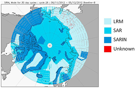
Figure 1. An example of the mode mask of Cryosat-2 for the Arctic Ocean for November 2012. The mask is dynamically changing with time. Faint blue regions means that data in LRM mode. Light blue is data in SAR and dark blue is data in SAR-in. Picture is from Cryosat-2 mission quality monitoring center (http://cryosat.mssl.ucl.ac.uk/qa/mode.php).

The previous version of DTU Arctic sea level dataset shows a questionable peak over the years 2002–2003, which corresponds to the first 2 years of ENVISAT, where particularly high sea level values are registered. A similar height anomaly is measured on global scale for the same period (Ablain et al., 2009; Figure 2). Currently this anomaly is still under investigation (ESA-CCI Sea level initiative, personal communication), and until it is understood we decided to update the version 3 of the Arctic time-series where we have replaced ENVISAT data with ERS-2 values along the period November 2002–July 2003. The comparison of the Arctic monthly averaged sea level over 66°N–82°N between version 2 and version 3 is displayed in Figure 3. The black curve represents the updated record. It can be noticed that a mean difference of 7.5 mm can be found between ERS-2 and ENVISAT (red curve) during the overlapping period.

FIGURE 2

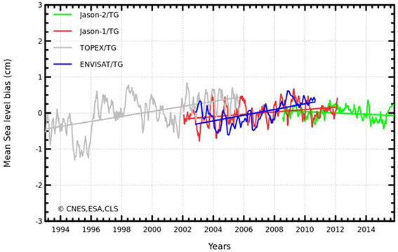
Figure 2. Difference between altimetry sea surface heights and tide gauges in situ measurements for four altimetry missions. Ambiguous values are observed for Envisat for 2002 and 2005 (Ablain et al., 2009).

FIGURE 3

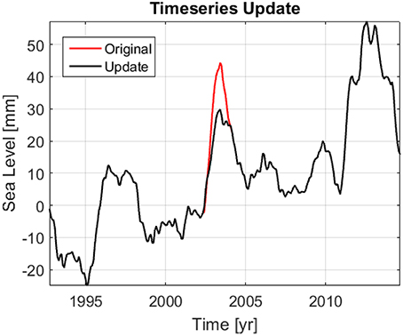
Figure 3. Version 3 of the Sea level record (black) based on ERS-2 compared with Version 2 containing Envisat (red) between 2002 and 2004.

Figure 4 shows the percentage of weekly observations available on the total amount of DTU Arctic sea level dataset. It is shown that within 20 years the largest number of observations is registered in the North Atlantic, while the availability of weekly data is down to around 20% between 120E and 120W (Cheng et al., 2015). This situation is related to the seasonal presence of ice in the interior of the Arctic Ocean. The irregular distribution of data both in space and time will impact on the interpretation and the subsequent computation of sea level trend budget closure. However, this result is still a huge improvement compared with standard edited datasets.

FIGURE 4

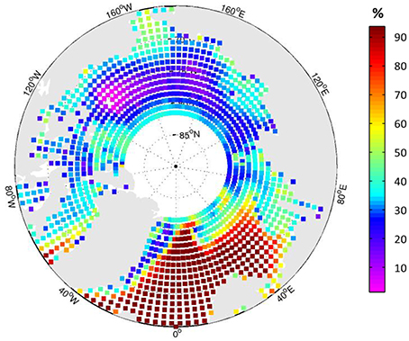
Figure 4. Percentage of weekly altimetric observations (b).

Grace Water Mass

For the subsequent regional Arctic sea level trend budget closure, monthly global Mascons products from GRCTellus JPL are used. The ocean data, also defined as Equivalent Water Thickness (EWT) are delivered as sampled on a one-by-one degree grids and covering the time period from 2003 to 2015 (Watkins et al., 2015). GRACE data are provided with associated errors.

Halo- and Thermo-steric Sea Level Data

Global gridded steric sea level anomalies with resolution one-by-one degree are provided by NOAA Ocean Heat and Salt content dataset. NOAA supplies separately thermo- and halo-steric values from https://www.nodc.noaa.gov/OC5/3M_HEAT_CONTENT/index.html. Both thermosteric and halosteric solutions are delivered every 3 months. Halosteric data at this temporal resolution are available for 2005 to present period, while thermosteric data cover the period 1955-present.

In Figure 5 the distribution of steric data used for NOAA grids are plotted for the common time span 2005–2015. High density is observed in the North Atlantic area and in the Beaufort Sea, while sparse data are available over Russia and Canadian Islands. It is expected that this irregular distribution varies also in time, meaning that for certain periods few or no data are available. The small number of direct observations will impact the estimation of steric sea level. Unfortunately, NOAA does not provide access to the model and associated spatial distribution of errors. Fortunately, the steric contribution over the analyzed period is relatively small and is not a dominating signal.

FIGURE 5

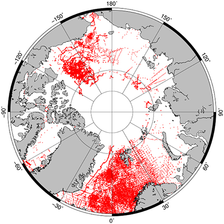
Figure 5. Distribution of steric values available for period 2005–2015.

Arctic Linear Sea Level Change (1993–2015)

To investigate the Arctic sea level trend in the region between 66°N and 82°N, the DTU Version 3 sea level dataset was used to compute the monthly mean sea level over the last 23 years as shown in Figure 6. From 2011 the monthly measurements (blue curve) register slightly higher annual fluctuations, which correspond to the fact that CRYOSAT-2 has more observations during leads in the winter period compared with conventional altimetry from ERS-1/ERS-2 and ENVISAT.

FIGURE 6

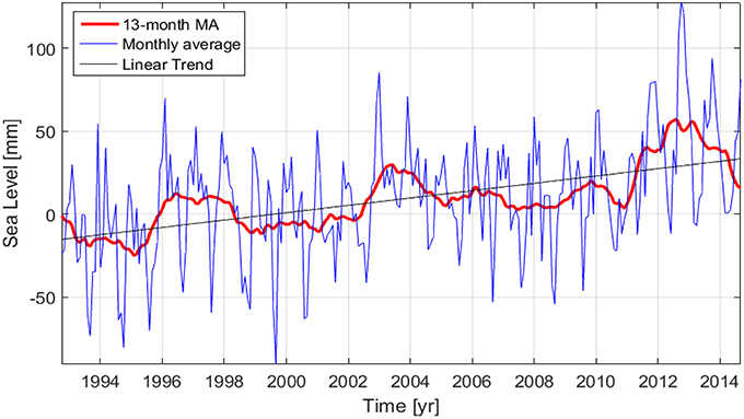
Figure 6. Regional sea level variations over 1993–2015. Monthly averaged values are shown in blue and 13-month averaged values are shown in red.

The regional sea level trend computed over the period 1993–2015 indicates an increase of 2.2 ± 1.1 mm/y, which is relatively consistent with the results obtained by Svendsen (2015) for the Arctic Ocean. The red curve represents the 1-year filtered sea level computed through a 13 term moving average (Hyndman, 2011). This highlights inter-annual variation in sea level which is as large as the sea level trend. Consequently estimation of linear sea level trend over shorter period is highly dependent on the chosen period.

A detailed view of spatial pattern of the linear sea level trend for period 1993–2015 is presented in Figure 7 with a resolution of 0.5° × 0.5°.

FIGURE 7

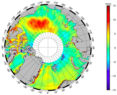
Figure 7. Spatial distribution of linear sea level trend for the period 1993–2015. An increase of 15 mm/y is observed in the Beaufort Sea. In the North Atlantic values corresponding to global sea level rise (Nerem et al., 2010) are found.

The trend pattern is dominated by a significant positive trend in the area of the Beaufort Sea, where an increase of almost 15 mm/y is registered. This is due to the Beaufort Gyre, a wind driven phenomenon that leads to freshwater accumulation (Rabe et al., 2011; Giles et al., 2012). In the northern part of the North Atlantic we observe regional sea level trend of 3–5 mm/years, which is comparable to what is seen by i.e., Nerem et al. (2010). Very close to the coast of Greenland the high sea level trend is questionable and can be attributed to the fact that few data exist during the ERS-1/ERS-2/ENVISAT period due to heavy sea ice coverage whereas in the same area Cryosat-2 provides a very narrow strip of SAR-in data.

Throughout most parts of the Russian Sector of the Arctic Ocean we only observe a relative small sea level trend of the order of 0–5 mm/year. This has to be further confirmed using tide gauges data in the region.

Regional Arctic Sea Level Trend Budget Closure

The sea level budget equation in its simplest form reads:

$\begin{array}{l}\Delta {\text{S}}_{\text{sl}}=\Delta {\text{S}}_{\text{mass}}+\Delta {\text{S}}_{\text{steric}}\hfill \end{array}$

Where ΔS_sl is the observed sea level, ΔS_mass is the ocean mass variation and ΔS_steric is the steric component. Both sea level and ocean mass variations are corrected for GIA. Smaller contributions due to inflow and outflow from the Arctic Ocean as well as sea level pressure variations with time should be accounted in the overall sea level trend budget.

Here a first attempt on regional basin scale for the Arctic Ocean is evaluated by comparing the updated sea level record with GRACE EWT values combined with the NOAA steric heights during the overlapping period 2005–2015. GRACE ocean mass variations are processed without accounting for the atmospheric pressure component. This correction is therefore applied using the ECMWF ERA-Interim model, and integrated according to Wunsch and Stammer (1997).

It is important to notice that in this first approach on sea level trend budget closure several crude assumptions are made as the prime purpose of the study is to perform a validation of the observed change in altimetry sea level over the period 2005–2015. First, it must be considered that there is a spatial limitation due to satellite coverage, and the central part of the Arctic Ocean (above 82°N) is not included. The same limitation can be found in steric observations, as mentioned in Section Halo- and Thermo-steric Sea Level Data. Secondly, the budget contains data from the Northern area of the Atlantic Ocean, which exchanges water with other parts of the Atlantic Ocean. This effect along with possible variations in the sea level pressure is not accounted for in this investigation. Finally, since NOAA steric data for 2005–2015 are provided with an interval of 3 months, both GRACE and altimetry time-series are also averaged according to the same temporal resolution before comparing these.

Table 1 shows the linear trend of the different components obtained from a least squares fit. The uncertainties are estimated from the least squares fit, as suggested in Leuliette (2014). For period 2005–2015 the altimetric record measures a sea level rise of 4.34 ± 2.44 mm/y, while GRACE EWT registers an increase of 3.85 ± 0.87 mm/y. The large error associated with the altimetry trend is most likely due to great standard deviation in sea level values along the time-series which again stems from large seasonal variation. The same consideration can be done for the steric components: large variation of data through time leads to high errors in slope, in particular for the thermosteric values.

TABLE 1

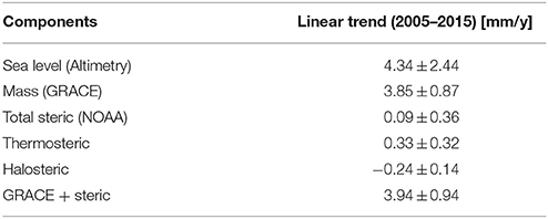
Table 1. Linear trend of sea level trend budget elements.

The sum of water mass and steric variations shows an increase in sea level of 3.94 ± 0.94 mm/y. This value falls within the error of altimetry trend, showing consistency between the results. The sea level trend budget based on seasonal values is closed with a difference of 0.4 ± 2.61 mm/y. This is believed to be an acceptable result from this first investigation considering the limitations described above.

In Figure 8 the 3-month averaged sea level budget contributions for the 2005-2015 period are shown. Large differences are observed between the single values of mass + steric and sea level, showing that on short timescales the budget is not closed. This is likely due to the poor and seasonal spatial sampling from altimetry and steric contribution of intra-annual signals.

FIGURE 8

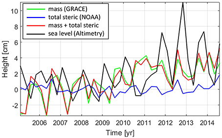
Figure 8. Three-month sea level variation from Altimetry (black) and EWT from GRACE (green), steric contribution (blue), and the sum of ocean mass (GRACE) with steric height (red). All values are in centimeters.

Larger values registered in sea level from 2010 and continuing into 2013 can be observed also with smaller fluctuations in GRACE (green curve), and its combination with the steric components (red curve). The larger fluctuations starting in 2010 can be subscribed to the fact that Cryosat-2 SAR altimetry provides far more data in the interior of the Arctic Ocean due to its improved ability to detect sea level in smaller leads in the ice. The sea level event during 2012–2013, could likely be associated with the recording melting in the Arctic Region as also seen on Greenland (Khan et al., 2015), but more research is needed.

Summary

In this study we have presented an improved version of the Arctic Ocean sea level record for the region 66°N–82°N covering the period 1993–2015. The dataset was modified to account for an unknown error in the ENVISAT data for the years 2002 and 2003, and it was updated with CRYOSAT-2 data until 2015. The record shows a total sea level rise of 2.2 ± 1.1 mm/y. The regional trend highlights a significant increase of 15 mm/y in the Beaufort Sea, corresponding to changes in the Beaufort Gyre. In the northern part of the North Atlantic we observe regional sea level trend of 3–5 mm/years, which is similar to what is seen by i.e., Nerem et al. (2010) for the global ocean.

With GRACE EWT products and NOAA steric models we have derived a first Arctic sea level trend budget closure for the period 2005–2015. Sea level trend of 4.4 mm/years were largely explained by similar trend in water mass derived from GRACE with a minor contribution from steric variations. This results in an acceptable sea level closure of 0.4 mm/y far within the errorbar of the altimetric sea level trend estimate. General agreement is found in the seasonal estimates between the altimetric records and the GRACE+steric combination, where a common increase is observed after 2010.

Author Contributions

All authors listed, have made substantial, direct, and intellectual contribution to the work, and approved it for publication.

Data

The various DTU Arctic sea level data can be found as along track data and as monthly gridded SLA anomalies for the Arctic Ocean through the DTU Space public portal: ftp://ftp.space.dtu.dk/pub/ARCTIC_SEALEVEL.

Conflict of Interest Statement

The authors declare that the research was conducted in the absence of any commercial or financial relationships that could be construed as a potential conflict of interest.

Acknowledgments

We would like to acknowledge different agencies for providing the datasets. Altimetry measurements are obtained from RADS at: http://rads.tudelft.nl/rads/rads.shtml. GRACE ocean data available at http://grace.jpl.nasa.gov. More information can be found in Chambers and Bonin (2012). The steric dataset is found in NOAA Global Ocean Heat and Salt Content section, on: https://www.nodc.noaa.gov/OC5/3M_HEAT_CONTENT/index.html, and ECMWF model for atmospheric pressure at sea level, retrieved from: http://www.ecmwf.int/en/research/climate-reanalysis/browse-reanalysis-datasets.

References

Ablain, M., Cazenave, A., Valladeau, G., and Guinehut, S. (2009). A new assessment of the error budget of global mean sea level rate estimated by satellite altimetry over 1993–2008. Ocean Sci. 5, 193–201. doi: 10.5194/os-5-193-2009

CrossRef Full Text | Google Scholar

Andersen, O. B., Knudsen, P., and Stenseng, L. (2015). “The DTU13 MSS (Mean Sea Surface) and MDT (Mean Dynamic Topography) from 20 years of satellite altimetry,” in International Association of Geodesy Symposia (Berlin; Heidelberg: Springer), 1–10. doi: 10.1007/1345_2015_182

CrossRef Full Text | Google Scholar

Andersen, O. B., and Scharroo, R. (2011). “Range and geophysical corrections in coastal regions: and implications for mean sea surface determination,” in Coastal Altimetry, eds S. Vignudelli, A. G. Kostianoy, P. Cipollini, and J. Benveniste (Berlin; Heidelberg: Springer), 103–145. doi: 10.1007/978-3-642-12796-0_5

CrossRef Full Text | Google Scholar

Chambers, D. P., and Bonin, J. A. (2012). Evaluation of Release-05 GRACE time-variable gravity coefficients over the ocean. Ocean Sci. 8, 859–868. doi: 10.5194/os-8-859-2012

CrossRef Full Text | Google Scholar

Cheng, Y., Andersen, O. B., and Knudsen, P. (2015). An improved 20-year Arctic Ocean altimetric sea level data record. Mar. Geod. 38, 146–162. doi: 10.1080/01490419.2014.954087

CrossRef Full Text | Google Scholar

Church, J. A., White, N. J., Konikow, L. F., Domingues, C. M., Cogley, J. G., Rignot, E., et al. (2011). Revisiting the Earth's sea-level and energy budgets from 1961 to 2008. Geophys. Res. Lett. 38:L18601. doi: 10.1029/2011GL048794

CrossRef Full Text | Google Scholar

Giles, K. A., Laxon, S. W., Ridout, A. L., Wingham, D. J., and Bacon, S. (2012). Western Arctic Ocean freshwater storage increased by wind-driven spin-up of the Beaufort Gyre. Nat. Geosci. 5, 194–197. doi: 10.1038/ngeo1379

CrossRef Full Text

Henry, O., Prandi, P., Llovel, W., Cazenave, A., Jevrejeva, S., and Stammer, D. (2012). Tide gauge-based sea level variations since 1950 along the Norwegian and Russian coasts of the Arctic Ocean: contribution of the steric and mass components. J. Geophys. Res. 117, C06023. doi: 10.1029/2011JC007706

CrossRef Full Text | Google Scholar

Hyndman, R. J. (2011). “Moving averages,” in International Encyclopedia of Statistical Science, ed M. Lovric (Berlin; Heidelberg: Springer), 866–869. doi: 10.1007/978-3-642-04898-2_380

CrossRef Full Text | Google Scholar

Khan, S. A., Aschwanden, A., Bjørk, A. A., Wahr, J., Kjeldsen, K. K., and Kjær, K. H. (2015). Greenland ice sheet mass balance: a review. Rep. Prog. Phys. 78:046801. doi: 10.1088/0034-4885/78/4/046801

PubMed Abstract | CrossRef Full Text | Google Scholar

Leuliette, E. (2014). Report on The Budget of Recent Global Sea Level Rise 2005-2013. Available online at: http://www.star.nesdis.noaa.gov/sod/lsa/SeaLevelRise/documents/NOAA_NESDIS_Sea_Level_Rise_Budget_Report_2014.pdf

Nerem, R. S., Chambers, D. P., Choe, C., and Mitchum, G. T. (2010). Estimating mean sea level change from the TOPEX and Jason altimeter missions. Mar. Geod. 33 (Suppl. 1), 435–446. doi: 10.1080/01490419.2010.491031

CrossRef Full Text | Google Scholar

Pavlov, V. K. (2001). Seasonal and long-term sea level variability in the marginal seas of the Arctic Ocean. Polar Res. 20, 153–160. doi: 10.1111/j.1751-8369.2001.tb00051.x

CrossRef Full Text | Google Scholar

Proshutinsky, A., Ashik, I. M., Dvorkin, E. N., Häkkinen, S., Krishfield, R. A., and Peltier, W. R. (2004). Secular sea level change in the Russian sector of the Arctic Ocean. J. Geophys. Res. 109, C03042. doi: 10.1029/2003JC002007

CrossRef Full Text | Google Scholar

Rabe, B., Karcher, M., Schauer, U., Toole, J. M., Krishfield, R. A., Pisarev, S., et al. (2011). An assessment of Arctic Ocean freshwater content changes from the 1990s to the 2006–2008 period. Deep Sea Res. Part I Oceanogr. Res. Papers 58, 173–185. doi: 10.1016/j.dsr.2010.12.002

CrossRef Full Text | Google Scholar

Scharroo, R., Leuliette, E. W., Lillibridge, J. L., Byrne, D., Naeije, M. C., and Mitchum, G. T. (2013). “RADS: Consistent multi-mission products,” in Proceedings of the Symposium on 20 Years of Progress in Radar Altimetry, (Venice: Eur. Space Agency Spec. Publ., ESA SP-710), 4.

Google Scholar

Stenseng, L. (2011). Polar Remote Sensing by CryoSat-type Radar Altimetry. Ph.D. thesis. National Space Institute, Technical University of Denmark.

Stenseng, L., and Andersen, O. B. (2012). Preliminary gravity recovery from CryoSat-2 data in the Baffin bay. Adv. Space Res. 50, 1158–1163. doi: 10.1016/j.asr.2012.02.029

CrossRef Full Text | Google Scholar

Svendsen, P. L. (2015). Arctic Sea Level Reconstruction. Ph.D. diss., Technical University of Denmark.

Tomczak, M., and Godfrey, J. S. (2003). Regional Oceanography: An Introduction, 2nd Edn. Delhi: Daya Publication.

Google Scholar

Volkov, D. L. (2014). Do the North Atlantic winds drive the nonseasonal variability of the Arctic Ocean sea level? Geophys. Res. Lett. 41, 2041–2047. doi: 10.1002/2013GL059065

CrossRef Full Text | Google Scholar

Volkov, D. L., and Landerer, F. W. (2013). Nonseasonal fluctuations of the Arctic Ocean mass observed by the GRACE satellites. J. Geophys. Res. Oceans 118, 6451–6460. doi: 10.1002/2013JC009341

CrossRef Full Text | Google Scholar

Watkins, M. M., Wiese, D. N., Yuan, D.-N., Boening, C., and Landerer, F. W. (2015). Improved methods for observing Earth's time variable mass distribution with GRACE using spherical cap mascons. J. Geophys. Res. Solid Earth 120, 2648–2671. doi: 10.1002/2014JB011547

CrossRef Full Text | Google Scholar

Wunsch, C., and Stammer, D. (1997). Atmospheric loading and the oceanic inverted barometer effect. Rev. Geophys. 35, 79–107.

Google Scholar