Statistical Analysis of the Acceleration of Baltic Mean Sea-Level Rise, 1900–2012

1. Introduction

Global mean sea-level has generally risen during the twentieth and twenty-first century due to the warming of the world oceans, melting of glaciers and polar ice-caps (Church and White, 2011; Church et al., 2011). The mean rate of global mean sea-level rise over this period has turned to be difficult to quantify exactly because the available sea-level data set in this period is not homogeneous, comprising a few tide-gauges records in the nineteenth century and the beginning of the twentieth century, and satellite altimetry in the twenty-first century with almost global coverage (Jevrejeva et al., 2008). The mean rate of sea-level rise has been estimated within an approximate range of 1.2 mm year⁻¹ (Hay et al., 2015) to 1.5–2.0 mm year⁻¹ (Hamlington and Thompson, 2015), whereas the most recent rates estimated from satellite altimetry indicate higher rates of the order of 3.1 mm year⁻¹ (Cazenave et al., 2014; Jevrejeva et al., 2014).

The projections of global sea-level rise by the end of the twenty-first century derived from the thermal expansion of the world ocean in global climate simulations, together with estimation of melting of land-locked ice indicate an upper range of sea-level rise close to 0.9 m relative to the mean sea-level of the twentieth century (Church et al., 2013; Clark et al., 2015). Therefore, the projections of global mean sea-level rise by 2100 imply an acceleration of its rate, since a linear extrapolation of the twentieth century rate, or even of the higher more recent rate derived from satellite altimetry, would yield a global mean sea-level rise of at least of the order of 30–40 cm by 2100.

In this study, we focus tide-gauge records of sea-level in the Baltic Sea with the goal of detecting an acceleration of the observed sea-level rise in this region. The Baltic Sea records offer the advantage of its unusual temporal and spatial coverage, many of them spanning the whole twentieth century and a few even longer, but unavoidably they can only provide information on regional sea-level. Global sea-level reconstructions offer a much wider coverage but they are constructed combining different sources of information, such as tide-gauges and satellite altimetry, and with a time varying level of spatial coverage. Thus, their use for detection of a still emerging and not totally clear signal in the observational period might be compromised by inhomogeneities (Church and White, 2011; Hamlington and Thompson, 2015).

An important question in the detection of acceleration in a climate record is precisely the definition of acceleration. Although velocity and acceleration in a kinematic context are precisely defined as the first and second second time derivative, respectively, the application of these definitions to discreet time series is not straight forward.

Similarly to the definition of linear trend in a stochastic process as a linear change trough time of its mean the acceleration could be defined as a non-linear increase through time of its mean. This non-linear increase can be quadratic or adopt a more complex functional form. Due to the generally limited length of sea-level time series and the high level of noise usually present in them, the detection of a distinctly non-linear increase of the mean of the underlying process is challenging unless the signal-to-noise ratio is high. In the context of sea-level records, several publications have reviewed some of the methods to estimate accelerations used in studies of sea-level rise (e.g., Visser et al., 2015).

Visser et al. (2015) discussed in detail and classifies 30 methods to estimate trends in time series, with some of them also applicable to estimate the acceleration. As stressed in that publication, there is no clear best method—as the different methods may display competing properties of estimation variance and bias, and the true value of the acceleration is not known. Here, we will apply three methods (augmented with some variants) to estimate the acceleration. These methods are intended to be physically motivated, as the estimate quantities that are very often computed to monitor the evolution of sea-level.

One estimation method (1) (Houston and Dean, 2011) computes the acceleration as the second order coefficient (multiplied by 2) of a second-order polynomial fit to a sea-level record. This estimation method is parametric, since it assumes a predetermined functional form for the acceleration. If the acceleration does not conform to this functional form, the detection of acceleration might be compromised (Haigh et al., 2014).

A second estimation method (2) of acceleration relies on the calculation of gliding linear trends over a multiyear period. These gliding trends represent the rate of sea-level rise over this limited period. An acceleration would be then detected if the rates of sea-level rise display long-term increase (or decrease) over time. This estimation method has been frequently used (Holgate, 2007; Visser et al., 2015), although the exact definition of “changes over time” varies in the different studies so far. Usually, acceleration is considered to be detected when the rate of rise compared in two different periods separated in time, for instance at the beginning and at the end of the record, are significantly different (Jevrejeva et al., 2008; Haigh et al., 2014). A slightly different variant of this method was applied by one meta-study (Spada et al., 2015), based on a collection of published analysis of sea-level rates covering different periods, established a regression between those estimated rates and the mean point in time that each study covers. The acceleration is then estimated as the tendency of the sea-level rate to increase over time, as found in that particular collection of analyses. We will also explore a similar definition in the present study.

A third estimation method (3) computes the annual increments of sea-level, i.e., the value of annual mean sea-level in a certain year minus the value of annual mean sea-level in the previous year, and estimate the acceleration as a the long-term tendency of those annual increments to become larger (or smaller) over time. This increase could be assumed to be linear in a first approximation, i.e., a long-term linear trend, and in theory can be estimated by ordinary linear regression on time.

Related to these estimation methods is the question of the attribution of any acceleration to external climate forcing, such as anthropogenic greenhouse gases (Slangen et al., 2016). We do not address this question in this study, but we note here that, for attribution purposes, the analysis of the decadal rates according to definition (2) would be the more adequate among these three definitions, since a detection and attribution study would be first focused on determining at which point in time the estimated rates of sea-level rise leave the range of fluctuations that may be considered “natural” within a stable climate (Haigh et al., 2014).

The computation of acceleration at the regional scale is also important beyond purely scientific reasons. A robust detection of acceleration and even an estimation of its value, can be used to provide a better range, based on available observations, of future sea-level rise in the next decades than the purely linear extrapolation of the more recent rate of rise, which could result in an underestimation of future sea-level rise. This information can be then incorporated in scientific assessments provided to regional planning agencies, although this approach would not cover any uncertainties due to new dynamics of the ice-sheets that may be triggered by future warming and that is not encapsulated in the observations until present.

In this study, we aim at detecting an acceleration of Baltic Sea-level analysing long records of the Baltic-Sea tide gauges applying these estimation methods.

The Baltic Sea is a semi-enclosed basin located at mid-to-high-latitudes in the Northern Hemisphere and strongly exposed to the atmospheric weather originating in the North Atlantic. For this reason, long-term trends of Baltic Sea-level, and changes thereof, may be influenced by other factors than the purely global sea-level rise due to global warming. The warming of the ocean water column has not been uniform over the globe and climate simulations also indicate a large spatial heterogeneity in the ocean warming (Church et al., 2004; Stammer et al., 2013; Slangen et al., 2014; Carson et al., 2015). Baltic-Sea level is strongly influenced by the westerly winds over the North Atlantic that push water from the North Sea into the Baltic Sea (Jevrejeva et al., 2005; Hünicke and Zorita, 2006; Barbosa, 2008; Bastos et al., 2013; Hünicke et al., 2015) rising Baltic Sea level. Thus, any long-term trends in internal modes of climate variability, like the North Atlantic Oscillation (NAO), will be also reflected in trends of sea-level (Calafat and Chambers, 2013). However, the influence of the NAO on Baltic Sea level is not spatially uniform due to the complex coastline of the Baltic Sea, with this influence being stronger in the North and East than in the South (Hünicke and Zorita, 2006). Other meteorological forcings (precipitation, run-off, local temperature) may also locally affect trends in Baltic-Sea level (Hünicke and Zorita, 2006).

The tide-gauges located in the North may be also influenced by sea-ice cover in winter. The melting of floating sea-ice, in contrast to floating pure water ice, may affect sea-level due to its lower salinity and temperature being lower than those of surrounding water (Jenkins and Holland, 2007; Shepherd et al., 2010). Another effect of diminishing ice cover in winter is a reduction of the missing values reported by the tide-gauges affected by sea-ice cover. Since the Baltic sea-level displays a clear annual cycle, this effect can spuriously affect the computed trends of sea-level trends and sea-level acceleration in those tide-gauges. The Bothnian Bay in the North is covered by sea-ice permanently for at least 150 days per year and the frequency and extent of sea-ice cover is diminishing in this area due to rising temperatures (Haapala et al., 2015).

In addition, the melting of polar-ice caps and land-glaciers also has a spatially heterogeneous fingerprint on regional sea-level due to the self-gravitational effect between land-ice and the ocean water masses (Mitrovica et al., 2001). For the Baltic Sea, the most important contribution from melting of land-ice stems from the Antarctic Ice sheets, whereas the contribution from Greenland is almost negligible—disregarding here the possible effect of Greenland melting on the circulation of the North Atlantic, which may also influence Baltic Sea level (Landerer et al., 2007). The time evolution of the melting of the Antarctic ice cap is still quite uncertain, with estimations of recent mass balance over the last few decades suggesting either sign (Zwally et al., 2015). Although higher temperatures over Antarctica will stimulate melting, these may also produce higher solid precipitation, so that the change in mass balance is a delicate difference between two uncertain quantities, at least in the recent decades. Therefore, the effect of the Antarctic contribution to Baltic Sea acceleration is also uncertain.

Finally, it is well-known that relative sea-level in the Baltic, as recorded by tide-gauges is subject to a very strong trend due to the Glacial Isostatic Adjustment (GIA), with relative sea-level falling in the North of the Baltic-Sea by about 10 mm⁻¹ and rising the South of the Baltic Sea by about 1 mm⁻¹ e.g., (Richter et al., 2012). The computation of acceleration is in theory not affected by the GIA as long as it is assumed that the effect of the GIA is linear within the time-scales analyzed here of about 100 years. However, the depression of the Earth crust caused by the ice load in the Last Glacial Maximum was of the order of several hundred meters. The current rate of recovery from this deformation is of the order of a few mm year⁻¹ and the acceleration estimated from tide-gauge records, as indicated later, is of the order of magnitude of tenths of μm year⁻². Therefore, an estimation of the possible effect of the GIA on the acceleration of relative sea-level is a priori justified and we will estimate this effect by using a simple physical model.

The total rise of sea-level in the Baltic sea by year 2100 has been recently projected at about 1 meter under the strongest emissions scenario RCP8.5 (Grinsted et al., 2015), which implies a very strong acceleration relative to the present rate of sea-level rise of 3.1 mm ⁻¹ (Stramska and Chudziak, 2013). All in all, the detection of acceleration of Baltic Sea level over several decades would support the future projections of increasing rates of sea-level rise. However, a lack of detection of acceleration can be due to multiple regional causes and would not necessarily disprove these future projections.

2. Data

We use Revised Local Reference tide-gauge data of long records of Baltic Sea level kindly provided by the Permanent Service for Mean Sea Level (PSMSL), 2016, “Tide Gauge Data,” (Retrieved 1 Nov 2015 from http://www.psmsl.org/data/obtaining/). These data have been profusely screened to detect inhomogeneities. We consider here all Baltic tide-gauges with time coverage starting no later than 1900, when the number of missing values is considerably reduced. A further selection rule of tide-gauges sets the limit of missing months in the records to 25% in the period 1900–2002, with the exception of two tide-gauges that include 27% of missing months. For the sake of completeness we include in the analysis some tide-gauges located also in the North Sea. We use annual means of sea-level until year 2012. Table 1 contains the list of PSMSL records included in this study and their starting and end years as used in this analysis.

TABLE 1

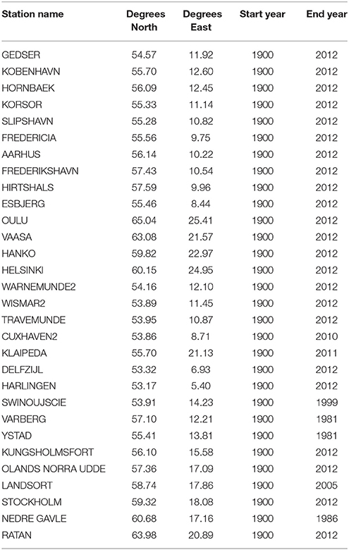
Table 1. List of stations from the Permanent Service for Mean Sea Level (PSMSL) used in this study together with their geographical location and start and end dates of the records used in this analysis (some stations provide longer records beyond this time range).

To test the statistical methods to detect the acceleration, we use the sea-level projections obtained from the suite of global climate models participating in the Climate Model Intercomparison Project version 5 (CMIP5) used by the Intergovernmental Panel on Climate Change (IPCC). This projections take into account the expansion of the ocean water column as simulated by the CMIP5 models, augmented by more uncertain estimations of land-ice melting (Carson et al., 2015). We use projections based on three different scenarios of atmospheric greenhouse gas concentrations, the so called Representative Concentration Paths RCP2.6, RCP4.5, and RCP8.5, labeled after their implied external radiative forcing in w m⁻² by year 2100.

We compute the globally averaged mean sea-level and the mean sea-level averaged over a geographical box in the North Atlantic (40W-0E; 30N-60N) of the mean of over all models (ensemble mean). The purpose of this choice is to test the power of the methods to detect the acceleration of sea-level rise under more controlled conditions, in a situation with low noise (ensemble mean) and high signal (future scenarios). These projections of sea-level intrinsically contain an acceleration of global sea-level rise, so that we can evaluate to what extent the statistical methods are able to detect this acceleration.

3. Methods

The estimation method (1), denoted in this study as pol₂, is based on the fit of a sea-level record to a time polynomial of order two:

$\begin{array}{ll}sl(t)=s{l}_0+bt+a{t}^2+ϵ(t)& (1)\end{array}$

where sl₀ is the initial sea level, b is the linear trend in sea level rise, ϵ is the sea level variability not explained by the polynomial, and 2a is the acceleration of sea level. The parameters sl₀, b, and a can be estimated by Ordinary Least Squares. The estimation uncertainties can also be directly derived from the theory of Ordinary Least Squares if ϵ is assumed to be gaussian white noise. If this condition is not fulfilled, more complex methods based on bootstrapping are required to obtain realistic estimation uncertainties.

In this study we will use a parametric bootstrap to estimate the uncertainties in the parameter a within the estimation method (1). After fitting the sea-level records to a second order polynomial in time, the residuals ϵ(t) are used to construct surrogate residual time series that display the same serial correlation properties. These surrogate residuals are added to the deterministic part of the statistical model sl₀+bt+at² and a new set of parameters is computed. This processes is repeated 10,000 times to obtain an empirical distribution of parameters.

The estimation method (2) to detect the acceleration relies on the computation of gliding linear trends over segments of the record. This record is denoted in the following as gt(t), where t is a year index, and the linear trend is computed over the interval (t − m, t + m). Most of the time in this study, gt(t) represents annual means, but part of the analysis was also conducted with seasonal (summer or winter) means. The choice of the length of the time window in years of these segments m is a compromise between the need of a stable estimation of the gliding linear trends and the number of independent segments allowed by the length of the total sea-level record. Since the second step in the computation of the acceleration is the estimation of the long-term trend of the gliding trends, the number of independent segments will also influence the stability of the estimation of the acceleration.

In this study, we have chosen to compute gliding linear trends of 11-year segments (m = 5). The results do not essentially change when varying this number within a reasonable range of 7 (m = 3) to 15 years (m = 7). Some studies have suggested a much longer length of the time window to compute the linear trends, as long as 40 years (m = 20), but this suggestion aims at estimating the acceleration as the mean difference between two periods, and establishing its statistical significance. Since here we estimate the acceleration as the long-term trend of the gliding trends, a larger number of independent degrees of freedom is desirable.

The third estimation method of the sea-level acceleration on computing the annual increments of an annual mean sea-level record sl(t) as inc(t) = sl(t) − sl(t − 1), where t is again a year index. The acceleration is then estimated as a long-term trend in the record of increments inc(t).

The estimation of the long-term trend in gt(t) or inc(t) can be carried out also another method different from Ordinary Linear Least Squares (OLS) regression. Here, we also computed the acceleration using as second non-parametric method, the Theil-Sen (TS) estimator (Schmith, 2008), to estimate the long-term trend. This estimator does not assume a linear functional dependency of the record over time, as ordinary linear regression does. It is based on the computation of the difference between all possible pairs in a record, say inc(t) − inc(t′), where t and t′ are two different years, with t occurring later than t′. The Theil-Sen estimator of the long-term trend is the sample median of all quantities $\frac{inc(t)-inc(t^{\prime })}{t-t^{\prime }}$.

Therefore, the acceleration estimators(2) and (3) can be implemented with two estimators of the long-term trend of gt(t) and inc(t). This yields four methods to estimate a final value of the acceleration, which will be denoted here as gt_ols, gt_ts, inc_ols, and inc_ts, following the convection gt = gliding trends, inc = annual increments, ols = ordinary least squares, and ts = Theil-Sen estimator, respectively.

The estimation of the uncertainties of the acceleration in the methods (2) and (3) are also obtained by bootstrapping. The records of gliding trends gt(t), and quite possibly also the record of increments inc(t) contain strong serial correlations, i.e., the individual samples are not independent. In the case of gt(t), this is particularly clear since the gliding trends are computed over overlapping time segments, so that in the computation of the value of gt(t) and the value of gt(t − 1) with m = 5 only two values of the original record sl are different. This serial correlation strongly hinders the estimation of the uncertainties in the long-term trend of gt(t) or inc(t) if only Ordinary Linear Least Squares regression of these records on the variable time were applied (Bos et al., 2014). The uncertainty bounds computed in this way would be too optimistic, since in reality the serial correlation of the record over long de-correlation length can give rise to spurious long-term trends, thus introducing a larger uncertainty in the estimation of the true trend. To avoid this pitfall, we use here a method based on the Monte Carlo generation of surrogate time series (Ebisuzaki, 1997). Within this method surrogate replicas of one record are produced that have the same serial correlation but otherwise are uncorrelated in time, as explained below.

Once a linear long-term trend in gt(t) or inc(t) has been estimated by linear regression on the variable time, a record of the regression residuals is stored. Thousand replicas of this residual record are generated by phase randomization and added to the original, but linearly detrended gt(t) or inc(t) record, thus obtaining thousand replicas of a theoretically trend-less record that contains residuals with the same serial correlation as the original record. The linear trends of the surrogate records are then estimated, providing an empirical distribution of sample trends. If the estimated trend in gt(t) or inc(t) is larger than the 95% quantile of this empirical distribution, the estimated long-term trend (acceleration) is claimed to be statistically significant.

4. Testing the Detection Methods Using Future Sea-Level Projections

Figure 1A displays the records of the ensemble mean of the global annual mean sea-level simulated by the CMIP5 ensemble of models driven by three scenarios of greenhouse gases atmospheric concentrations. As it is very well-known, the mean projection for all scenarios indicate a rising sea-level but with different magnitudes. As illustration of the possible acceleration of the mean sea-level rise, Figure 1B displays the corresponding gliding trends computed over 11-year segments gt(t), and Figure 1C displays the record of annual increments inc(t). The rates of sea-level rise estimated by these two methods show an increase with time, more clearly in the more pessimistic scenario RCP8.5, but not so clearly in the other two scenarios. In the scenario with smaller increase in radiative forcing, the rates of sea-level rise would even decelerate or remain nearly constant after 2020–2030.

FIGURE 1

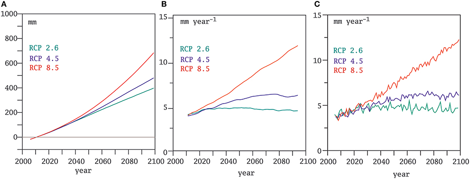
Figure 1. Global annual mean sea level from the ensemble mean of the CMIP5 models driven by three RCP greenhouse gas scenarios. (A) deviations from the 2006–2015 mean; (B) gliding trends computed over 11-year overlapping periods; (C) annual increments of the global annual mean sea-level.

This visual impression is confirmed by the numerical estimation of the acceleration based on the gt(t) and inc(t) records, as summarized in Table 2.

TABLE 2

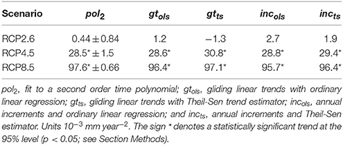
Table 2. Acceleration of global annual mean sea-level rise derived from the CMIP5 ensemble-mean driven by three Representative Concentration Paths scenarios, estimated in the period 2006–2099 using four estimation methods (see main text).

The values of the acceleration computed by the different methods are quite similar, supporting a robust estimation of its value, at least in this synthetic example in which the signal-to-noise ratio is high and averaging the global annual records over many models. Also, the accelerations detected in the scenarios RCP4.5 and RCP8.5 are statistically significant, corroborating the visual impression gained from Figure 1.

A more challenging test is to detect the acceleration not of the global mean sea-level but of the projected regional sea-level in the North Atlantic, a quantity more relevant for the analysis of the Baltic Sea acceleration. Figure 2 displays the simulated ensemble-mean annual sea-level (Figure 2A), its gliding trends (Figure 2B) and annual increments (Figure 2C) for the geographical region (40W-0E, 30N-60N) located in the North Atlantic. In this case, as expected, the records contain more regional noise, and the acceleration here, understood as a systematic increment in the rate of sea-level rise, is not visually detectable except for the more pessimistic scenario RCP8.5. Particularly noisy are the records of annual increments shown in Figure 2C. In this latter case, it becomes quite clear that any statistical method would struggle to detect a long term trend in the series of annual increments. This impression is supported by the numerical estimations of the acceleration contained in Table 3.

FIGURE 2

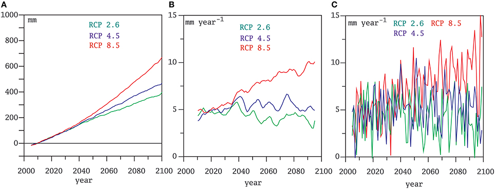
Figure 2. Annual mean sea level averaged over the North Atlantic (40W-0E;30N-60N) from the ensemble mean of the CMIP5 models driven by three RCP greenhouse gas scenarios. (A) deviations from the 2006–2015 mean; (B) gliding trends computed over 11-year overlapping periods; (C) annual increments of the average annual mean sea-level.

TABLE 3

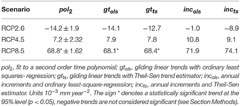
Table 3. Acceleration of North Atlantic annual mean sea-level rise derived from the CMIP5 ensemble-mean driven by three Representative Concentration Paths scenarios, estimated in the period 2006–2099 using four estimations methods (see main text).

The simulated sea-level rise, its rates and the acceleration estimated for the North Atlantic are smaller than for the global mean, which could be physically justified considering the projected cooling in this region due to a possible slow-down of the meridional overturning circulation in the North Atlantic. The further discussion of this point lies, however, outside the scope of this study, although it has to be borne in mind when discussing the acceleration of the Baltic sea-level during the twentieth century. More relevant here is the conclusion that the statistical method based on the annual increments turns to be in this case less powerful to detect a significant acceleration. Whereas the pol₂ and both methods based on gliding trends gs_ols and gs_ts indicate that the acceleration in the North Atlantic for the scenario RCP85 is statistically significant—also supported by the visual inspection of the time series shown in Figures 2A,B—the methods based on the annual increments inc_ols and inc_ts are not able to detect a statistically significant trend, even in the more pessimistic scenario RCP8.5.

We will, for the sake of brevity, show only the results obtained from the pol₂ and gt methods on the Baltic Sea tide-gauges records.

5. Acceleration of Baltic Sea Level

Figure 3 shows the estimated sea-level acceleration of the annual mean sea-level in 30 tide-gauges from the PSMSL records, estimated with the pol₂ and the two gliding trends methods (gt_osl and gt_ts). The numerical values with their estimated uncertainties are included in Table 4. The spatial patterns are similar, with a range of spatial correlations between all three patterns ranging between r = 0.70 and r = 0.75. The value of the acceleration averaged over all stations is also similar in the three cases, with 12.2 mm × 10⁻³ year⁻² with the pol₂ method, 13.6 × 10⁻³ mm year⁻² with the gt_ols method, and 17.7 × 10⁻³ mm year⁻² obtained with the gt_ts method. Just as illustration of the consequences of an average acceleration of this magnitude, assuming that it is distributed uniformly over time and continues unchanged in the future, this value of the acceleration implies an additional sea-level rise relative to a simple linear extrapolation of the present rise of about 65 mm in 100 years for the all-stations-average. Very few of the individual accelerations computed for the individual tide-gauge records turns to be statistically significant applying any of the gliding trend methods.

FIGURE 3

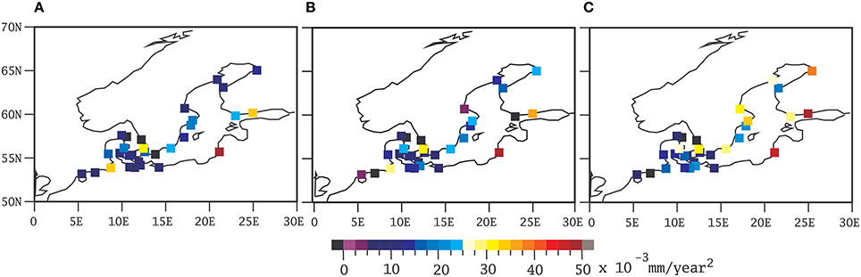
Figure 3. Acceleration of the annual mean sea-level in the Baltic Sea tide-gauges estimated in the period 1900–2012 by the methods (A) pol₂, (B) gt_ols, and (C) gt_ts. See Table 4.

TABLE 4

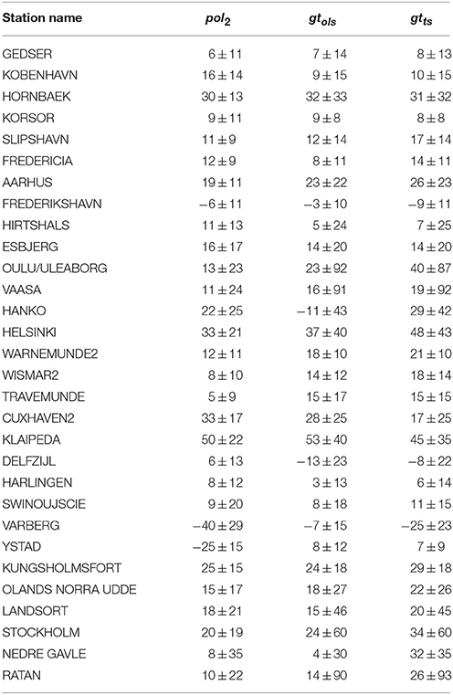
Table 4. Acceleration of the annual mean sea-level in the Baltic Sea tide-gauges and their estimated 95% uncertainty range derived by the methods pol₂, gt_ols, and gt_ts in 10⁻³ mm year⁻² in the period 1900–2012.

The spatial patterns of accelerations do not show a very clear geographical structure. However, there is a tendency for larger accelerations to be found at the tide-gauges located toward the North and the East. This tendency is more clearly displayed in Figure 4. This figure shows the scatter plot of the annual (and also winter and summer for reasons discussed later) accelerations estimated with the gt_ols method as a function of geographical distance from the point 0W, 55N. The scatter plots also include the regression lines and their 95% uncertainty range. These scatter plots indicate a large scatter around the regression lines, but all three confirm the visual impression from Figure 3.

FIGURE 4

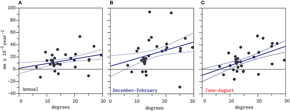
Figure 4. Acceleration of the annual (A), winter (B), and summer (C) mean sea-level in the Baltic Sea tide-gauges estimated in the period 1900–2012 by the methods gt_ols as a function of their distance to the geographical point 0W, 55N. The plots include the regression lines estimated by Ordinary Least Squares and their 95% uncertainty range.

As mentioned in the introduction, there are several spatially heterogeneous factors that affect Baltic Sea level and that could blur a spatially homogeneous patterns of acceleration. To check whether this local and regional noise can be filtered by computing an indicator of the spatial mean of Baltic Sea level, the all-stations-average time series has been computed and is displayed in Figure 5A, along with their record of decadal gliding trends in Figure 5B. Note that, since the magnitudes of the long-term trends caused by the GIA are spatially very heterogeneous, the individual tide-gauge records shown in Figure 4A have been previously linearly detrended and the deviations from their long-term mean also calculated, before computing the all-stations-average. This indicator of Baltic mean sea-level is not strictly well defined because the spatial coverage of the tide-gauges is not uniform: many stations in this set are clustered in the South -East of the Baltic Sea and the some in the basins connecting the North and the Baltic Seas. Also, the time correlation between the individual annual sea-level records is on average about 0.6, although there are pairs of tide-gauges that are correlated as low as 0.35. This means that it is difficult to compute a representative annual index of regional mean sea-level based on the available tide-gauges in this region.

FIGURE 5

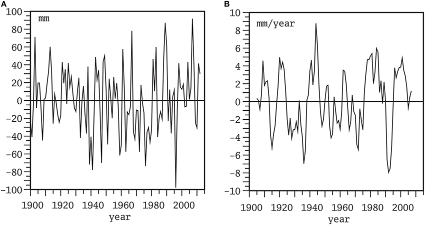
Figure 5. (A) All-stations-average of annual mean sea-level derived from the PSMSL tide-gauge show in Figure 3 in the period 1900–2012. (B) Its gliding trends computed over 11-year overlapping periods.

Nevertheless, the all-stations-average record (Figure 5A) may be illustrative of the variations of Baltic Sea level through time in the twentieth and twenty-first centuries. The highest decadal gliding trends (Figure 5B) have been attained around 1945, in agreement with similar calculations based on the Warnemünde tide-gauge (Richter et al., 2012) The acceleration, estimated as the long-term ordinary-least-squares trend (method gt_ols) of the decadal gliding trends is positive and attains a value of 14.5 × 10⁻³ mm year⁻². This value is close to the average of the individual accelerations computed for each tide-gauge (Figure 5A). This acceleration, though positive, is not statistically significant at the 95% level (p = 0.12). In contrast, most of the individual accelerations lie below the 95% significance level. Averaging over all stations, therefore, is able to filter out some noise, resulting in a marginally significant signal. This signal, however, remains weak, as illustrated in a barely discernible long-term trend in Figure 5B.

Very similar results are obtained with the gt_ts method to estimate the acceleration of the average record.

5.1. Influence of the Glacial Isostatic Adjustment

The spatial pattern of accelerations of relative sea-level in the Baltic Sea region suggests that tide-gauges located at higher latitudes may be experiencing stronger accelerations. The question arises as to whether this pattern could also be influenced by the GIA, as tide-gauges in the North are also subject to stronger relaxation velocities of the Earth's crust. In the following, we briefly estimate a possible order of magnitude of the effect of the GIA on acceleration.

The GIA is caused by the back-relaxation of the Earth's crust to the deformation caused by the load of land-ice during the last glacial period. The peak of the glacial period, the Last Glacial Maximum, was reached about 20,000 years ago and the de-glaciation in Fennoscandia was almost complete about 8000 years ago. The Earth's crust started rebounding after the ice load was released, pushed by the viscous rebalancing of the material in the Earth's mantle. It can be assumed that this GIA-related relaxation can be described by a simple exponential model:

$\begin{array}{ll}A(t)=A_0(1-e^{-t/\tau })& (2)\end{array}$

where t is time, A₀ is the maximum depression caused by the load of the ice-sheets and τ is a the typical viscous relaxation time. A plausible value for τ in this simple model would be of the order of 5000 years (Wieczerkowski et al., 1999), although the exact value is not critical for this simple estimation.

The acceleration of the crust $\frac{{\text{d}}^{2}A}{\text{d}{t}^2}$ is then proportional to its velocity $\frac{\text{d}A}{\text{d}t}$:

$\frac{{\text{d}}^{2}A(t)}{\text{d}{t}^2}=\frac{-1}{\tau }\frac{\text{d}A(t)}{\text{d}t}(3)$

The relative sea-level would experience the same magnitude of acceleration but with reversed sign, and thus present a pattern of acceleration reminiscent of the spatial pattern estimated here. In the North of the Baltic sea, where the GIA velocity is of the order of 10 mm year⁻¹, the GIA-related acceleration would amount to about 0.002 mm year⁻². This magnitude, therefore, seems to be small compared with the estimated accelerations displayed in Figure 3 which are one order of magnitude larger than the GIA-related acceleration estimated with this simple model. Although the GIA may contribute to the acceleration, it is likely not the whole explanation according to this simple model.

5.2. Role of Ice Cover

The formation and melting of floating sea-ice cover may also influence sea-level (Jenkins and Holland, 2007; Shepherd et al., 2010). With warming proceeding through the last decades, the ice cover in the Baltic Sea has been systematically reduced (Haapala et al., 2015). Since ice cover in winter time is more relevant for those tide-gauges located at higher latitudes, the melting of sea-ice could in principle also influence the estimation of acceleration. Another reason by which sea-ice may influence the estimation of coastal sea-level is the annual cycle of Baltic sea level (Hünicke and Zorita, 2008) together with the number of reported missing values. Baltic Sea level generally displays a maximum during wintertime, more clearly so at its northern than at the southern coasts. If sea-ice cover at the coast hinders the tide-gauge measurement, a diminishing sea-ice cover in recent decades would increase the relative weight of wintertime measurements in the annual means, leading to an artificial increase in the reported annual mean sea-level and potentially to an apparent acceleration of annual mean sea level. To test this possibility, we have also computed the accelerations with the gt_ols method for the winter (December through February) and summer (June through August) seasons. The results are depicted in Figure 6.

FIGURE 6

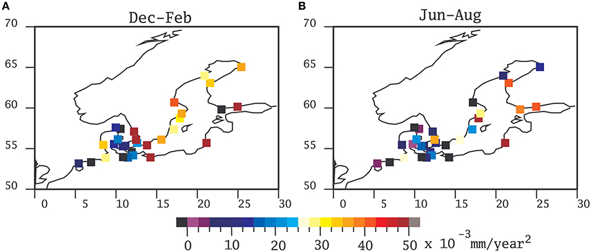
Figure 6. Acceleration of the annual mean sea-level in the Baltic Sea tide-gauges estimated in the period 1900–2012 in wintertime (A) and summertime (B) by the method gt_ols.

The spatial pattern of acceleration derived from the winter and summer data still display a tendency for higher values at higher latitudes and longitudes although the summer pattern is now more tilted in the east-west direction. This tendency was also visible in Figures 4B,C. In addition, the two most northern tide-gauges display in summertime a rather small acceleration. It seems, therefore, that the influence of the diminishing ice coverage would not explain the spatial patterns of acceleration in the Baltic although it may have some influence.

6. Concluding Remarks

Within the caveats explained in the introduction, the statistical methods used here fail to detect a statistically significant acceleration in the Baltic Sea area since 1900, which can be due to the still small magnitude of he acceleration paired with a high random sea-level variability at the regional scale.

Nevertheless, the computed individual accelerations in the Baltic Sea are mostly positive and the all-stations-mean almost attains the level of statistical significance. Its magnitude is nevertheless small. The implied increase by year 2100 over a purely linear extrapolation of the present rate would yield an additional increase of sea-level of few centimeters by year 2100.

We have adopted a definition of acceleration as a systematic increase of the rates of sea-level. This definition is not equivalent to other definitions of acceleration, more focused on the detection of “unusual” values, i.e., the comparison between recent rates and historical rates of sea-level rise. However, the adoption of this latter definition would also wrestle to claim an unusual rate of sea-level in the very last decades. The rates computed around year 2000 are indeed among the highest of the whole record, but they are not the absolute maximum (Figure 5B, see also Richter et al., 2012).

Unfortunately, global climate models lack the sufficient spatial resolution to realistically represent the Baltic Sea. Simulations with coupled regional climate models of the Baltic Sea would be very useful to ascertain if the acceleration of sea-level is also detectable in climate simulations, although it has to be borne in mind that all the subtle processes that may influence the long-term evolution of Baltic Sea level may not be realistically represented in these models, for instance, the connection to the North Sea or the dynamics related to sea-ice cover (Hordoir et al., 2015).

Author Contributions

All authors listed, have made substantial, direct and intellectual contribution to the work, and approved it for publication.

Conflict of Interest Statement

The authors declare that the research was conducted in the absence of any commercial or financial relationships that could be construed as a potential conflict of interest.

Acknowledgments

This study is part of the Cluster of Excellence Integrated System Analysis and Prediction (CLISAP), funded by the German Science Foundation, and of the Earth System Science Program for the Baltic Sea region (Baltic Earth). We thank Mark Carson of the Center für Erdsystemforschung und Nachhaltigkeit (CEN) of the University of Hamburg (Germany) for kindly providing the sea-level data of the CMIP5 simulation ensemble. We also thank the Permanent Service for Mean Sea Level (PSMSL) in Liverpool (UK) for proving an excellent data infrastructure. The manuscript benefited from very helpful comments from the reviewers.

References

Barbosa, S. M. (2008). Quantile trends in Baltic sea level. Geophys. Res. Lett. 35, L22704. doi: 10.1029/2008GL035182

CrossRef Full Text | Google Scholar

Bastos, A., Trigo, R., and Barbosa, S. (2013). Discrete wavelet analysis of the influence of the North Atlantic Oscillation on Baltic Sea level. Tellus A 65:20077. doi: 10.3402/tellusa.v65i0.20077

CrossRef Full Text | Google Scholar

Bos, M., Williams, S., Araújo, I., and Bastos, L. (2014). The effect of temporal correlated noise on the sea level rate and acceleration uncertainty. Geophys. J. Int. 196, 1423–1430. doi: 10.1093/gji/ggt481

CrossRef Full Text | Google Scholar

Calafat, F., and Chambers, D. (2013). Quantifying recent acceleration in sea level unrelated to internal climate variability. Geophys. Res. Lett. 40, 3661–3666. doi: 10.1002/grl.50731

CrossRef Full Text | Google Scholar

Carson, M., Köhl, A., Stammer, D., A. Slangen, A. B., Katsman, C. A., van de Wal, R. S. W., et al. (2015). Coastal sea level changes, observed and projected during the 20th and 21st century. Clim. Change 134, 269–281. doi: 10.1007/s10584-015-1520-1

CrossRef Full Text | Google Scholar

Cazenave, A., Dieng, H.-B., Meyssignac, B., von Schuckmann, K., Decharme, B., and Berthier, E. (2014). The rate of sea-level rise. Nat. Clim. Change 4, 358–361. doi: 10.1038/nclimate2159

CrossRef Full Text | Google Scholar

Church, J. A., Clark, P. U., Cazenave, A., Gregory, J. M., Jevrejeva, S., Levermann, A., et al. (2013). Sea-level rise by 2100. Science 342, 1445–1445. doi: 10.1126/science.342.6165.1445-a

PubMed Abstract | CrossRef Full Text | Google Scholar

Church, J. A., Gregory, J. M., White, N. J., Platten, S. M., and Mitrovica, J. X. (2011). Understanding and projecting sea level change. Oceanography 24, 130–143. doi: 10.5670/oceanog.2011.33

CrossRef Full Text | Google Scholar

Church, J. A., and White, N. J. (2011). Sea-level rise from the late 19th to the early 21st century. Surv. Geophys. 32, 585–602. doi: 10.1007/s10712-011-9119-1

CrossRef Full Text | Google Scholar

Church, J. A., White, N. J., Coleman, R., Lambeck, K., and Mitrovica, J. X. (2004). Estimates of the regional distribution of sea level rise over the 1950-2000 period. J. Clim. 17, 2609–2625. doi: 10.1175/1520-0442(2004)017<2609:EOTRDO>2.0.CO;2

CrossRef Full Text | Google Scholar

Clark, P. U., Church, J. A., Gregory, J. M., and Payne, A. J. (2015). Recent progress in understanding and projecting regional and global mean sea level change. Curr. Clim. Change Rep. 1, 224–246. doi: 10.1007/s40641-015-0024-4

CrossRef Full Text | Google Scholar

Ebisuzaki, W. (1997). A method to estimate the statistical significance of a correlation when the data are serially correlated. J. Clim. 10, 2147–2153.

Google Scholar

Grinsted, A., Jevrejeva, S., Riva, R. E. M., and Dahl-Jensen, D. (2015). Sea level rise projections for northern Europe under RCP8.5. Clim. Res. 64, 15–23. doi: 10.3354/cr01309

CrossRef Full Text | Google Scholar

Haapala, J. J., Ronkainen, I., Schmelzer, N., and Sztobryn, M. (2015). “Recent change—sea ice,” in Second Assessment of Climate Change for the Baltic Sea Basin, ed The BACC II Author Team (Cham: Springer International Publishing), 145–153.

PubMed Abstract

Haigh, I. D., Wahl, T., Rohling, E. J., Price, R. M., Pattiaratchi, C. B., Calafat, F. M., et al. (2014). Timescales for detecting a significant acceleration in sea level rise. Nat. Commun. 5:3635. doi: 10.1038/ncomms4635

PubMed Abstract | CrossRef Full Text | Google Scholar

Hamlington, B. D., and Thompson, P. R. (2015). Considerations for estimating the 20th century trend in global mean sea level. Geophys. Res. Lett. 42, 4102–4109. doi: 10.1002/2015GL064177

CrossRef Full Text | Google Scholar

Hay, C. C., Morrow, E., Kopp, R. E., and Mitrovica, J. X. (2015). Probabilistic reanalysis of twentieth-century sea-level rise. Nature 517, 481–484. doi: 10.1038/nature14093

PubMed Abstract | CrossRef Full Text | Google Scholar

Holgate, S. J. (2007). On the decadal rates of sea level change during the twentieth century. Geophys. Res. Lett. 34:L01602. doi: 10.1029/2006gl028492

CrossRef Full Text | Google Scholar

Hordoir, R., Axell, L., Löptien, U., Dietze, H., and Kuznetsov, I. (2015). Influence of sea level rise on the dynamics of salt inflows in the Baltic Sea. J. Geophys. Res. Oceans 120, 6653–6668. doi: 10.1002/2014JC010642

CrossRef Full Text | Google Scholar

Houston, J. R., and Dean, R. G. (2011). Sea-level acceleration based on US tide gauges and extensions of previous global-gauge analyses. J. Coast. Res. 27, 409–417. doi: 10.2112/JCOASTRES-D-10-00157.1

CrossRef Full Text | Google Scholar

Hünicke, B., and Zorita, E. (2006). Influence of temperature and precipitation on decadal baltic sea level variations in the 20th century. Tellus A 58, 141–153. doi: 10.1111/j.1600-0870.2006.00157.x

CrossRef Full Text | Google Scholar

Hünicke, B., and Zorita, E. (2008). Trends in the amplitude of Baltic Sea level annual cycle. Tellus A 60, 154–164. doi: 10.1111/j.1600-0870.2007.00277.x

CrossRef Full Text | Google Scholar

Hünicke, B., Zorita, E., Soomere, T., Madsen, K. S., Johansson, M., and Suursaar, Ü. (2015). “Recent change—sea level and wind waves,” in Second Assessment of Climate Change for the Baltic Sea Basin, ed The BACC II Author Team (Cham: Springer International Publishing), 155–185.

Jenkins, A., and Holland, D. (2007). Melting of floating ice and sea level rise. Geophys. Res. Lett. 34:L16609. doi: 10.1029/2007GL030784

CrossRef Full Text | Google Scholar

Jevrejeva, S., Moore, J., Grinsted, A., Matthews, A., and Spada, G. (2014). Trends and acceleration in global and regional sea levels since 1807. Glob. Planet. Change 113, 11–22. doi: 10.1016/j.gloplacha.2013.12.004

CrossRef Full Text | Google Scholar

Jevrejeva, S., Moore, J., Woodworth, P., and Grinsted, A. (2005). Influence of large-scale atmospheric circulation on European sea level: results based on the wavelet transform method. Tellus A 57, 183–193. doi: 10.1111/j.1600-0870.2005.00090.x

CrossRef Full Text | Google Scholar

Jevrejeva, S., Moore, J. C., Grinsted, A., and Woodworth, P. L. (2008). Recent global sea level acceleration started over 200 years ago? Geophys. Res. Lett. 35:L08715. doi: 10.1029/2008GL033611

CrossRef Full Text | Google Scholar

Landerer, F. W., Jungclaus, J. H., and Marotzke, J. (2007). Regional dynamic and steric sea level change in response to the IPCC-A1B scenario. J. Phys. Oceanogr. 37, 296–312. doi: 10.1175/JPO3013.1

CrossRef Full Text | Google Scholar

Mitrovica, J. X., Tamisiea, M. E., Davis, J. L., and Milne, G. A. (2001). Recent mass balance of polar ice sheets inferred from patterns of global sea-level change. Nature 409, 1026–1029. doi: 10.1038/35059054

PubMed Abstract | CrossRef Full Text | Google Scholar

Richter, A., Groh, A., and Dietrich, R. (2012). Geodetic observation of sea-level change and crustal deformation in the Baltic Sea region. Phys. Chem. Earth 53, 43–53. doi: 10.1016/j.pce.2011.04.011

CrossRef Full Text | Google Scholar

Schmith, T. (2008). Stationarity of regression relationships: application to empirical downscaling. J. Clim. 21, 4529–4537. doi: 10.1175/2008JCLI1910.1

CrossRef Full Text | Google Scholar

Shepherd, A., Wingham, D., Wallis, D., Giles, K., Laxon, S., and Sundal, A. V. (2010). Recent loss of floating ice and the consequent sea level contribution. Geophys. Res. Lett. 37:L13503. doi: 10.1029/2010GL042496

CrossRef Full Text | Google Scholar

Slangen, A., Carson, M., Katsman, C., van de Wal, R., Köhl, A., Vermeersen, L., et al. (2014). Projecting twenty-first century regional sea-level changes. Clim. Change 124, 317–332. doi: 10.1007/s10584-014-1080-9

CrossRef Full Text | Google Scholar

Slangen, A. B. A, Church, J. A., Agosta, C., Fettweis, X., Marzeion, B., and Richter, K. (2016). Anthropogenic forcing dominates global mean sea-level rise since 1970. Nat. Clim. Change 6, 701–705. doi: 10.1038/nclimate2991

CrossRef Full Text | Google Scholar

Spada, G., Olivieri, M., and Galassi, G. (2015). A heuristic evaluation of long-term global sea level acceleration. Geophys. Res. Lett. 42, 4166–4172. doi: 10.1002/2015GL063837

CrossRef Full Text | Google Scholar

Stammer, D., Cazenave, A., Ponte, R. M., and Tamisiea, M. E. (2013). Causes for contemporary regional sea level changes. Annu. Rev. Mar. Sci. 5, 21–46. doi: 10.1146/annurev-marine-121211-172406

CrossRef Full Text | Google Scholar

Stramska, M., and Chudziak, N. (2013). Recent multiyear trends in the Baltic Sea level. Oceanologia 55, 319–337. doi: 10.5697/oc.55-2.319

CrossRef Full Text | Google Scholar

Visser, H., Dangendorf, S., and Petersen, A. C. (2015). A review of trend models applied to sea level data with reference to the “acceleration-deceleration debate.” J. Geophys. Res. Oceans 120, 3873–3895. doi: 10.1002/2015JC010716

CrossRef Full Text | Google Scholar

Wieczerkowski, K., Mitrovica, J. X., and Wolf, D. (1999). A revised relaxation-time spectrum for Fennoscandia. Geophys. J. Int. 139, 69–86.

Google Scholar

Zwally, H. J., Li, J., Robbins, J. W., Saba, J. L., Yi, D., and Brenner, A. C. (2015). Mass gains of the Antarctic ice sheet exceed losses. J. Glaciol. 61, 1019–1036. doi: 10.3189/2015JoG15J071

CrossRef Full Text | Google Scholar