Atlantic Advection Driven Changes in Glacial Meltwater: Effects on Phytoplankton Chlorophyll-a and Taxonomic Composition in Kongsfjorden, Spitsbergen

Introduction

Phytoplankton dynamics in the coastal Arctic are shaped by extreme seasonality in irradiance. During the polar night phytoplankton experience a prolonged period of darkness. The return of light marks the start of the spring bloom (Berge et al., 2015). Arctic sea ice cover in spring and summer months has declined for several decades, also around the Svalbard archipelago (Stroeve et al., 2007). Reduced sea ice cover enhances phytoplankton irradiance exposure and pelagic phytoplankton productivity in vast parts of the Arctic Ocean (Arrigo and van Dijken, 2015). Density differences due to melting sea ice or glacial meltwater stabilize the water column, allowing phytoplankton to maintain their position and form highly productive surface blooms. Stratification is associated with diatom blooms in the marginal ice zones (Syvertsen, 1991; Perrette et al., 2011). However, strong stratification can also lead to nutrient limitation and changes phytoplankton taxonomic composition and biomass (Li et al., 2009). In the absence of stratification, convection and strong winds can mediate deep turbulent mixing of the water column that can reduce phytoplankton irradiance exposure and reduce phytoplankton growth (Townsend et al., 1994).

The Greenland and Barents Sea experience inflow of Atlantic water with variable heat content (Lien et al., 2013). Kongsfjorden (79°N, 11°40′E) and the West coast of Spitsbergen are influenced by warm saline Atlantic water of the West Spitsbergen Current (WSC) and colder less saline Arctic water of the East Spitsbergen Current (ESC) that mix on the continental shelf (Cottier et al., 2005). As a result, fjords on the West coast of Spitsbergen can experience highly variable sea water temperature conditions. The temperature of the WSC showed an increasing trend from 1997 to 2010 (Beszczynska-Möller et al., 2012). Recent increases in advection of Atlantic water in Kongsfjorden have been attributed to changes in density by warming of the WSC, reduced drift ice in the ESC, and changes in wind direction (Cottier et al., 2007, 2010).

Advection of warm Atlantic water in winter and early spring can prevent sea ice formation in Kongsfjorden. The changing conditions in Kongsfjorden have been suggested to affect phytoplankton productivity and taxonomic composition (Hegseth and Tverberg, 2013; Kubiszyn et al., 2014). These changes may arise from multiple causes. Warmer Atlantic water may harbor different phytoplankton species and a more boreal grazer community (Willis et al., 2008). Furthermore, transition from an ice covered to an open fjord in winter can change the starting population by affecting growth conditions of pelagic phytoplankton. An open fjord in spring can promote convective mixing, but advection of Atlantic water at the surface can also reduce the depth of convective mixing (Hegseth and Tverberg, 2013). Moreover, increasing sea water temperature promotes glacial melting, which affects the strength and timing of stratification as well as turbidity (Hop et al., 2002; Luckman et al., 2015; Bartsch et al., 2016). In the absence of melting sea ice, melt water from marine terminating glaciers is the dominant source of fresh water in Kongsfjorden (MacLachlan et al., 2007), producing a steep fresh water gradient during spring and summer (Piquet et al., 2014).

Kongsfjorden spring blooms show considerable variability in timing and composition, typically consisting of diatoms and Phaeocystis pouchetii, whereas small flagellates dominate during the nutrient limited post bloom period (Iversen and Seuthe, 2011; Hegseth and Tverberg, 2013; Piquet et al., 2014). Phytoplankton abundance and composition affect carbon fluxes to pelagic and benthic higher trophic levels (Bhatt et al., 2014). In addition, this eventually affects carbon storage in the ocean. The present study aims to improve our understanding of the processes that affect phytoplankton biomass and composition in Kongsfjorden. We investigated an annual time series of phytoplankton pigment samples from the 2013 to 2014 polar night, spring bloom, and following post bloom. Furthermore, we investigated effects of Atlantic water advection on stratification, phytoplankton biomass, and composition during the spring bloom from April to June (2014) by sampling two stations in the glacial meltwater gradient. The goal was to understand the effects of Atlantic water advection on stratification and phytoplankton biomass and composition dynamics. We specifically address the hypothesis that in the absence of sea ice, glacial melt water is the dominant factor that defines the timing and composition of the phytoplankton spring bloom.

Methods

The research was conducted at 3 locations in Kongsfjorden, Spitsbergen (79°N, 11°40′E), covering the period from October 2013 to December 2014. Samples were collected at the ferry box of the AWIPEV Underwater Fjord Observatory in Ny Ålesund (Fischer et al., 2016) that collects water from 11 m depth (100 m off shore) in Kongsfjorden (Figure 1). Samples were taken over weekly intervals, whereas sampling frequency was increased from April to June ranging from daily to twice a week, with 24 samples being collected during this period. Seawater samples (4–8 L) were filtered on 47 mm GF/F (Whatman) using 0.2 bar overpressure, snap frozen in liquid nitrogen, and stored at −80°C. The samples were analyzed for phytoplankton pigments by High Performance Liquid Chromatography (HPLC) as described below. During the 2013–2014 polar night and following spring bloom (October 2013–June 2014), temperature from 11 m depth was obtained from a SBE38 temperature sensor (Sea Bird Electronics) from which daily averages were calculated. Average daily air temperature (2 m) was calculated from the BSRN measurement platform in Ny Ålesund.

FIGURE 1

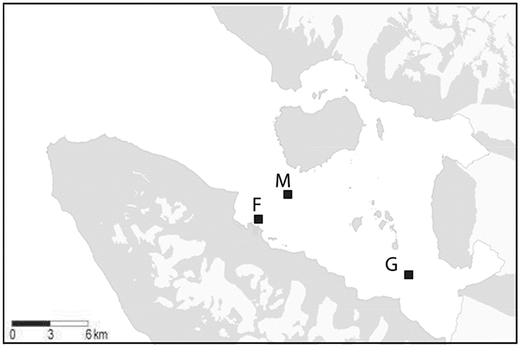
Figure 1. Map of Kongsfjorden with the sampling locations mid fjord: M, glacier: G, ferry box: F. Source: Basisdata/NP_Basiskart_Svalbard_WMS (http://geodata.npolar.no/bruksvilkar/), with stations included as GPS coordinates.

In addition, regular sampling (19–28 times) was performed by boat from April to June 2014 at two stations in Kongsfjorden: “Glacier station” (G), located in front of the Kronebreen glacier (inner Kongsfjorden) and “Midfjord station” (M), located in central Kongsfjorden (Figure 1). Vertical profiles of the water column were collected at station G (50 m) and M (100 m) using a CTD (SBE 19 plus, Sea-Bird Electronics) equipped with sensors for PAR (Licor, Sea-Bird Electronics), fluorescence (Wetstar), and turbidity (ECO NTU, Wetlab). From these profiles, salinity, temperature, potential density, and turbidity at 5, 25, and 50 m depth were extracted. Potential density differences in excess of 0.005 kg m⁻³ between surface (5 m) and 50 m depth were considered indicative for stratification (Kara et al., 2000). Irradiance attenuation (K_d) was calculated by linear regression of log transformed PAR data. The euphotic zone (defined as the depth interval down to 0.1% irradiance) was calculated as: Z_eu (m) = − ln (0.001)/K_d.

Samples were collected at 5, 25, and 50 m depth at both stations using a 24 L Niskin bottle. The samples were kept cold and stored in darkness until processing in the lab. Pigment samples were obtained by mild vacuum filtration (0.2 bar) of 4–10 L seawater on 47 mm GF/F (Whatman) filters. Afterwards, filters were snap frozen in liquid nitrogen and stored at −80°C until HPLC pigment analysis. Five mL subsamples were filtered (0.2 μm Acrodisc, Pall) for nutrient analysis and frozen at −20°C (nitrate and nitrite, phosphate, ammonium) or stored at 4°C (silicate) until analysis using a Bran and Luebbe QuAAtro auto analyzer to determine dissolved inorganic phosphate, ammonium, nitrate, and nitrite, and silicate at the NIOZ, The Netherlands.

Subsamples for microscopy (100 mL) were fixed with 1.5 mL Lugol's iodine solution and stored dark at 4°C until analysis using an Olympus IMT-2 inverted microscope (Utermöhl technique, Edler and Elbrächter, 2010). This procedure was conducted at 20 samples collected between April 26 and June 10, 2014 at station M (n = 10) and G (n = 10) to observe the general phytoplankton composition (presence of diatoms, flagellates, Phaeocystis, dinoflagellates, cryptophytes). The phytoplankton was not enumerated in these samples and the results are not shown. We report phytoplankton abundance and the abundance of large heterotrophic dinoflagellates and ciliates of 4 samples collected at 5 m depth (station M: May 5, 10, and 28, station G: May 28).

Phytoplankton Pigment and CHEMTAX Analysis

Filters were freeze dried for 48 h and pigments were extracted using 90% acetone (v/v) for 48 h (4°C, darkness). Pigments were separated by HPLC (Waters 2695) with a Zorbax Eclipse XDB-C8 column (3.5 μm particle size), using the method of Van Heukelem and Thomas (2001), modified after Perl (2009). Detection was based on retention time and diode array spectroscopy (Waters 996) at 436 nm. Pigments were manually quantified using standards for all used pigments (DHI lab products). The absolute and relative abundances of phytoplankton groups were assessed by CHEMTAX analysis of pigments, using the steepest descent algorithm (version 1.95) (Mackey et al., 1996). Pigments were partitioned among 7 groups (based on microscopic observations): diatoms (fucoxanthin), prasinophytes (chlorophyll b, neoxanthin, prasinoxanthin), haptophytes (19′butanoloxyfucoxanthin, fucoxanthin, 19′hexanoloxyfucoxanthin, chlorophyll c3), pelagophytes (19′butanoloxyfucoxanthin, fucoxanthin, chlorophyll c3), chrysophytes (19′butanoloxyfucoxanthin, fucoxanthin, 19′hexanoloxyfucoxanthin, chlorophyll c3), dinoflagellates (peridinin), and cryptophytes (alloxanthin). CHEMTAX results of the haptophyte and pelagophyte sub-groups were pooled (these groups showed similar dynamics) and will be denoted as “haptophytes.” Ferry box samples with chl-a below 0.01 mg m⁻³ were excluded for CHEMTAX analysis because many accessory pigments became undetectable in these dilute samples. Ferry box samples collected during the nutrient replete spring bloom (n = 40) and those collected during the nutrient depleted post bloom (n = 24) were grouped in separate bins. Non-stratified samples of station M (5, 25, and 50 m; n = 24) were grouped in a single bin. Stratified samples of M and G were analyzed in two depth bins: 5 and 25 m, (n = 52), and 50 m (n = 26). We used identical low light acclimated initial pigment ratios for all bins (Supplement Table 1A). All pigments were allowed to vary during CHEMTAX analysis (chl-a: 100%, other pigments: 500%). Final pigment ratios are shown in Supplement Table 1B.

Data Analysis

Analysis of the ferry box data series (October 2013–December 2014) and the data series of stations M and G (April–June 2014) were performed separately. Annual distribution of 2014 phytoplankton chl-a and taxonomic composition was assessed for weekly averaged ferry box samples (chl-a n = 81, CHEMTAX n = 64). Exponential growth rates of chl-a during the nutrient replete spring bloom were calculated by fitting log transformed chl-a vs. time with a linear function.

During the spring bloom we used linear correlation (Pearson Product Moment) to investigate relationships between environmental data and non-linear correlation (Spearman Rank Order) when investigating relationships between environmental and biological data for dates with a complete biological and physical data set of stations M and G. Correlations were considered significant at p < 0.05.

Results

Annual Cycle 2014 (Ferry Box)

The underwater observatory recorded declining sea water temperatures from October 2013 (maximum 5.60°C) to the beginning of January 2014 (minimum 0.67°C, Figure 2A). After January 16 temperature increased to 3.36°C (first inflow event, Figure 2A). This was preceded by elevated air temperature. Sea water and air temperature declined from the end of February to the beginning of April (minimum 0.32 and −16.55°C, respectively), and increased from April onwards (second inflow event, Figure 2A). Chl-a concentrations declined by two orders of magnitude during the polar night from October 20 to February 23, 2014 (Figure 2B). The 2014 ferry box time series showed average concentrations of 0.023 ± 0.018 mg chl-a m⁻³ during the polar night (samples from October 20 to December 27, 2014, and from October 20, 2013 to February 20, 2014, n = 21). Increasing chl-a coincided with the return of light, light dose correlated linearly with chl-a from February 20 to April 12 (r_s = 0.97, n = 10). Peak concentrations of up to 4.9 mg m⁻³ were observed on June 5. This coincided with depletion of nitrate, dissolved inorganic phosphate, and silicate (Figure 3A, Supplement Figure 1). The non-stratified period (February 20 to May 2, see below) showed lower chl-a based exponential growth rates (Table 1) and overall lower chl-a concentrations (average 0.15 ± 0.90 mg m⁻³) as compared to the stratified spring bloom period (May 5–June 5, average 2.4 ± 2.0 mg m⁻³). The nutrient depleted post bloom period (June 9–October 20) showed lower average chl-a (0.60 ± 0.36 mg m⁻³). Chl-a increased from July 14 to August 25 (average 0.79 ± 0.17), before declining during the polar night.

FIGURE 2

Figure 2. (A) Daily averaged sea water temperature at the ferry box inlet (11 m) from October 2013 to June 2014 (left y axis) and air temperature in Ny Ålesund at 2 m. The numbers 1 and 2 indicate Atlantic advection events. (B) Ferry box chlorophyll-a concentration and daily PAR dose (photosynthetically active radiation, 400–700 nm) in Ny Ålesund from October 2013 to June 2014.

FIGURE 3

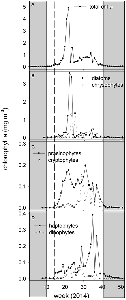
Figure 3. Weekly averaged chlorophyll-a concentration of the 2014 ferry box samples (A) total chl-a, (B) chl-a of diatoms and chrysophytes, (C) chl-a of prasinophytes and cryptophytes, and (D) chl-a of haptophytes and dinoflagellates, derived by CHEMTAX analysis. The vertical dashed line marks the transition from non-stratified to stratified conditions. The shaded area indicates the polar night.

TABLE 1

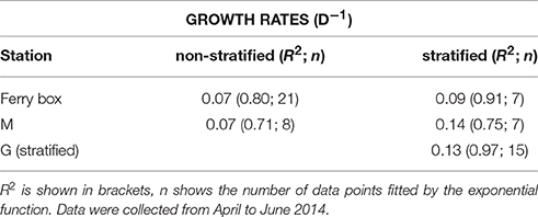
Table 1. Exponential growth rates (d⁻¹) of phytoplankton chlorophyll-a concentration (5 m) of the ferry box data series, and of stations mid fjord (M), and glacier (G), under stratified and non-stratified conditions.

CHEMTAX pigment analysis revealed shifts in phytoplankton taxonomic groups during the spring bloom and the following nutrient depleted post bloom (Figure 3). Diatom and chrysophyte chl-a peaked on June 5, representing 68 and 26% of the spring bloom chl-a concentration peak at the ferry box, respectively. Prasinophyte chl-a peaked prior to the spring bloom peak (May 6) and during the post bloom (July 31) period at a maximum relative abundance of 41% of chl-a. The post bloom period (June 9–October 20) showed a decline in relative abundance of diatoms and chrysophytes, averaging of 25 and 26% of chl-a in June and July. Peridinin-containing dinoflagellates and cryptophyte chl-a peaked in July, at a maximum of 14 and 18% of chl-a, respectively. Chrysophytes increased to 40% of chl-a in August, whereas haptophytes peaked in early September (maximal 40% of chl-a). Flagellated photosynthetic phytoplankton declined in relative abundance during the polar night, with diatoms increasing in relative abundance (>90% of chl-a).

Spring 2014 (Stations M and G)

Physicochemical Data

Marked differences in salinity and temperature were observed over time and at depth between stations M and G during the spring of 2014 (Figure 4). Salinity at 25 and 50 m of station M (35.08 ± 0.01) was higher than at station G (34.94 ± 0.05). Potential density at station M of these depths was higher than at station G up to May 5. Temperature at station M (5 m average: 2.10 ± 0.70°C) was higher than at station G (5 m average 0.54 ± 0.99°C), and increased from April 11 to 14, and from May 5 onwards (Figure 4). Water column temperature at station G increased from April to June. Surface temperature (5 m) at M (May 5–May 28) and G (April 14–May 28) to was typically lower compared with 50 m.

FIGURE 4

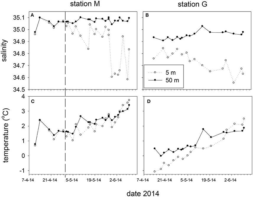
Figure 4. Salinity (A,B) and temperature (C,D) at 5 and 50 m depth at station M and G between April and June 2014. The vertical dashed line marks the transition from non-stratified to stratified conditions at station M.

The temperature and salinity increase at station M from April 11 to 14 was followed by a period with minimal potential density differences (no stratification) between 5 and 50 m up to May 2. During this period temperature and salinity showed similar and significant positive correlations at 5, 25 and 50 m (ρ = 0.97, 0.96, 0.95). After stratification of station M due to decreasing surface salinity (May 5 and onwards), this relationship was not observed at 5 m, and became weaker at 25 and 50 m. Station G was always stratified from April 14 to June 10 (Figure 5). Stratification strength correlated inversely with surface salinity (ρ = −0.96, −0.95 for G and M, respectively). Stratification strength increased with surface temperature at station G and M (ρ = 0.93, 0.64, respectively). In May, stratification strength increased at M, and differences between M and G became minimal by the end of May. At station G an inverse correlation was found between temperature and salinity at 5 m (ρ = −0.78), whereas positive correlations were observed at 25 and 50 m (ρ = 0.96, 0.94) up to May 10.

FIGURE 5

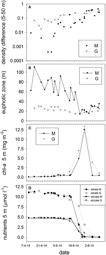
Figure 5. Stratification strength as differences in potential density between 5 and 50 m (A), (B) euphotic zone depth, (C) surface chlorophyll-a (5 m), and (D) nitrate and silicate concentrations (5 m) at stations M and G from April to June 2014.

Irradiance attenuation was strong at station G, resulting in a euphotic zone of 23 ± 5 m that showed little change over time (Figure 5). The euphotic zone of station M was on average 70 ± 19 m up to May 20, and declined to 24 ± 7 m afterwards. Surface turbidity correlated positively with the attenuation coefficient K_d of M and G (ρ = 0.65). Between April and June, turbidity in the upper 25 m was on average 0.53 ± 0.37 at station M whereas this was 2.43 ± 0.91 for station G (not shown).

Surface (5 m) nitrate (10.78 ± 0.37 μM), phosphate (0.65 ± 0.06 μM, Supplement Figure 2) and silicate (4.75 ± 0.05 μM) concentrations were high from April to early May (Figure 5), and showed little variability with depth (Supplement Figure 2). Surface (5 m) nutrient concentrations declined steeply during the second half of May, and were close to the detection limits by the end of May at stations G and M (average phosphate: 0.019, nitrate:0.06, and silicate: 0.08 μM). In June, average surface N:P (nitrate: phosphate) ratios were 3.6 and 2.4 for stations M and G, respectively. Prior to May 7, N:P ratios were on average 16.72 ± 0.89 and 18.02 ± 2.25 at M and G, respectively. Ammonium increased at station M and G from 0.15 ± 0.07 to 0.34 ± 0.06 μM at 5 m from April 14 to June 10. Ammonium increased to 1.35 ± 0.28 μM at 25 and 50 m depth (Supplement Figure 2).

Phytoplankton Chlorophyll-a

Chlorophyll-a concentrations at stations M and G were low (0.026 mg m⁻³) in early April (Figure 5). Chl-a at station M was uniformly distributed over the water column from April 9 to May 7, and increased in the upper 25 m in May. Chl-a (5 m) was on average 28% higher at M compared to G during the non-stratified period (April 9–May 2), whereas it was on average (26%) lower than that at G after stratification (May 5–May 28). Surface chl-a (5 m) showed an exponential increase over time, peaking on May 28 (>10 mg m⁻³) at both stations (Figure 5). Chl-a based growth rates were higher at station G as compared to station M (Table 1). Prior to stratification of station M (April 11–May 2) the growth rate was ~50% lower than at station G. Chl-a based growth at stations G and M was similar after stratification. Surface chl-a declined to 0.6 mg m⁻³ in June.

Phytoplankton Composition

Taxonomic composition at station M and G showed differences in early spring (April–May, Figure 6). At station M diatoms were on average 31 ± 18% of chl-a from April 14 to May 16, and increased to 72 ± 14% on May 28. Diatoms comprised a high fraction of chl-a at station G between April and June (average 5 m: 71 ± 13%, Figure 6). Absolute diatom chl-a was on average 2.2-fold higher at G than at M during April–May 15 (Figure 6). During the same period flagellates (chl-a of haptophytes, prasinophytes, cryptophytes, dinoflagellates, and chrysophytes, combined) were 2.3-fold higher at station M than at G (Figure 6). During the stratified period, differences in absolute flagellates chl-a were 10% between M and G. Haptophyte relative abundance at station M declined from 34 ± 2.1% (April 14) to 4.0 ± 4.5% of chl-a (May 28). At station G haptophytes were 17 ± 4.1% of chl-a up to May 10 and declined to 4.0 ± 4.1% afterwards. Relative abundance of prasinophytes at M increased from April 9 (4%) to May 2 (34 ± 1%), and declined toward the end of May (Figure 6). At station G prasinophytes increased to 17 ± 1.6% of chl-a on May 10. Cryptophytes increased from April to May 16 from to 5.9% at station M, but were < 1% of chl-a at station G. The contribution of chrysophytes to chl-a was variable, ranging from 0 to 30% and 0 to 16% at station M and G, respectively. Peridinin-containing dinoflagellates were on average 1.6 and 0.4% of chl-a at M and G respectively (not shown). The spring bloom chl-a peak (May 28) was dominated by diatoms (72 and 85% of chl-a at M and G, respectively).

FIGURE 6

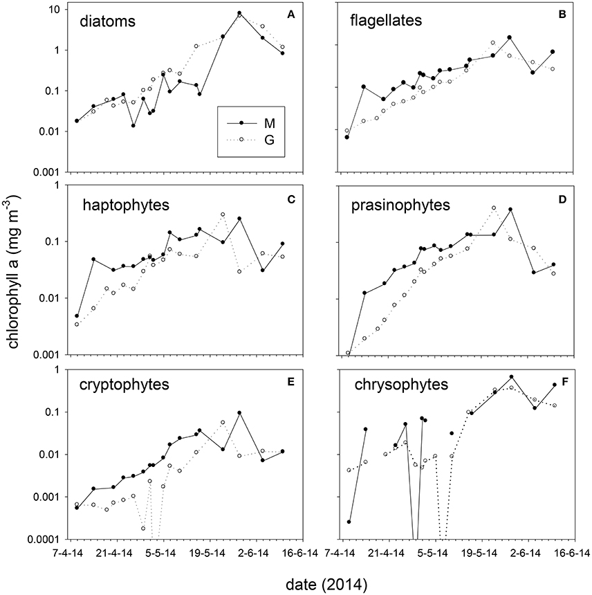
Figure 6. Absolute chlorophyll-a concentration (average 5, 25 m) of taxonomic groups at stations M and G from April to June 2014. (A) diatoms, (B) total flagellates (prasinophytes, haptophytes, chrysophytes, cryptophytes, and dinoflagellates combined), (C) haptophytes, (D) prasinophytes, (E) cryptophytes, and (F) chrysophytes. Note the difference in scale between graphs.

Relative abundances of haptophytes, diatoms, prasinophytes, and cryptophytes showed the strongest correlations with physical variables (Table 2). Relative abundance of haptophytes, prasinophytes, cryptophytes at station M and G (5, 25, and 50 m) showed positive correlations with surface salinity (r_s = 0.76, 0.66, 0.59) and euphotic zone depth (r_s = 0.76, 0.55, 0.54). Surface density showed positive correlations with haptophytes and prasinophytes (r_s = 0.72, 0.65). Relative abundance of haptophytes, prasinophytes, and cryptophytes showed an inverse correlation with stratification strength (r_s = −0.75, −0.58, −0.45). Relative abundance of diatoms at station M and G (5, 25, and 50 m) showed inverse correlations with surface salinity (r_s = −0.77), surface density (r_s = −0.67), and euphotic zone depth (r_s = −0.73). Relative abundance of diatoms showed a positive correlation with stratification strength (r_s = 0.66). Relative abundance of dinoflagellates correlated significantly with temperature (r_s = 0.70), and surface temperature (r_s = 0.67). All reported r_s-value were significant at p < 0.05.

TABLE 2

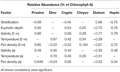
Table 2. Correlation coefficients of Spearman rank order correlation between relative abundance of prasinophytes, dinoflagellates, cryptophytes, chrysophytes, diatoms, and haptophytes at station M and station G (5, 25, 50 m) between April 14 and June 10, and stratification strength, euphotic zone depth, surface salinity, temperature, and potential density (5 m), and salinity, temperature, and potential density at actual depth (a); (n = 102).

Microscopy (Stations M and G)

Light microscopy revealed small (~2 μm) and larger (5–10 μm) flagellates dominating station M during the first half of May (Table 3). The larger flagellates (10 μm) were most likely Dictyocha speculum (Chrysophyceae). Small flagellates (~2 μm) were most likely Micromonas sp. (Prasinophyceae). Diatoms were rare in these samples. However, the peak of the bloom (May 28) was dominated by diatoms (mostly Chaetoceros sp., and Thalassiosira sp.) at stations M and G. At station M significant numbers of small flagellates were still observed, whereas these were less abundant at station G. Tintinnids (Ciliates) increased at station M, whereby concentrations were 8-fold higher compared to G during the peak of the bloom. Large heterotrophic dinoflagellates were also higher at M as compared to G.

TABLE 3

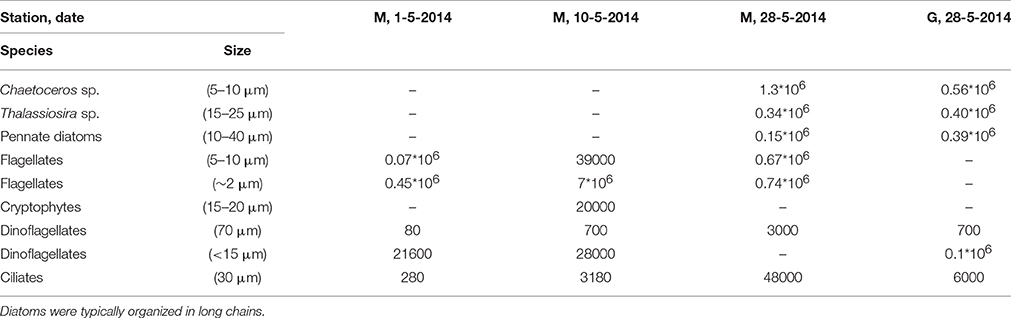
Table 3. Cell counts (cells l⁻¹) of dominant phytoplankton and ciliates of four samples of station M (3) and G (1) in Kongsfjorden obtained by light microscopy.

Discussion

Atlantic advection was observed during 2013–2014 polar night (underwater observatory) and spring (underwater observatory, CTD) in central Kongsfjorden. Atlantic water interrupted winter cooling of the fjord, with a temperature of 3°C at 11 m depth detected as early as January. Together with relatively high air temperature this prevented sea ice formation in 2014. Atlantic advection was episodic in early spring, followed by a period of cooling. During the second Atlantic advection event in April–May a salinity and temperature gradient was observed in the fjord, expanding from central to inner Kongsfjorden over time. Similar patterns were reported for Adventfjorden in 2014 (Wiedmann et al., 2016). The density of the intruding Atlantic water was higher than that of the inner fjord, resulting in advection at depth. This increased the temperature of the inner fjord, thereby promoting melting of marine terminating glaciers from below. The Atlantic water was the only heat source available during the 2014 spring bloom. The seasonally increasing contribution of air temperature and downward radiation became apparent by warming of the stratified surface layer in June. The fresh water influx of glacial melting induced stratification in inner Kongsfjorden. Stratification strength near the glacier correlated with water temperature, and was comparable in magnitude to that reported during sea ice mediated stratification in central Kongsfjorden (Hodal et al., 2012). Melt water driven stratification expanded from the inner fjord toward central Kongsfjorden in early May. Prior to stratification central Kongsfjorden showed deep convective mixing (April–May 2) due to surface cooling and strong wind, with surface nutrient concentrations close to the maximal concentrations reported for Kongsfjorden after winter (Hop et al., 2002; Piquet et al., 2014). The 2014 spring bloom peak in central Kongsfjorden occurred after glacial melt water driven stratification. The spring bloom peak was late compared to recorded Kongsfjorden spring bloom phenology from the last decade, which can be as early as April (Hegseth and Tverberg, 2013). Atlantic advection created a spatial and temporal gradient of stratification and light availability in the fjord in April and May. The glacial melting in the stratified inner fjord coincided with sediment discharge, resulting in a high turbidity and a shallow euphotic zone during spring bloom formation.

Chl-a based growth rates showed exponential growth from April to the end of May in the inner fjord. These growth rates were two times higher compared to those from central Kongsfjorden (April–May 16). Despite high water transparency in central Kongsfjorden, vertical mixing may have reduced phytoplankton light exposure due to mixing below the euphotic zone. This may have delayed the development of a surface bloom in central Kongsfjorden, whereas light limitation from glacial sediment influx may have reduced growth in the inner fjord. Furthermore, phytoplankton composition was different between the two locations during early spring. Early spring phytoplankton in central Kongsfjorden consisted mostly of flagellated phytoplankton (prasinophytes, haptophytes, cryptophytes, chrysophytes), whereas the inner fjord phytoplankton was dominated by diatoms. Therefore, the growth rates may reflect differences in community composition between the two locations. Previous research indicated that years with Atlantic advection during the spring bloom were characterized by increased abundance of the haptophyte P. pouchetii (Hegseth and Tverberg, 2013). Haptophyte pigments and Phaeocystis cells or colonies were not abundant during the 2014 spring bloom. Nevertheless, inverse correlations with stratification strength, and positive correlations with surface salinity, and euphotic zone depth suggest a link between haptophytes and the Atlantic water influenced central Kongsfjorden. Prasinophytes and cryptophytes showed similar links to Atlantic water characteristics. Vader et al. (2015) provided evidence for the continuous presence of Micromonas pusilla and P. pouchetii in the Arctic and Atlantic water surrounding Spitsbergen during the polar night. In contrast, relative abundance of diatoms showed an inverse relationship with surface salinity, euphotic zone depth, and a positive correlation with stratification strength. These relationships reflect the spatial distribution of the phytoplankton taxonomic groups and water masses (possibly due to introduction of haptophytes by Atlantic advection and diatoms of local origin) rather than the conditions that cause these differences. Overall, these relationships also point to the importance of stratification in shaping phytoplankton composition during the spring bloom. How stratification changed phytoplankton species composition remains unknown. Stratification at central Kongsfjorden did not cause immediate changes in the phytoplankton composition and chl-a based growth rates. Pronounced changes were observed 10 days after stratification of station M, and appeared to be caused by expansion of the low salinity surface layer with a diatom bloom that was initiated at the inner fjord. Apart from influencing phytoplankton light exposure and nutrient concentrations, stratification also affects concentration driven processes such as top down control (Behrenfeld, 2010). Chl-a based growth rates during the spring bloom were roughly 2–4 times lower as compared to those from cultured Arctic phytoplankton species, suggesting significant losses (due to grazing or viral lysis). Ciliates (30 μm) and large dinoflagellates were the most abundant grazers in our samples and were higher at station M compared to G during the peak of the bloom. These groups were previously shown to have a high potential to control small phytoplankton in Kongsfjorden (Seuthe et al., 2011). In addition, diatom resting stages can be suspended in the water column by deep mixing (Hegseth and Tverberg, 2013). Therefore, multiple factors influenced by stratification can potentially affect phytoplankton composition during the spring bloom.

We used pigments and CHEMTAX to assess changes in phytoplankton taxonomic composition. Light microscopy was used to select the taxonomic groups included in CHEMTAX and to verify the observed patterns such as the difference in abundance of diatoms at station M and G. Dicyocha speculum (Chrysophyceae) flagellates were occasionally observed in considerable numbers in microscopy samples from M and G during the 2014 spring bloom. Diatoms and chrysophytes are difficult to distinguish using CHEMTAX because both groups share high fucoxanthin to chl-a ratios, a feature that can also be observed in some haptophyte groups (Higgins et al., 2011). In addition chrysophytes share pigments with haptophytes. Furthermore, the presence of additional taxonomic groups in the 2014 ferry box data cannot be excluded as there were no microscopy samples of the ferry box time series. Therefore, the presented CHEMTAX based composition should be viewed as a crude estimates. Apart from errors related to CHEMTAX, microscopic identification is difficult for small flagellated phytoplankton groups. Moreover, it is difficult to distinguish between pigmented and non-pigmented dinoflagellates in Lugol's iodine fixed samples. Nevertheless, CHEMTAX calculations matched microscopy observation from station M and G reasonably well. This suggests that pigment samples provided useful taxonomic information of Kongsfjorden phytoplankton.

The ferry box time series identified spring as the most dynamic part of the season with chl-a concentration increasing by 3 orders of magnitude after the polar night. As expected, chl-a declined during the polar night to very low concentrations (< 0.01 mg m⁻³). This has consequences for the spring bloom and organisms that rely on phytoplankton for survival. Chl-a increased when light returned in February. We observed no lag phase in the chl-a response to irradiance as was suggested for Atlantic phytoplankton development in deeply mixed waters (Mignot et al., 2015). Chl-a increased exponentially at all locations from April to the peak concentrations on May 28 and June 5. This coincided with depletion of surface nutrients. The low N:P ratios (dissolved nutrients) suggested nitrate limitation during the post bloom period in June. In June, surface ammonium concentration was higher than the nitrate concentration, signaling the transition from new (nitrate based) production to regenerated phytoplankton production. The average chl-a concentration was higher during the nutrient replete spring bloom as compared to the nutrient limited post bloom period. A considerable part (up to 40% of chl-a) of the 2014 phytoplankton consisted of prasinophytes (Micromonas sp.) in the pico (~ 2 μm) phytoplankton range, both during the early spring bloom and post bloom period. Our limited observations suggested that spatial variability was lower after stratification. Phytoplankton during the post bloom consisted mostly of diverse flagellated phytoplankton. Early spring showed strong variability on a small spatial scale, coinciding with spatial differences in phytoplankton composition (diatoms vs. flagellates) and growth rates, and water masses.

Advection of Atlantic water modified the hydrographical conditions in the fjord that shaped the 2014 spring bloom by influencing stratification. This process was crucial for the development of the spring bloom biomass peak. The 1 month period following stratification showed Chl-a concentrations that were on average 5 times higher than the annual average over 2014. Advection of Atlantic water, and colder ESC water as well as the temperature of these water masses control important aspects that influence the spring bloom in Kongsfjorden. The properties of these water masses are likely to change with ongoing climate change, thereby influencing the interaction with the marine terminating glaciers in Kongsfjorden. Continued monitoring of pigments combined with monitoring of hydrographical conditions can increase our understanding of the inter-annual variability of Kongsfjorden phytoplankton biomass and composition and the controlling factors.

Author Contributions

WV wrote the main manuscript, did the pigment analysis, and conducted field work in Ny Ålesund. DM contributed to field work in Ny Ålesund, and provided feedback on the manuscript. PF provided data from the AWIPEV Underwater Fjord Observatory (Ny Ålesund), and feedback on the manuscript. PR provided feedback and helped with the statistics. OD and SK contributed to field work in Ny Ålesund and provided feedback. RV contributed to field work in Ny Ålesund and developed the pigment sampling equipment. AB contributed to the writing of this manuscript.

Conflict of Interest Statement

The authors declare that the research was conducted in the absence of any commercial or financial relationships that could be construed as a potential conflict of interest.

Acknowledgments

We express our strong thanks to the AWIPEV technicians for collecting ferry box samples for this manuscript and for facilitating our research at AWIPEV base. Furthermore, we thank the Kingsbay Marine lab staff for their assistance. Special thanks to Loes A. H. Venekamp for the light microscopy analysis and Sean de Graaf for assistance with the HPLC. This is a contribution to NWO project 866.12.408.

Supplementary Material

The Supplementary Material for this article can be found online at: https://www.frontiersin.org/article/10.3389/fmars.2016.00200

References

Arrigo, K. R., and van Dijken, G. (2015). Continued increases in Arctic Ocean primary production. Prog. Oceanogr. 136, 60–70. doi: 10.1016/j.pocean.2015.05.002

CrossRef Full Text | Google Scholar

Bartsch, I., Paar, M., Fredriksen, S., Schwanitz, M., Daniel, C., Hop, H., et al. (2016). Changes in kelp forest biomass and depth distribution in Kongsfjorden, Svalbard, between 1996–1998 and 2012–2014 reflect Arctic warming. Polar Biol. doi: 10.1007/s00300-015-1870-1. [Epub ahead of print].

CrossRef Full Text

Behrenfeld, M. J. (2010). Abandoning sverdrup's critical depth Hypothesis on phytoplankton blooms. Ecology 91, 977–989. doi: 10.1890/09-1207.1

PubMed Abstract | CrossRef Full Text | Google Scholar

Berge, J., Daase, M., Renaud, P. E., Ambrose, W. G. Jr., Darnis, G., Last, K. S., et al. (2015). Unexpected levels of biological activity during the polar night offer new perspectives on a warming Arctic. Curr. Biol. 25, 2555–2561. doi: 10.1016/j.cub.2015.08.024

PubMed Abstract | CrossRef Full Text | Google Scholar

Beszczynska-Möller, A., Fahrbach, E., Schauer, U., and Hansen, E. (2012). Variability in Atlantic water temperature and transport at the entrance to the Arctic Ocean, 1997–2010. ICES J. Mar. Sci. 69, 852–863. doi: 10.1093/icesjms/fss056

CrossRef Full Text | Google Scholar

Bhatt, U. S., Walker, D. A., Walsh, J. E., Carmack, E. C., Frey, K. E., Meier, W. N., et al. (2014). Implications of Arctic sea ice decline for the earth system. Annu. Rev. Environ. Resour. 39, 57–89. doi: 10.1146/annurev-environ-122012-094357

CrossRef Full Text | Google Scholar

Cottier, F. R., Nilsen, F., Inall, M. E., Gerland, S., Tverberg, V., and Svendsen, H. (2007). Wintertime warming of an Arctic shelf in response to large-scale atmospheric circulation. Geophys. Res. Lett. 34, L10607. doi: 10.1029/2007gl029948

CrossRef Full Text | Google Scholar

Cottier, F. R., Nilsen, F., Skogseth, R., Tverberg, V., Skardhamar, J., and Svendsen, H. (2010). “Arctic fjords: a review of the oceanographic environment and dominant physical processes,” in Fjord Systems and Archives, Vol. 344, eds J. A. Howe, W. E. N. Austin, M. Forwick, and M. Paetzel (London: Geological Society, Special Publications), 35–50.

Cottier, F., Tverberg, V., Inall, M., Svendsen, H., Nilsen, F., and Griffiths, C. (2005). Water mass modification in an Arctic fjord through cross-shelf exchange: the seasonal hydrography of Kongsfjorden, Svalbard. J. Geophys. Res. 110, 1–18. doi: 10.1029/2004jc002757

CrossRef Full Text | Google Scholar

Edler, L., and Elbrächter, M. (2010). “The Utermöhl method for quantitiative phytoplankton analysis,” in Microscopic and Molecular Methods for Quantitiative Phytoplankton Analysis, eds B. Karlson, C. Cusack, and E. Bresnan (Paris: Intergovernmental Oceanographic Commission of © UNESCO), 110.

Fischer, P., Schwanitz, M., Loth, R., Posner, U., Brand, M., and Schröder, F. (2016). First year of the new AWIPEV-COSYNA Observatopry in Kongsfjorden, Spitsbergen. Ocean Sci. Discuss. 1–34. doi: 10.5194/os-2016-52

CrossRef Full Text

Hegseth, E. N., and Tverberg, V. (2013). Effect of Atlantic water inflow on timing of the phytoplankton spring bloom in a high Arctic fjord (Kongsfjorden, Svalbard). J. Mar. Syst. 113–114, 94–105. doi: 10.1016/j.jmarsys.2013.01.003

CrossRef Full Text | Google Scholar

Higgins, H. W., Wright, S. W., and Schluter, L. (2011). “Quantitative interpretation of chemotaxonomic pigment data,” in Phytoplankton Pigments: Characterization, Chemotaxonomy and Applications in Oceanography, eds R. Suzanne, C. A. Llewellyn, E. S. Egeland, and G. Johnsen (Cambridge, MA: Cambridge University Press), 257–313.

Hodal, H., Falk-Peterson, S., Hop, H., Kristiansen, S., and Reigstad, M. (2012). Spring bloom dynamics in Kongsfjorden, Svalbard: nutrients, phytoplankton, protozoans and primary production. Polar Biol. 35, 191–203. doi: 10.1007/s00300-011-1053-7

CrossRef Full Text | Google Scholar

Hop, H., Pearson, T., Hegseth, E. N., Kovacs, K. M., Wiencke, C., and Kwasniewski, S. (2002). The marine ecosystem of Kongsfjorden in Svalbard. Polar Res. 21, 167–208. doi: 10.3402/polar.v21i1.6480

CrossRef Full Text

Iversen, K. R., and Seuthe, L. (2011). Seasonal microbial processes in a high-latitude fjord (Kongsfjorden, Svalbard): I. Heterotrophic bacteria, picoplankton and nano flagellates. Polar Biol. 34, 731–749. doi: 10.1007/s00300-010-0929-2

CrossRef Full Text | Google Scholar

Kara, A. B., Rochford, P. A., and Hurlburt, H. E. (2000). An optical definition for ocean mixed layer depth. J. Geophys. Res. Oceans 105, 16803–16821. doi: 10.1029/2000JC900072

CrossRef Full Text | Google Scholar

Kubiszyn, A. M., Piwosz, K., Wiktor, J. M. Jr, and Wiktor, J. M. (2014). The effect of inter-annual Atlantic water inflow variability on the planktonic protist community structure in the West Spitsbergen waters during the summer. J. Plankton Res. 36, 1190–1203. doi: 10.1093/plankt/fbu044

CrossRef Full Text | Google Scholar

Li, W. K. W., McLaughlin, F. A., Lovejoy, C., and Carmack, E. C. (2009). Smallest algae thrive as the Arctic Ocean freshens. Science 326, 539–539. doi: 10.1126/science.1179798

PubMed Abstract | CrossRef Full Text | Google Scholar

Lien, V. S., Vikebø, F. B., and Skagseth, Ø. (2013). One mechanism contributing to co-variability of the Atlantic inflow branches to the Arctic. Nat. Commun. 4:1488. doi: 10.1038/ncomms2505

PubMed Abstract | CrossRef Full Text | Google Scholar

Luckman, A., Benn, D. I., Cottier, F., Bevan, S., Nilsen, F., and Inall, M. (2015). Calving rates at tidewater glaciers vary strongly with ocean temperature. Nat. Commun. 6, 8566. doi: 10.1038/ncomms9566

PubMed Abstract | CrossRef Full Text | Google Scholar

Mackey, M. D., Higgins, H. W., Mackey, D. J., and Wright, S. W. (1996). CHEMTAX – a program for estimating class abundances from chemical markers: application to HPLC measurements of phytoplankton. Mar. Ecol. Prog. Ser. 144, 265–283. doi: 10.3354/meps144265

CrossRef Full Text | Google Scholar

MacLachlan, S. E., Cottier, F. R., Austin, W. E. N., and Howe, J. A. (2007). The salinity: d¹⁸O water relationship in Kongsfjorden, western Spitsbergen. Polar Res. 26, 160–167. doi: 10.1111/j.1751-8369.2007.00016.x

CrossRef Full Text | Google Scholar

Mignot, A., Ferrari, R., and Mork, K. A. (2015). Spring bloom onset in the Nordic Seas. Biogeosciences 12, 13631–13673. doi: 10.5194/bgd-12-13631-2015

CrossRef Full Text | Google Scholar

Perl, J. (2009). “The SDSU (CHORS) Method,” in The Third SeaWiFS HPLC Analysis Round-Robin Experiment (SeaHARRE-3), eds S. B. Hooker, L. Van Heukelem, C. S. Thomas, H. Claustre, J. Ras, L. Schluter et al. (Greenbelt, MD: NASA Tech. Memo 2009–215849, NASA Goddard Space Flight Center), 89–90.

Google Scholar

Perrette, M., Yool, A., Quartly, G. D., and Popova, E. E. (2011). Near-ubiquity of ice-edge blooms in the Arctic. Biogeosciences 8, 515–524. doi: 10.5194/bg-8-515-2011

CrossRef Full Text | Google Scholar

Piquet, A. M. T., van de Poll, W. H., Visser, R. J. W., Wiencke, C., Bolhuis, H., and Buma, A. G. J. (2014). Springtime phytoplankton dynamics in the Arctic Krossfjorden and Kongsfjorden (Spitsbergen) as a function of glacier proximity. Biogeosciences 11, 2263–2279. doi: 10.5194/bg-11-2263-2014

CrossRef Full Text | Google Scholar

Seuthe, L., Iversen, K. R., and Narcy, F. (2011). Microbial processes in a high-latitude fjord (Kongsfjorden, Svalbard): II. Ciliates and dinoflagellates. Polar Biol. 34, 751–776. doi: 10.1007/s00300-010-0930-9

CrossRef Full Text | Google Scholar

Stroeve, J., Holland, M., Meier, W., Scambos, T., and Serreze, M. (2007). Arctic sea ice decline: faster than forecast. Geophys.Res. Lett. 34:L09501. doi: 10.1029/2007GL029703

CrossRef Full Text | Google Scholar

Syvertsen, E. E. (1991). Ice algae in the Barents Sea: types of assemblages, origin, fate and role in the ice-edge phytoplankton bloom. Polar Res. 10, 277–288. doi: 10.1111/j.1751-8369.1991.tb00653.x

CrossRef Full Text | Google Scholar

Townsend, D. W., Cammen, L. M., Holligan, P. M., Campbell, D. E., and Pettigrew, N. R. (1994). Causes and consequences of variability in the timing of spring phytoplankton blooms. Deep Sea Res.41, 747–765.

Google Scholar

Vader, A. M., Marquardt, A. R., Meshram, T. M., and Gabrielsen (2015). Key Arctic phototrophs are widespread in the polar night. Polar Biol. 38, 13–21. doi: 10.1007/s00300-014-1570-2

CrossRef Full Text

Van Heukelem, L., and Thomas, C. S. (2001). Computer-assisted high-performance liquid chromatography method development with applications to the isolation and analysis of phytoplankton pigments. J. Chromatogr. A 910, 31–49. doi: 10.1016/S0378-4347(00)00603-4

PubMed Abstract | CrossRef Full Text | Google Scholar

Wiedmann, I., Reigstad, M., Marquardt, M., Vader, A., and Gabrielsen, T. M. (2016). Seasonality of vertical flux and sinking particle characteristics in an ice-free high arctic fjord—Different from subarctic fjords? J. Mar. Syst. 154, 192–205. doi: 10.1016/j.jmarsys.2015.10.003

CrossRef Full Text | Google Scholar

Willis, K., Cottier, F. R., and Kwaśniewski, S. (2008). Impact of warm water advection on the winter zooplankton community in an Arctic fjord. Polar Biol. 31, 475. doi: 10.1007/s00300-007-0373-0

CrossRef Full Text | Google Scholar