Phytoplankton Stimulation in Frontal Regions of Benguela Upwelling Filaments by Internal Factors

Introduction

The Benguela system is one of the four mayor upwelling regions in the world ocean (Carr and Kearns, 2003; Lachkar and Gruber, 2012), and part of the eastern boundary current of the subtropical gyre in the South Atlantic. Details of the general circulation are well known and described in several reviews e.g., by Shannon and Nelson (1996), Stramma and England (1999), Lass and Mohrholz (2008), and Hutchings et al. (2009). The high nutrient supply to the euphotic layer forms the basis of intensive primary and secondary production. Both are leading to a rich biomass stock, which is of high commercial value. In the Benguela upwelling system, the average yearly catches by commercial fisheries amounted to 1.3 million tons in 2004–2007 on average (Fréon et al., 2009). Upwelling events in the Benguela region off South-West Africa are driven by the prevailing south-east trade winds and the resulting Ekman offshore transport (Lutjeharms and Meeuwis, 1987). According to Hart and Currie (1960), upwelling off northern Namibia reaches a maximum between August and October and declines to a minimum between January and March. It has to be mentioned that the timing of upwelling is different in the southern Benguela upwelling system, which is separated from the northern Benguela upwelling system by the Lüderitz upwelling cell at 26°S (Duncombe Rae, 2005; Hutchings et al., 2009).

The upwelling water originates from the central water layer below the thermocline. It is cooler, less saline than ambient oceanic surface water, and rich in nutrients owing to intensive remineralization of sinking particles. If it reaches the euphotic layer, a phytoplankton bloom may develop near the coast (Mitchell-Innes and Walker, 1991). The upwelled water spreads into the sea and forms plume-like filaments at a later stage. It matures while it is transported offshore, marked by the increase in phytoplankton biomass, consumption of dissolved nutrients and changes in phytoplankton composition (Hansen et al., 2014; Mohrholz et al., 2014).

The features of the upwelled water bodies and their maturation are well-investigated in the Benguela region (e.g., Barlow, 1982; Brown, 1984; Brown and Hutchings, 1987; Mitchell-Innes and Walker, 1991; Pitcher et al., 1991; Painting et al., 1993; Wasmund et al., 2005, 2014; Siegel et al., 2007, 2014; Muller et al., 2013; Hansen et al., 2014; Mohrholz et al., 2014). However, the frontal boundaries of the filaments, where intensive mixing with the oceanic water occurs, are rarely studied in this region.

A first question is whether the special conditions in the frontal zone would inhibit or stimulate the phyto- and microzooplankton growth and which plankton group would be affected most. Answers to this question are already given in the literature but have to be proved. Pitcher et al. (1998) found increased production in a Benguela upwelling front and explained it by an uplifted thermocline and increased light availability to the phytoplankton. Also on the world-wide scale, studies undertaken in frontal areas detected enhanced phytoplankton production and biomass, primarily in a subsurface maximum. These patterns are mainly explained by physical forcing, for example by wind events that cause vertical nutrient transport especially in these physically dynamic regions (Traganza et al., 1987; Franks, 1992; Largier, 1993; Claustre et al., 1994; Franks and Walstad, 1997; Allen et al., 2005; Landry et al., 2012; Li et al., 2012; Taylor et al., 2012; Krause et al., 2015; Nagai et al., 2015). Correspondingly, also the zooplankton concentration is enhanced (Ohman et al., 2012).

The question to be answered in our study concerned the direct effect of merging two different water bodies, irrespective of physical forcing in the front that may influence turbulence, nutrient input, and light characteristics. Three general answers of the system after such a merging are possible: (1) The organisms contained in the waters decline because they are suddenly exposed to strange conditions and may not adapt to them quickly, (2) the organisms are not influenced (conservative mixing), (3) the organisms benefit from the new conditions if one water mass contained a resource in excess that limited the growth in the other water mass. Our aim was to check which of these mechanisms is relevant.

It is not possible to investigate the effect of simple mixing directly under natural conditions because fronts are changing their position and the moving and dispersing water parcels can hardly be traced directly. The natural heterogeneity in phytoplankton populations is a product of advective processes as well as of true successional developments (Margalef, 1962; Pitcher, 1988). A mesocosm approach, in contrast to field observations, allowed to exclude the disturbing vertical and horizontal transport processes and to follow the phytoplankton development in an identical isolated water body. We simulated the effect of mixing of two water bodies in mesocosms, hereafter called “tanks.” This approach allowed us to explore the influence of the nutrient conditions (bottom-up regulation) and potential grazing (top-down regulation by zooplankton) in the closed systems. We gained already good experience with a mesocosm approach, but used it for tracing phytoplankton successions on an earlier cruise (Wasmund et al., 2014).

The direct influence of the simple mixing was not experimentally studied before by this approach, as far as we know. We suppose that the ambient oceanic water contains a mature phytoplankton community with high diversity but low biomass due to nutrient limitation. The freshly upwelled water is rich in nutrients but probably poor in phytoplankton biomass. When these two water masses are mixed, the mature oceanic phytoplankton may benefit from the new nutrients of the filament water. We hypothesize that the primary production rates, phytoplankton biomass and microzooplankton abundance will increase in the mixed water in comparison with the original waters.

In order to investigate the effects of frontal mixing under different seasonal conditions, the experiments were conducted (1) in the season of most intensive upwelling (September) and (2) in the season of only weak upwelling (January/February). By exploring these two extremes, a representative overview of the effects studied should be assured.

Methods

Experimental Approach

The tank experiments presented here were conducted during two cruises of r/v “Meteor”: M100/1 (1 September–1 October 2013, representing the austral winter) and M103/2 (21 January–11 February 2014, representing the austral summer). Hereafter, the cruises are shortly called M100 and M103.

The experimental setup was the same during the two cruises. Upwelling filaments and fronts between upwelled water and ambient oceanic surface water were identified by both, remote sensing data of sea surface temperature (SST, Figure 1) and chlorophyll-a (chla) concentration, and by continuous in situ observations of salinity, temperature, and chla-fluorescence along the ships track. The in-situ measurements were carried out with the ships thermosalinograph (5 m depth), a towed undulating conductivity, temperature, depth probe (CTD), and a microstructure profiler at cross-filament transects (Figure 2). Details on these devices are given in the cruise reports of Buchholz (2014) and Lahajnar et al. (2015).

FIGURE 1

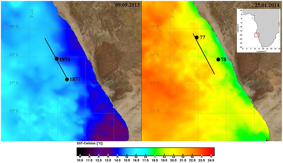
Figure 1. Map of the investigation area with sea surface temperature (SST) on 9 September 2013 and 25 January 2014 derived from GHRSST Level 4 data set (JPL MUR MEaSUREs Project, 2010). The positions of the stations for filling the tanks are indicated.

FIGURE 2

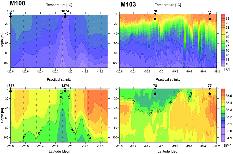
Figure 2. Vertical distribution of temperature (top) and salinity (bottom) at transects across an upwelled water body (filament) during the main upwelling season (left: M100, microstructure profiler data) and austral summer (right: M103, undulating CTD data). The bold black dots indicate the water sampling positions and depth. The positions of the transects are indicated in Figure 1.

During winter conditions, with low solar heating and strong wind forcing, the SST is a good indicator for the location of upwelling filaments and plumes of upwelled water. The in-situ distribution patterns of temperature and salinity coincide very well (left panels in Figure 2) and fit to the SST. The sampled upwelling filament is characterized by its cool and less saline core.

In austral summer the wind forcing is weaker and thus the amount of upwelled water is lower. The high heat flux due to strong solar radiation leads to fast warming of the surface layer. Therefore, in certain distance from the coast the upwelled water is not detectable by SST alone. The warm surface layer masks the upwelled water body in SST, but it is clearly indicated by its low salinity (right panels in Figure 2).

At the selected stations, 3 replicate tanks were filled with 90 L of upwelled water (“inside” the filament) or oceanic surface water (“outside” the filament) taken by means of large rosette water samplers (10 L per sampler) which were combined with a CTD SBE911+ and a log quantum scalar irradiance sensor (QSP-2350). For simulating the mixing, a set of three tanks was filled half with “inside” water and half with “outside” water. The tanks filled with the water from inside and outside the filament and the mixed water from the “winter” cruise M100 were marked with numbers IW, OW and MW, respectively, and those from the “summer” cruise M103 correspondingly with IS, OS, and MS. The water originated from 5 m depth on cruise M100 and from 10 m depth on cruise M103 (Figure 2). Some more details on the sampling stations and the starting conditions of the tanks are given in Table 1.

TABLE 1

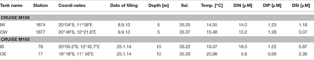
Table 1. Characteristics of the upwelling water (called “inside”, tanks marked with “I”) and oceanic water (called “outside” the filaments, tanks marked with “O”) for filling the tanks.

The mesocosms were nearly-cylindrical, white polyethylene barrels with a wide opening covered by a lid. The light transmittance of the barrel material was determined by measuring the light intensity inside and outside the tanks, with and without the lid, using the spherical sensor of the LI-COR data logger LI-1000. The photosynthetic active radiation (PAR) was reduced by the wall and lid of the tank to 50% of the external PAR. The tanks were placed on deck such that unequal shading was prevented and all tanks received nearly the same amount of light. As cloudy conditions prevailed during cruise M100, the water in the tanks stayed in the natural temperature range from 12.1 to 19.0°C and it was not necessary to prevent warming. During cruise M103, sunny weather prevailed and prompted us to span a screen over the tanks, which reduced the light intensity at bright sunshine e.g., from 1700 to 310 μE m⁻² s⁻¹ (i.e., to 18%) and changed the spectrum to green color, which nearly represented the light quantity and quality at 10 m depth.

All tanks were manually stirred three times a day (morning, noon, evening) by means of a carefully cleaned polyvinylchloride-paddle. At the same time, temperature was controlled. After the stirring in the morning, samples were taken by means of a big plastic beaker, which was carefully rinsed after each dipping. At least 3 L of sample were needed from each tank every sampling day. In order to avoid quick emptying of the tanks, we took samples after filling the tanks every third day from 11 September (= day 3) to 26 September 2013 (= day 18) during cruise M100. As it turned out from first analyses that processes proceeded quicker than expected, we changed the sampling frequency to 2 days from 25 January (= day 0) to 06 February 2014 (= day 12) on cruise M103.

Dissolved Inorganic Nutrients

The nutrient samples were filtered through disposable syringe filters (0.45 μm) immediately after sampling, filled in pre-rinsed 50 ml polyethylene bottles, frozen upright (−20°C), and analyzed in the shore-based laboratory after the expedition. Dissolved inorganic nitrogen (DIN), i.e., nitrate (${\text{NO}}_3^{-}$), nitrite (${\text{NO}}_2^{-}$), and ammonium (${\text{NH}}_4^{+}$), as well as phosphate (DIP) and silicate (DSi) were measured by a continuous flow injection system (Skalar SAN plus System) according to methods described by Grasshoff et al. (1999).

Particulate Organic Matter

From the nutrients in particulate matter only the particulate nitrogen (PN) was analyzed, together with the particulate carbon (PC). They can roughly be considered as particulate organic nitrogen and particulate organic carbon because inorganic particulate fractions are not relevant. Depending on the contents of particulate matter, 125–500 ml water were filtered through a pre-combusted Whatman GF/F filter of 2.5 cm diameter. The filters were dried at 60°C and stored under dry conditions until analysis. The PN and PC retained on the filters were measured using a continuous-flow isotope ratio mass spectrometer (THERMO Finnigan, Delta V).

Optical Properties

Optical measurements were performed in the tank experiment of cruise M103, but not on cruise M100. They allowed to follow the development of the spectral absorption of particulate matter (ap) and of colored dissolved organic matter (ay = CDOM, yellow substances).

Seawater was filtered under low vacuum through Whatman GF/F glass fiber filters (pore size approximately 0.7 μm). These filters were used to estimate the absorption of particulate material ap(λ) using the filter-pad method (Bricaud and Stramski, 1990). The absorption coefficients were measured using a dual-beam Perkin Elmer Lambda-35 spectrophotometer in the wavelength range of 400–750 nm with 1 nm intervals. Bricaud and Stramski (1990) introduced a method to divide the absorption coefficient of total particulate matter ap(λ) into the contribution of phytoplankton aph(λ) and detritus ad(λ). The phytoplankton absorption aph(440) represents the absorption at the chla maximum at 440 nm.

The filtered water was collected and measured in a 10 cm cuvette using the Perkin Elmer Lambda 35 instrument in the wavelength range between 300 and 750 nm with increments of 1 nm. Milli-Q water served as reference. The water was stored in a dark bottle to exhaust air bubbles in freshly produced water. The spectral absorption coefficients ay(λ) were calculated according to Kirk (1994) from the measured spectral absorbance and optical path length (length of the cuvette). The spectral dependence of CDOM absorption is characterized by an exponential increase to shorter wavelengths with a maximum in the ultraviolet spectral range (Jerlov, 1976; Kirk, 1994). The exponential slope was determined by fitting the curve in the spectral range between 350 and 550 nm (see also Neumann et al., 2015). The wavelengths of 380 and 440 nm served as references. The absorption coefficient at 380 nm is used for comparison in the experiments to describe the dissolved organic derivative products produced in the tanks.

Phytoplankton Pigments

Chlorophyll a (chla) served as a proxy for total phytoplankton biomass. Water samples (150–600 ml) were filtered onto Whatman GF/F filters, which were placed into Eppendorf vials and frozen in liquid nitrogen, afterwards extracted with 96% ethanol and measured with a TURNER fluorometer (10-AU-005).

The samples of the year 2013 were analyzed according to the method described by HELCOM (2014), with application of the recommendations by Wasmund et al. (2006), and the fluorometric measurement according to Welschmeyer (1994). This method is robust, but does not correct for the disturbing pheopigment a (pheoa) which is considered as degradation product of the chla. As pheoa may accumulate in the tanks, we used the acidification method of Lorenzen (1967) in addition to the above mentioned method in 2014.

Phytoplankton Biomass and Composition

The water samples (250 ml) for qualitative and quantitative phytoplankton analyses were preserved with 1 ml neutral Lugol solution. Subsamples (25 ml) were allowed to settle the particles according to the traditional method of Utermöhl (1958). Phytoplankton was counted and assigned to taxa and size classes in an inverted microscope (NIKON). The biomass was calculated according to stereometric formulas as prescribed in the manual of HELCOM (2014). This biomass calculation overvalues the diatoms because it includes their large vacuole that is poor in organic substances. For comparisons with other parameters, carbon is a better-suited universal unit. Therefore, we derived carbon from the biomass data using the formulas of Menden-Deuer and Lessard (2000).

Zooplankton Abundance and Composition

Specific microzooplankton analyses were performed only during the summer experiment (cruise M103). Because of the high effort for analyses, sampling was done only every 4th day and only from one (but always the same) of the triplicate tanks. For the determination of the composition and abundance of the main microzooplankton groups (50–200 μm), 5 L of water from each barrel has been filtered using a sieve with a mesh size of 50 μm. The samples were preserved in a 4% formaldehyde-seawater solution buffered with sodium-tetraborate for later analyses. In the home laboratory, samples were transferred into a sorting fluid composed of 94.5% fresh water, 5.0% propylene glycol, and 0.5% propylene phenoxetol according to Steedman (1976). The microzooplankton was identified to the species level or to the nearest taxonomic level that was possible owing to the morphological characteristics using a stereomicroscope. It was counted for each taxon and the abundance was expressed as individuals m⁻³. The data of microzooplankton abundance was not converted to biomass data in our studies because conversion factors are rather uncertain or not available. The size class smaller than 50 μm was considered in the phytoplankton samples. Mesozooplankton (>200 μm) was not representatively contained in the rather small sample volume and therefore disregarded.

Production and Respiration

The rates of the community's growth and loss processes can be measured simultaneously by the light-and-dark-bottle oxygen method (Gaarder and Gran, 1927). These parameters comprise oxygen-producing (photosynthesis) and oxygen-consuming (respiration) processes of the community enclosed in the incubation bottles. The net community production is measured in the light bottle and the respiration in the dark bottle. The net community production includes respiration processes and can be negative if respiration exceeds photosynthesis.

The production and respiration rates were measured by the oxygen method with temperature-compensated optical oxygen sensors. From each tank, a glass bottle of 250 ml contents was completely filled with water, supplied with a magnetic stirrer and closed by a silicone stopper, avoiding any air bubbles. Each stopper had a bore to hold an optical oxygen sensor (IntelliCal, Hach-Lange Berlin). The 9 bottles were stirred by a magnetic stirring rod with 400 rpm under temperature-controlled conditions (12–14°C). The incubation temperature was slightly lower than the ambient temperature in order to increase oxygen solubility. As it was important to prevent the formation of oxygen bubbles owing to over-saturation, we applied the dark incubation for respiration measurements first and switched on the light after 5 h, using OSRAM “Biolux” which provided 50 μE m⁻² s⁻¹ in the middle of the bottles.

The principle is shown by an example (Figure 3). The oxygen concentrations decreased continuously in the dark, and increased after the light was switched on at time step 60. The oxygen changes in tanks OW1 to OW3 were insignificant. The three replicate tanks showed a good agreement.

FIGURE 3

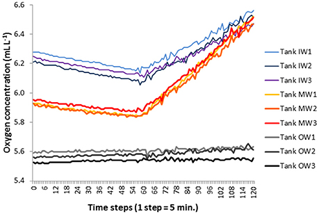
Figure 3. Example of the oxygen evolution in 5-h dark incubations followed by 5-h light incubation in the water taken from the tanks on 11.9.2013 (= day 3). The data from the three replicate tanks are shown separately.

Results

Hydrographic Conditions in the Tanks

As all 9 tanks of each experiment were exposed to similar global radiation, temperature did not differ significantly between the tanks. Therefore, we abstain from presenting the extensive temperature records. The starting conditions are given in Table 1. The temperature in the tanks (after stirring) fluctuated between 13.4 and 16.8°C during the experiment from late winter 2013 and between 19.1 and 24.2°C during the experiment from summer 2014.

The salinity increased slightly to the same extent in all tanks due to evaporation. Maximum increase occurred in summer, e.g., in the tanks IS from 35.22 to 35.39 and in the tanks OS from 35.33 to 35.51 during the investigation period.

Dissolved Inorganic Nutrients

Unexpectedly, the DIN and DIP concentrations at the stations sampled inside (IW) and outside of the filament (OW) during the M100 sampling campaign showed similar values (Table 1) and were reflected in comparable starting conditions (Figure 4A). During the M103 sampling campaign the water sampled inside the filament (IS) showed higher nutrient concentrations than the water sampled outside the filament (OS). The DIN was almost exclusively composed of nitrate during the first 2–3 days. Only in tanks OW, nitrate was high (10.6 μM) until day 6. Nitrite was insignificant all the time. Ammonium showed some peaks (Figures 4B, 5B), but with high differences between the tanks, leading to high standard deviations. The DSi concentrations in IW and OW tanks were very low (Table 1) indicating that silicon-dependent phytoplankton may be limited by silicon already at the start of the experiments.

FIGURE 4

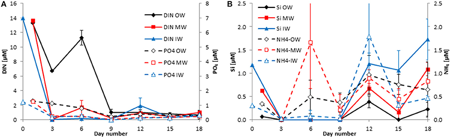
Figure 4. Development of the concentrations of DIN and DIP (A) as well as silicate and ammonium (B) in the tanks of the late winter experiment 2013 (cruise M100). Mean values and standard deviations of the three replicate tanks are shown.

FIGURE 5

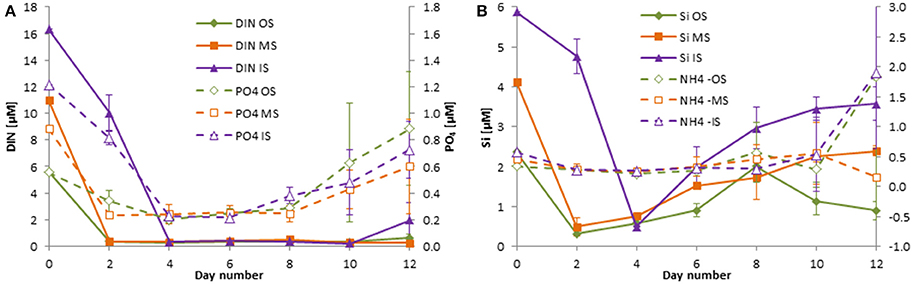
Figure 5. Development of the concentrations of DIN and DIP (A) as well as silicate and ammonium (B) in the tanks of the experiment from summer 2014 (cruise M103/2). Mean values and standard deviations of the three replicate tanks are shown.

The inorganic DIN:DSi:DIP molar ratios were 11.4: 0.96: 1 inside the filament and 10.4: 0.05: 1 outside the filament in winter 2013. They are calculated as 13.4: 4.8: 1 inside the filament and 10.1: 4.3: 1 outside the filament in summer 2014.

The standard deviations are in most cases small, indicating a good agreement between the replicate tanks. They are exceptionally high only on the last 2 days of the experiment from summer 2014 (Figure 5A) because DIN and DIP concentrations increased strongly by day 10 in one of the tanks IS and by day 12 in another tank of the IS-series. Such diverging developments at the end of mesocosm experiments are not unusual.

Particulate Organic Matter

The decrease in inorganic nutrients should lead to a respective increase in organically bound nutrients. Indeed, the exceptional DIN peak on day 6 in tanks OW and to a lesser degree in tanks MW was related to a stagnation in the PN increase (Figure 6A). Generally, the DIN consumption of about 14 μM in the winter experiment (Figure 4A) led to an increase in PN by 14 μM at least in tanks IW (Figure 6A). In the summer experiment, not the complete DIN consumption could be recovered in the particulate fraction (Figures 5A, 6B). It has to be admitted that the peaks in PN and PC are missed in the summer experiment because samples were taken only on days 0, 4, and 8.

FIGURE 6

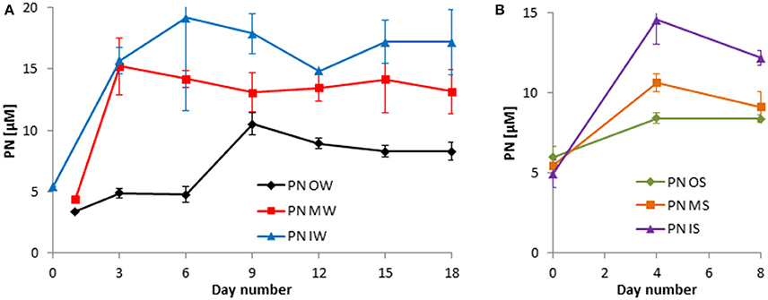
Figure 6. Development of the particulate nitrogen (PN) in the tanks of the experiment from winter 2013 (A) and summer 2014 (B). Mean values and standard deviations of the three replicate tanks are shown.

The development in PC concentrations is closely related to that of the PN concentrations (Figures 6, 7).

FIGURE 7

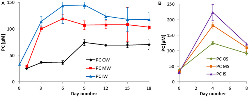
Figure 7. Development of the particulate carbon (PC) in the tanks of the experiment from winter 2013 (A) and summer 2014 (B). Mean values and standard deviations of the three replicate tanks are shown.

Optical Properties

Already the visual control revealed that the water in the tanks was very different depending on its origin. The water was turbid in tanks filled in the filament and very clear in tanks filled outside the filament on cruise M100 (winter 2013). In the experiment from summer 2014, the differences were smaller at the beginning, but tanks OS became clear after day 4, tanks MS after day 5, and tanks IS after day 7. As an objective tool for the documentation of these appearances, the optical properties were measured during the experiment from summer 2014. It proved that the replicates were very similar, reflected in the low standard deviations in Figure 8. The light absorption characteristics delivered information about the phytoplankton growth (Figure 8A) and the dissolved derivative metabolic products mostly produced by the decaying detritus (Figure 8B) in the tanks. The phytoplankton absorption was similar in the original water inside and outside the filament (day 0; mixed water not measured that day), as also found in the chla data (Figure 9B). After a gap in the data on day 2, a 7-fold increase was measured by day 4 in the water from inside the filament whereas the phytoplankton absorption in the water from outside the filament was only doubling and that in the mixed water ranged in between. These differences vanished by the end of the experiment.

FIGURE 8

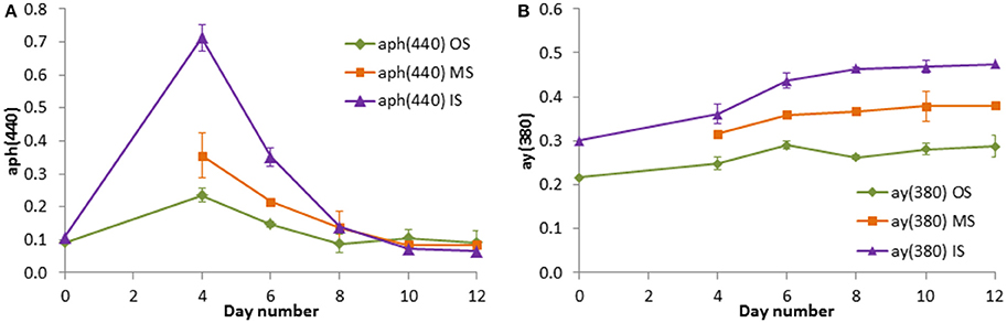
Figure 8. Light absorption coefficients by phytoplankton at 440 nm (A) and by CDOM at 380 nm (B) in the tank experiment on cruise M103. Mean values and standard deviations of the three replicate tanks are shown.

FIGURE 9

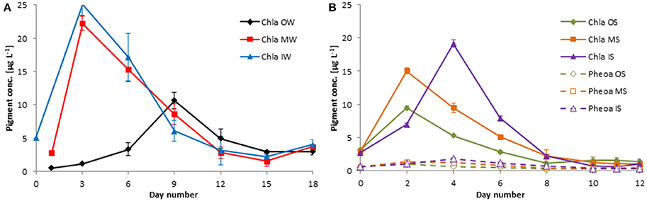
Figure 9. Development of the chla concentrations in winter 2013 (A) and of the chla and pheoa concentrations in summer 2014 (B). Mean values and standard deviations of the three replicate tanks are shown.

The absorption of yellow substances (CDOM) was rather different in the initial samples. In the “inside” (filament) water, the absorption was higher than in the “outside” water. The differences between the tanks became even larger during the experiment and the “mixed” water stayed just between the original waters. Obviously, the CDOM increased with the highest increase in the inside water between days 4 and 8 when the strongest decrease in the chla concentration and in the phytoplankton absorption was observed.

Chlorophyll

The chla concentrations revealed a much higher phytoplankton biomass inside the filament than outside at the beginning of the experiment in winter 2013 (Figure 9A). The chla concentrations in tanks “MW” had increased very quickly to its maximum value already 2 days after the start. Despite dilution with the “outside” water, chla concentrations in the “mixed” water reached almost the concentrations of the “inside” water. It means that phytoplankton growth was roughly two times higher in the “mixed” water than in the “inside” water. After the peak, chla concentrations declined steadily in the “mixed” and “inside” water. The chla concentrations in the water from outside the filament increased much slower, reached a smaller peak on day 9, and decreased afterwards.

The development in the chla data from the experiment of the summer 2014 (Figure 9B) is in very good agreement with the light absorption by phytoplankton (Figure 8A). The gap in the optical data from day 2 is closed by chla data. They show a much stronger phytoplankton growth in the mixed water that in the original water from inside and outside the filament by day 2. This is in agreement with the experiment from winter 2013, but in contrast to 2013, it was the “outside” water whose phytoplankton content decreased already after day 2 whereas the phytoplankton in the “inside” water continued growing.

Primary Production and Respiration

The oxygen method allowed measuring net community production (Figures 10A, 11A) and respiration (Figures 10B, 11B) in parallel. In the far most cases, net community production was positive; that means photosynthesis exceeded respiration and the system was autotrophic. The respiration (oxygen consumption) of the community is presented as positive values. Negative values, i.e., oxygen production in the dark as found until day 6 in tanks OW (Figure 10B), are considered as artifacts. They may occur if a presumed drift of the sensors is larger than the very small respiration rates. Details on these “negative” measurements are exemplified in Figure 3.

FIGURE 10

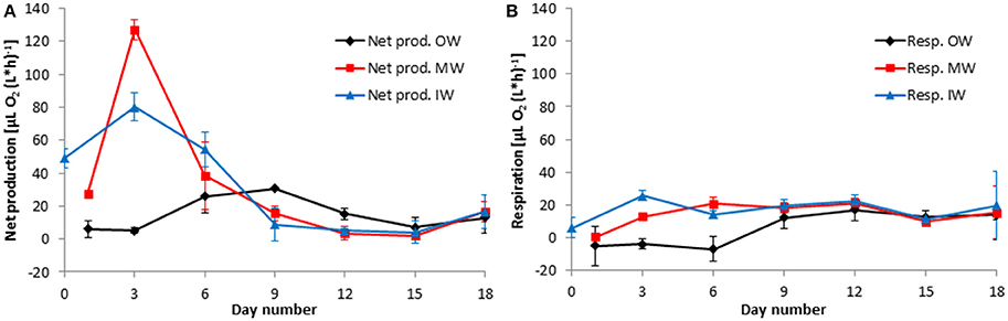
Figure 10. Development of the net community production (A) and respiration rates (B) in the tanks of the experiment from winter 2013. Mean values and standard deviations of the three replicate tanks are shown.

FIGURE 11

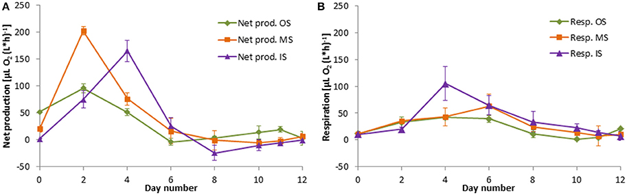
Figure 11. Development of the net community production (A) and respiration rates (B) in the tanks of the experiment from summer 2014. Mean values and standard deviations of the three replicate tanks are shown.

After mixing the original waters in the tanks “MW” and “MS,” net community production increased strongly and reached a peak within 2 days, both in the winter (Figure 10A) and in the summer (Figure 11A) experiment.

Phytoplankton

The species composition in the original waters from the winter experiment (Figure 12A) was highly different. The filament water (“IW”) was dominated by Corethron hystrix, small unidentified Gymnodiniales and other flagellates (Teleaulax, Pyramimonas) whereas the water from outside the filament (“OW”) was dominated by Gymnodiniales and Coccosphaerales. After filling the filament water into the tanks (“IW” and “MW”), phytoplankton biomass increased extremely within 3 days, mainly by the growth of C. hystrix. It has to be considered, that tanks “MW” were filled with only half of the concentration of tanks “IW” because the mixed water was diluted with the poor water from outside the filament. If the Corethron concentration in tanks “MW” is multiplied by two, it turns out that growth was even slightly higher in tanks “MW” than in tanks “IW.” The similarity in trends and species composition in tanks “IW” and “MW” revealed that the influence of the filament water was overwhelming in the mixed water, whereas the phytoplankton from outside the filament could not grow in the mixed water. The phytoplankton growth and composition was completely different in the tanks “OW.” The biomass maximum was only reached on day 9 by growth of small unidentified pennate diatoms (Pennales, 15 μm), and a few centric diatoms (Centrales like Rhizosolenia spp. and Proboscia spp.). The diatoms decreased after day 9, followed by dinoflagellates (e.g., Prorocentrum minimum) and other flagellates. Perhaps some of the unidentified flagellates were Coccosphaerales that lost their coccoliths since many single coccoliths were found in some samples. According to Siegel et al. (2007) and Siegel et al. (2014), light-resistant coccolithophores may develop in the frontal area between the upwelled and oceanic water in persistent shallow surface filaments.

FIGURE 12

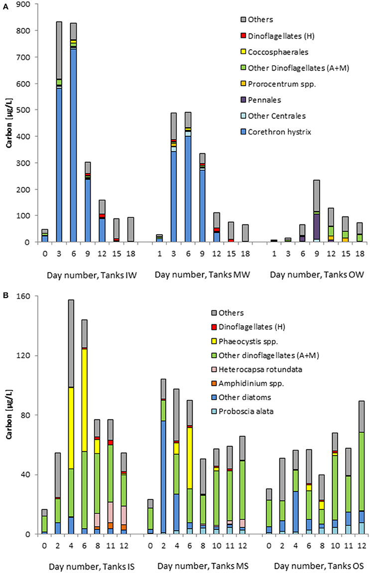
Figure 12. Development of the biomass (wet weight) of the most important phytoplankton taxa in the tanks containing water from “inside” (IS) and “outside” (OS) the filament and mixed water (MS), on cruise M100 (A) and on cruise M103 (B). Dinoflagellates are split into an autotrophic+mixotrophic (A+M) and a heterotrophic (H) group. Mean values of the three replicate tanks are shown.

The phytoplankton of the summer experiment, as far as identifiable, was completely different from that of the winter experiment (Figure 12B). The original water from inside the filament contained unidentified Gymnodiniales, Peridiniales and Centrales as well as Cylindrotheca closterium, dinoflagellates of the Diplopsalis-complex, and the heterotrophic Protoperidinium spp. The original water from outside the filament contained a lot of unidentified Gymnodiniales and Centrales as well as lower biomass of identified species like Proboscia alata, Lioloma elongatum, C. closterium, Gyrodinium spirale, Planktoniella sol, Rhizosolenia spp., Protoperidinium spp., and Scrippsiella spp. The differences between the two water bodies were not as large as in the winter experiment. In contrast to the winter experiment, the mixing of these waters (tanks “MS”) resulted in a clearly faster growth than in the original waters within 2 days, realized mainly by small unidentified Centrales (3–7 μm). Components of the two original waters grew in the mixed water: P. alata, L. elongatum, and P. sol which originated from outside the filament as well as Phaeocystis sp., Heterocapsa rotundata, and Amphidinium sp. from the filament water.

Microzooplankton

As many of the heterotrophic dinoflagellates might pass the zooplankton sieve, they were routinely counted in the phytoplankton samples. Their biomass is shown in Figure 12 and turns out to be very low in comparison with the autotrophic biomass. In the winter experiment, they were the only heterotrophic group investigated. In the summer experiment, also the complete microzooplankton was analyzed by means of specific methods described in section Zooplankton abundance and composition (Figure 13). As the data are variable, the abundance in tank MS at the beginning of the experiment is not exactly the average of the two original waters. However, all zooplankton groups of the original waters are represented in the mixed water. Appendicularia originate from the filament water (IS). For the Tintinnidae, the opposite is the case: they are typical for the offshore waters and therefore grow well in tank OS but do even not survive in the mixed water (tank MS). Foraminifera were sparse at the beginning but grew in tanks IS and OS. The abundance of the copepods increased strongly in tank IS and in a later stage of our experiment also in tank OS. They were the most quickly growing group, but were also quickly declining after their peak.

FIGURE 13

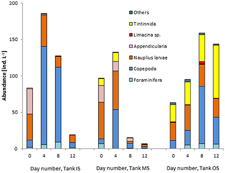
Figure 13. Development of the abundance of the microzooplankton groups in the tank containing water from “inside” (IS) and “outside” (IS) the filament and mixed water (MS) during the summer experiment on cruise M103.

Obviously, the microzooplankton could not take benefit of the rapidly blooming phytoplankton. It seems to be sensitive to suddenly changing conditions. On day 4, the total abundance in tank MS was still roughly the mean value of tanks IS and OS. By day 8, the total abundance in tank MS has drastically decreased. Foraminifera, Appendicularia, and Tintinnidae disappeared successively from tank MS.

Discussion

The Consistent Development of the Different Parameters

The two experiments were conducted in different seasons with different upwelling intensities. In the first experiment, carried through in late winter 2013, the growth of phytoplankton inside the filament was much faster than outside, where the peak was smaller and retarded. In the second experiment, carried through in summer 2014, the filaments were only poorly developed and the phytoplankton growth in the “inside” water was delayed in comparison with the “outside” water. However, in both experiments, the peaks of chla concentrations, net primary production, and phytoplankton biomass were clearly higher in the “inside” water in comparison with the “outside” water. Nevertheless, the mechanisms of the frontal mixing and biological reactions are the same under the different conditions. The progressions of the different parameters fit together to a consistent image that can be shortly summarized as follows.

The two experiments (winter and summer) started with relatively low phytoplankton biomass, which is also reflected in the chla concentrations and in summer 2014 in the light absorption by phytoplankton. Turbid stages of the water coincided with high light absorption [aph(440)] and chla concentrations. Obviously, the phytoplankton found optimal growth conditions in the tanks, causing a strong increase in net community production rates, which means that photosynthesis (phytoplankton gross production; not shown) was strongly exceeding the community respiration. The phytoplankton growth led to a quick nutrient decrease and exhaustion of the limiting nutrient within 2–4 days (exception in tanks OW: 9 days), followed by a decline in phytoplankton biomass. Phytoplankton growth and decline is obviously controlled by nutrient availability (bottom-up), but grazing by zooplankton (top-down) may also have an influence although a clear relationship between phytoplankton biomass and zooplankton abundance data could not be ascertained. Excretion and the degradation of particulate organic matter (mainly detritus) led to an enrichment of dissolved organic matter, indicated by the light absorption by CDOM at 380 nm.

Nutrient Ratios and Limitations of Phytoplankton Growth

Exploring the nutrient concentrations in the tanks supports our aim of tracing the plankton development in mixed waters in comparison with the original waters. The nitrate concentrations in the “inside” water at the beginning of the experiment indicates that this was not freshly upwelled water but it was on the border to maturing upwelled water if the definition for maturing upwelled water (nitrate concentrations varying between 2 and 15 μM) by Barlow (1982) is adopted. We have data from freshly upwelled surface water from cruise M100 (27 μM DIN, 17 μM Si, 1.7 μM DIP), which show that the nutrient concentrations had already strongly decreased up to the start of our experiment.

The inorganic DIN:DIP ratios at the beginning of the experiments were always lower than the canonical Redfield ratio of 16 (Redfield, 1958; Redfield et al., 1963), suggestive of a nitrogen deficit with respect to phosphorus. The DIN was depleted from day 3 in tanks IW and MW and from day 2 in tanks OS and MS, whereas DIP was still present in low concentrations indicating that nitrogen was limiting phytoplankton growth. At that time, net primary production and chla concentrations reached their maxima and declined afterwards because of severe nutrient limitation. In the “outside” water of the winter experiment (tanks OW), the nutrients decreased more slowly, dropping to a minimum only by day 9 when net primary production, chla concentration and phytoplankton biomass reached their maximum.

The low DIN:DIP ratios in the inorganic nutrients are already known from this area (Wasmund et al., 2005; Flohr et al., 2014). The limitation of phytoplankton growth by nitrogen is very common in marine waters (Ryther and Dunstan, 1971; Graziano et al., 1996; Hauss et al., 2012). Wasmund et al. (2015) assumed that nitrogen fixing cyanobacteria should benefit from the surplus phosphorus in the Benguela region. However, they could not find significant nitrogen fixation there. Also in our present study, nitrogen-fixing cyanobacteria did not occur. Therefore, nitrogen limitation seems to stay a long-lasting phenomenon in this upwelling region, as already concluded from earlier mesocosm experiments (Wasmund et al., 2014).

DIN uptake rates were high on the first 2–3 days of the experiment. They were calculated as 4.6, 6.8, and 3.3 μmol/(l*d) in tanks IW, MW, and OW, respectively, and as 3.2, 5.3, and 2.6 μmol/(l*d) in tanks IS, MS and OS, respectively. The highest DIN uptake rates were measured in the mixed water, which indicates that mixing of the two different waters creates new conditions, which are not the average of these two waters. Our DIN uptake rates are in the range measured by Benavides et al. (2014) using ¹⁵N-labeled substrates. They found new production rates of 17.8 and 3.9 mmol N/(m² h) in freshly upwelled and matured water, respectively, which are equivalent to 10.7 and 2.3 μmol/(l*d), respectively, in a 40 m deep water column in the northern Benguela region.

For diatoms, also silicate limitation has to be considered especially because DSi concentrations were very low (cf. Krause et al., 2015). The optimal DIN:DSi ratios for diatoms are variable (Brzezinski, 1985), but for rough estimates a molar ratio of DIN:DSi = 1.25 is applicable (Sarthou et al., 2005). The DIN:DSi ratios in all tanks at the beginning of the experiments were clearly higher, which indicates silicate limitation for diatom growth. Nevertheless, a strong diatom growth occurred, especially in tanks IW and MW. Obviously, the silicate requirement of C. hystrix is far less than expected. Harrison et al. (1977) found an increased average cellular DIN:DSi ratio of 5.1 for Si-starved or limited diatoms. Egge and Aksnes (1992) reported on diatom dominance if DSi concentration exceeded a threshold of approximately 2 μM. We question such general threshold as we found diatom growth at much lower DSi concentrations.

For example, the diatoms grew further by day 6 in tanks IW and MW despite lacking DSi in the water, but were obviously already starving as indicated by the decreasing chla concentrations and net primary production rates. Also the phytoplankton growth by day 9 in tanks OW was mainly caused by diatoms (Pennales) in spite of “zero” DSi. The tendency of increasing ammonium concentrations, with exceptional peaks in some tanks, is an indication of remineralization. It may also lead to a release of DSi, which might be ingested by the growing diatoms immediately. This uptake ceased with the decline of the diatom bloom, and DSi reappeared. Quick remineralization was found by Wasmund et al. (2014) already in an earlier tank experiment in this region.

In the experiment from summer 2014, diatom growth was relatively low in comparison with flagellates that are independent of DSi. Only directly after mixing the two different waters, diatoms grew suddenly (tanks MS, day 2), but decreased quickly due to nutrient (nitrogen and/or silicon) limitation.

The extremely low DSi concentrations are usual for the late successional state found in the mature offshore water (Hansen et al., 2014; Wasmund et al., 2014). The diatom growth on the basis of low or undetectable external DSi concentrations was astonishing on the first view but intelligible if considering that diatoms may continue growing for some generations with silicate limitation in chemostat cultures (Harrison et al., 1977).

Phytoplankton Biomass, Composition and Growth Rates

The phytoplankton biomass can be determined on a rather direct way by microscopy or via the chla concentration. For information on the total phytoplankton biomass, the more precise chla data are frequently preferred. Pitcher et al. (1993) measured chla concentrations of 0.01–0.31 μg/L in freshly upwelled southern Benguela water and maximum chla concentrations from 10.9 to 35.1 μg/L 9–13 days after the start of their microcosm experiments. In our experiments, the chla peaks were reached much earlier because the filament water was already maturing at the date of the start of the experiments, as also indicated by the relatively high starting concentrations in tanks IW and IS. Hansen et al. (2014) measured chla concentrations of 0.9–1.8 μg/L in rather freshly upwelled water in the northern Namibian coastal region. An extensive long-term study on chla concentrations in front of Walvis Bay is published by Louw et al. (2016).

The taxonomical composition of the nano- and microphytoplankton can be analyzed in routine work only by microscopy. Picoplankton was excluded from our microscopic analyses. It may contribute substantially to the phytoplankton biomass outside the front (Taylor et al., 2012), but is of minor importance in diatom-dominated waters (Walker and Peterson, 1991). We did not go into detail with the species composition but concentrated on the main phytoplankton groups. Already Pitcher et al. (1991) stated that phytoplankton communities changed in an unpredictable manner at the species level, but showed systematic trends on higher taxonomic levels.

The strong growth of diatoms in tanks IW and MW despite relatively low DIN and DSi concentrations was surprising. For example, the low starting biomass in tanks IW of 48 μgC/L corresponds to 4 μM C (Figure 12A). The PC measured in the same sample is, however, much higher (33.7 μM, Figure 7A). We think that the microscopically determined phytoplankton biomass on day 0 in tanks IW and MW is an underestimate. The PC values, despite not only including the phytoplankton, and chla concentrations are more realistic than phytoplankton counting results in this case. If we base our growth rate calculation on chla, the growth rate during the strongest increase in our experiments (tank MW from day 1 to day 3; Figure 9A) is 1.035 d⁻¹, which is clearly higher than that in the original filament water, accounting for 0.532 d⁻¹ in tank IW from day 0 to day 3. Pitcher et al. (1993) measured maximum specific growth rates from 0.57 to 1.96 d⁻¹ based on chla in experiments in freshly upwelled Benguela water.

It is known that diatoms have higher specific growth rates than dinoflagellates (Gallegos, 1992). Therefore, diatoms appear earlier than dinoflagellates in upwelled water (Hansen et al., 2014). According to Pitcher et al. (1998), diatoms are associated with upwelling water and dinoflagellates with the upwelling front. In general, diatoms are related to geostrophic or oceanic fronts and flagellates to the adjacent waters (Claustre et al., 1994; Allen et al., 2005; Taylor et al., 2012). In our experiment from winter 2013, the freshly upwelled water and the simulated frontal water (tanks IW and MW) were clearly dominated by diatoms. The weak filament from summer 2014 was dominated by dinoflagellates. However, also in this experiment, the mixing of “inside” and “outside” water led to a clear diatom growth. As some dinoflagellates may perform vertical migrations in order to utilize nutrients from deeper layers (Pitcher et al., 1998), their development may be reduced in the tanks as their migration is hampered.

Indeed, we found evidence of diurnal migration also in our tanks both in the winter and in the summer experiment. Greenish accumulations appeared near the water surface and in contact to the walls of the tanks around noon, extended toward the bottom by the evening and disappeared afterwards. The causative organisms were small green flagellates, which could not further be identified. Stratification, as prevailing in our tanks, might stimulate flagellates (Estrada and Berdalet, 1997; Pitcher and Nelson, 2006), but obviously, the three stirrings per day caused enough turbulence to create nearly natural conditions that are favorable for diatoms.

Zooplankton Abundance and Composition

After merging the two different waters, all zooplankton groups of the original waters were present for a while, but they could not benefit from this new condition and decreased strongly by day 8 in tank MS. The slight decline in phytoplankton biomass cannot be the main reason for the zooplankton collapse because a similar food concentration was sufficient in tank OS. Perhaps the phytoplankton composition was not appropriate as food. Walker and Peterson (1991) supported the hypothesis that growth rates of copepods depend not only on chla concentrations but on particle size too. They found dominance of small copepods in waters, where small phytoplankton cells dominated and large zooplankton in diatom-dominated water in the southern Benguela upwelling system. Probably, the sudden change in conditions is adverse for sensitive microzooplankton. Slower and gradual mixing in natural fronts may allow a better adaptation over a longer period. Ohman et al. (2012) found locally elevated zooplankton abundance and production of particle-grazing microzooplankton, including calanoid copepods and Appendicularia, in the California Current frontal system.

There is only little information about microzooplankton biomass in the northern Benguela Upwelling System. Irigoien et al. (2005) detected nano- and microzooplankton biomass between 200 and 800 mg C m⁻³ near the shore and less than 100 mg C m⁻³ in the offshore waters. However, the average zooplankton biomass in the northern Benguela system amounts to 1.3 g C m⁻² (Martin et al., 2015). The copepod biomass in maturing water of the southern Benguela upwelling area ranged from 11 to 86 mg C m⁻³, which accounted for 5 to 28% of the phytoplankton biomass, and its percentage increased with further aging of the water (Painting et al., 1993). Robinson et al. (2002) found a mean ratio of heterotrophic to autotrophic biomass of 0.8 in the northern Benguela upwelling region.

Production and Respiration

The community net production rates indicate the degree of autotrophy versus heterotrophy or growth versus loss processes in an ecosystem. The net production values were in almost all cases, primarily on the first few days of the experiment, positive. This results in an increase in total organic carbon. The phytoplankton biomass decreased, however, rather early. It was probably degraded to detritus. The clear phytoplankton biomass decline after day 6 in tanks IS and MS was not related to the zooplankton abundance. Grazing was probably not the controlling factor for the phytoplankton. However, Painting et al. (1993) think that grazing may have contributed significantly to the decline of the bloom during a drogue study in the southern Benguela upwelling plume, with copepods ingesting 5–10% of phytoplankton biomass in maturing upwelled water and, according to the literature, grazing is strongly increasing with the maturation of the water. They found an inverse relationship between copepod biomass and phytoplankton biomass.

In our tanks IS, the maxima of phytoplankton and zooplankton appeared at the same time (day 4), just when the respiration rate had its peak too. However, in most cases the respiration rate was not related to the zooplankton abundance probably because the zooplankton contributes only a small part to the community respiration. The respiration rates stayed relatively low until the end of the experiments. Obviously the detritus was not quickly decomposed by bacteria. Phytoplankton was widely unused and settled as detritus to the bottom of the tanks in the course of our experiments. However, the concentration of dissolved organic carbon has increased as indicated by CDOM (Figure 8B).

Various production and respiration data from upwelling areas are available in the literature, partly compiled by Robinson et al. (2002). Large-scale estimates of primary production in the northern Benguela region considering the different water bodies were made in special field studies by Wasmund et al. (2005). Hansen et al. (2014) measured primary production rates of 3.2 mg C m⁻³ h⁻¹ in freshly upwelled water, 5.6 mg C m⁻³ h⁻¹ during the diatom bloom in matured water and 2.2 mg C m⁻³ h⁻¹ in aged water on a transect in the northern Benguela region.

Painting et al. (1993) estimated that <10% of the primary production is consumed by mesozooplankton, a value supported by data of Moloney et al. (1991) in which <13% of the photosynthetically fixed carbon was estimated to be available to pelagic fish whereas 75% of the fixed carbon was lost through respiration and sinking. It is arguable to extrapolate our primary production and respiration data from short-term bottle incubations to larger spatial and three-dimensional units. We abstain from such extrapolations because our tank experiments were designed only for a mesoscale and short-term evaluation of the effect of a horizontal mixing across fronts.

The Effect of Mixing Different Water Bodies

Our primary aim was to study the effects of joining neighboring waters from both sides of a front. Physical transport processes had to be excluded in order to concentrate on the inherent biological processes. We showed clearly that the mixing of these different waters leads to higher growth in chla concentrations, net primary production, and phytoplankton biomass in comparison with the original waters. For interpretation of the figures it has to be remembered that the start conditions in the mixed water tanks was the average of the two original waters and therefore lower than the water from inside the filament. Therefore the growth rates in the mixed water tanks had to be higher than in the filament water tanks for reaching the same biomass. The strong growth in the mixed water proves that the biomass maximum described from fronts results not only from passive physical accumulation but mainly from local production, as already suggested by Claustre et al. (1994).

We discovered that the first phytoplankton growth pulse after frontal mixing is primarily based on intrinsic processes without external forcing. As the immense growth consumes the nutrient resources very quickly, primary production decreased already after 2–3 days in the tanks whereas the biomass decreased with a slight delay. Zooplankton growth could not follow with the same intensity and decreased strongly with the decrease in phytoplankton biomass. The phytoplankton biomass level became similar in tanks IS, MS and OS after day 8 and was obviously sufficient to feed the microzooplankton in tank OS. The strong decline in zooplankton abundance in tank MS could be caused by changes in phytoplankton composition e.g., decrease of diatom biomass and relative increase in dinoflagellate biomass. The chemical composition of some dinoflagellates may cause reduced grazing and avoidance behavior (Turner, 1997). A comparison of the data shown in Figures 12B, 13 does not suggest a top-down regulation of phytoplankton by zooplankton. The effect of grazing is low.

After the first pulse of intrinsic growth in the mixing zone, additional nutrients have to be delivered from deeper water layers to prolong the pre-existing bloom in the field (e.g., Allen et al., 2005; Li et al., 2012). Mesoscale eddies may displace the seasonal thermocline upwards and therefore introduce nutrients to the euphotic zone (Bibby and Moore, 2011). Winds inducing upwelling may erode subsurface phytoplankton patches, causing enhanced cross-frontal mixing leading to phytoplankton growth in the surface water of the front (Franks and Walstad, 1997). Allen et al. (2005) calculated a DSi supply rate from deeper water layers in an upwelling front in the northeast Atlantic of 0.34 mmol m⁻³ d⁻¹. Traganza et al. (1987) estimated wind-driven entrainment of nutrients from deeper layers into the mixed layer adjacent to the upwelling front at rates up to 0.76 μM nitrate d⁻¹ in the California coastal zone. In the southern Benguela system, Pitcher et al. (1998) found an upwards transport from the depth of the thermocline to the surface in the region of the upwelling front, where a surface bloom could grow and primary production rates were highest. Comparisons between tank experiments and parallel field observations of Wasmund et al. (2014) and Nausch and Nausch (2014) revealed that additional nutrients were supplied to the surface layer in the northern Benguela region. Moreover, actively migrating plankton organisms may contribute additional nutrients. Pitcher et al. (1998) observed vertically migrating dinoflagellates, which were descending during the night into nutrient-rich water layers. A migration to deeper water layers was blocked in our tanks and also further nutrient delivery by frontal upwelling was prevented. Therefore, nutrients were much quicker exhausted in the tanks than in the field.

Our tank experiments showed that phytoplankton may adapt quickly to new conditions if it is forced into strange water bodies. In contrast to zooplankton, it is not inhibited but even stimulated in these ecotones during the first few days. This proves true both in the high-upwelling late-winter season and in der low-upwelling summer season.

Conclusions

Studies undertaken in frontal areas detected enhanced phytoplankton production and biomass and explained this phenomenon by physical forcing. Intrinsic factors, i.e., the sole effect of merging the neighboring water bodies in frontal zones, could not be studied in the field up to now. In order to investigate the sole effect of mixing on the organisms living in these different waters, external forcing, e.g., nutrient input by frontal upwelling or invading organisms had to be excluded. This was realized by a mesocosm (tank) approach. The artificial mixing of different waters led to a sudden strong phytoplankton growth. It answered the question whether organisms benefit from new conditions if one water mass contained a resource in excess that limited the growth in the other water mass. The biomass boost lasted only a few days until depletion of the nutrients.

Field studies in frontal zones, reported in the literature, showed a much longer continuing biomass maximum at these boundary zones. The comparison of the field studies with our mesocosm studies revealed that continuous nutrient delivery is a main driver for these biomass maxima. Our approach excluded external forcing by purpose in order to study the short-term effects of simple joining of different plankton communities together with their natural environs. It was not designed to simulate long-term processes in fronts. Therefore, it did not allow calculations on nutrient budgets or transports. This may be possible by modeling, which was, however, beyond our scope.

Author Contributions

NW developed the approach, took part in cruises M100 and M103, conducted the tank experiments, measured primary production, and respiration, was responsible for the phytoplankton, chlorophyll and POC/PON sampling, and prepared the manuscript with contributions from all co-authors. HS took part in cruise M103, conducted the measurements on optical properties and processed satellite images. KB took part in cruises M100 and M103, did the zooplankton analyses and evaluations. AF took part in cruises M100 and M103, conducted the nutrient analyses. AH did the phytoplankton and chla analyses. VM took part in cruises M100 and M103, was cruise leader of M103 and sub-project leader in GENUS II, and conducted the hydrographical measurements.

Conflict of Interest Statement

The authors declare that the research was conducted in the absence of any commercial or financial relationships that could be construed as a potential conflict of interest.

Acknowledgments

The research was conducted within the framework of the project “Geochemistry and Ecology of the Namibian Upwelling System” (GENUS II; grant number 03F0650C), funded by the German Federal Ministry for Education and Research (BMBF). We are grateful to the leader of the project GENUS, Prof. Dr. Kay Emeis and its coordinator, Dr. Niko Lahajnar. Moreover, we appreciate the stimulating cooperation with the cruise leaders (Prof. Dr. Buchholz, VM). We thank Iris Liskow for the PC and PN measurements, Matthias Birkicht for the nutrient measurements, Regina Hansen for the phytoplankton analyses of cruise M100, Monika Gerth for the SST maps, and Dr. Juliane Brust-Möbius for supporting optical measurements during the cruise M103. The experiments on board the vessel were attended by Arnold De Klerk (Ministry of Fisheries and Marine Resources, National Research Institute Swakopmund, Namibia; on cruise M100) and Dr. Chibo Chikwililwa (Ministry of Fisheries and Marine Resources, National Marine Information and Research Centre Swakopmund, Namibia; on cruise M103). The Group of High Resolution Sea Surface Temperature (GHRSST) Multi-scale Ultra-high Resolution (MUR) SST data were obtained from the NASA EOSDIS Physical Oceanography Distributed Active Archive Center (PO.DAAC) at the Jet Propulsion Laboratory, Pasadena, CA (http://dx.doi.org/10.5067/GHGMR-4FJ01).

References

Allen, J. T., Brown, L., Sanders, R., Moore, C. M., Mustard, A., Fielding, S., et al. (2005). Diatom carbon export enhanced by silicate upwelling in the northeast Atlantic. Nature 437, 728–732. doi: 10.1038/nature03948

PubMed Abstract | CrossRef Full Text | Google Scholar

Barlow, R. G. (1982). Phytoplankton ecology in the Southern Benguela Curent. I. Biochemical composition. J. Exp. Mar. Biol. Ecol. 63, 209–228. doi: 10.1016/0022-0981(82)90179-4

CrossRef Full Text | Google Scholar

Benavides, M., Santana-Falcón, Y., Wasmund, N., and Arístegui, J. (2014). Microbial uptake and regeneration of inorganic nitrogen off the coastal Namibian upwelling system. J. Mar. Syst. 140(Pt B), 123–129. doi: 10.1016/j.jmarsys.2014.05.002

CrossRef Full Text | Google Scholar

Bibby, T. S., and Moore, C. M. (2011). Silicate:nitrate ratios of upwelled waters control the phytoplankton community sustained by mesoscale eddies in sub-tropical North Atlantic and Pacific. Biogeosciences 8, 657–666. doi: 10.5194/bg-8-657-2011

CrossRef Full Text | Google Scholar

Bricaud, A., and Stramski, D. (1990). Spectral absorption coefficients of living phytoplankton and nonalgal biogenous matter: a comparison between the Peru upwelling area and the Sargasso Sea. Limnol. Oceanogr. 35, 562–582. doi: 10.4319/lo.1990.35.3.0562

CrossRef Full Text | Google Scholar

Brown, P. C. (1984). Primary production at two contrasting nearshore sites in the southern Benguela upwelling region. 1977-1979. S. Afr. J. Mar. Sci. 2, 205–215. doi: 10.2989/02577618409504369

CrossRef Full Text | Google Scholar

Brown, P. C., and Hutchings, L. (1987). The development and decline of phytoplankton blooms in the southern Benguela upwelling system. 1. Drogue movements, hydrography and bloom development. S. Afr. J. Mar. Sci. 5, 357–391. doi: 10.2989/025776187784522801

CrossRef Full Text | Google Scholar

Brzezinski, M. A. (1985). The Si:C:N ratio of marine diatoms: interspecific variability and the effect of some environmental variables. J. Phycol. 21, 347–357. doi: 10.1111/j.0022-3646.1985.00347.x

CrossRef Full Text | Google Scholar

Buchholz, F. (2014). Physics, Biogeochemistry and Ecology of Upwelling Filaments and Boundary Zones Off Namibia - GENUS II - Cruise No. M100/1 - September 1 to October 1, 2013 - Walvis Bay (Namibia) to Walvis Bay (Namibia). DFG-Senatskommission für Ozeanographie. doi: 10.2312/cr_m100_1

CrossRef Full Text

Carr, M.-E., and Kearns, E. J. (2003). Production regimes in four eastern boundary current systems. Deep Sea Res. Part II 50, 3199–3221. doi: 10.1016/j.dsr2.2003.07.015

CrossRef Full Text | Google Scholar

Claustre, H., Kerhervé, P., Marty, J. C., Prieur, L., Videau, C., and Hecq, J.-H. (1994). Phytoplankton dynamics associated with a geostrophic front: ecological and biogeochemical implications. J. Mar. Res. 52, 711–742. doi: 10.1357/0022240943077000

CrossRef Full Text | Google Scholar

Duncombe Rae, C. M. (2005). A demonstration of the hydrographic partition of the Benguela upwelling ecosystem at 26°40′S. Afr. J. Mar. Sci. 27, 617–628. doi: 10.2989/18142320509504122

CrossRef Full Text | Google Scholar

Egge, J. K., and Aksnes, D. L. (1992). Silicate as regulating nutrient in phytoplankton competition. Mar. Ecol. Prog. Ser. 83, 281–289. doi: 10.3354/meps083281

CrossRef Full Text | Google Scholar

Estrada, M., and Berdalet, E. (1997). Phytoplankton in a turbulent world. Sci. Mar. 61, 125–140.

Google Scholar

Flohr, A., van der Plas, A. K., Emeis, K.-C., Mohrholz, V., and Rixen, T. (2014). Spatio-temporal patterns of C: N : P ratios in the northern Benguela upwelling system. Biogeosciences 11, 885–897. doi: 10.5194/bg-11-885-2014

CrossRef Full Text | Google Scholar

Franks, P. J. S. (1992). Sink or swim: accumulation of biomass in fronts. Mar. Ecol. Prog. Ser. 82, 1–12. doi: 10.3354/meps082001

PubMed Abstract | CrossRef Full Text | Google Scholar

Franks, P. J. S., and Walstad, L. J. (1997). Phytoplankton patches at fronts: a model of formation and response to wind events. J. Mar. Res. 55, 1–19. doi: 10.1357/0022240973224472

CrossRef Full Text | Google Scholar

Fréon, P., Barange, M., and Aristegui, J. (2009). Eastern boundary upwelling ecosystems: integrative and comparative approaches preface. Prog. Oceanogr. 83, 1–14. doi: 10.1016/j.pocean.2009.08.001

CrossRef Full Text

Gaarder, T., and Gran, H. H. (1927). Investigations of the production of plankton in the Oslo Fjord. Rapp. et Proc. Verb. Cons. Int. Explor. Mer. 42, 1–48.

Gallegos, C. L. (1992). Phytoplankton photosynthesis, productivity, and species composition in a eutrophic estuary: comparison of bloom and non-bloom assemblages. Mar. Ecol. Prog. Ser. 81, 257–267. doi: 10.3354/meps081257

CrossRef Full Text | Google Scholar

Grasshoff, K., Kremling, K., and Ehrhardt, M. (1999). Methods of Seawater Analysis. Weinheim: Wiley-VCH.

Google Scholar

Graziano, L. M., Geider, R. J., Li, W. K. W., and Olaizola, M. (1996). Nitrogen limitation of North Atlantic phytoplankton: analysis of physiological condition in nutrient enrichment experiments. Aquat. Microb. Ecol. 11, 53–64. doi: 10.3354/ame011053

CrossRef Full Text | Google Scholar

Hansen, A., Ohde, T., and Wasmund, N. (2014). Succession of micro- and nanoplankton groups in ageing upwelled waters off Namibia. J. Mar. Syst. 140(Pt B), 130–137. doi: 10.1016/j.jmarsys.2014.05.003

CrossRef Full Text | Google Scholar

Harrison, P. H., Conway, H., Holmes, W., and Davis, D. (1977). Marine diatoms grown in chemostats under silicate or ammonium limitation. III. Cellular chemical composition and morphology of Chaetoceros debilis, Skeletonema costatum, and Thalassiosira gravida. Mar. Biol. 43, 19–31. doi: 10.1007/BF00392568

CrossRef Full Text | Google Scholar

Hart, T. J., and Currie, R. I. (1960). The Benguela Current. Discov. Rep. 31, 123–297.

Hauss, H., Franz, J. M. S., and Sommer, U. (2012). Changes in N:P stoichiometry influence taxonomic composition and nutritional quality of phytoplankton in the Peruvian upwelling. J. Sea Res. 73, 74–85. doi: 10.1016/j.seares.2012.06.010

CrossRef Full Text | Google Scholar

HELCOM (2014). Manual for Marine Monitoring in the COMBINE Programme of HELCOM. – Internet, Updated January 2014. Available online at: http://www.helcom.fi/Documents/Action%20areas/Monitoring%20and%20assessment/Manuals%20and%20Guidelines/Manual%20for%20Marine%20Monitoring%20in%20the%20COMBINE%20Programme%20of%20HELCOM.pdf

Hutchings, L., van der Lingen, C. D., Shannon, L. J., Crawford, R. J. M., Verheye, H. M. S., Bartholomae, C. H., et al. (2009). The Benguela Current: an ecosystem of four components. Prog. Oceanogr. 83, 15–32. doi: 10.1016/j.pocean.2009.07.046

CrossRef Full Text | Google Scholar

Irigoien, X., Flynn, K. J., and Harris, R. P. (2005). Phytoplankton blooms: a ‘loophole’ in microzooplankton grazing impact? J. Plankton Res. 27, 313–321. doi: 10.1093/plankt/fbi011

CrossRef Full Text | Google Scholar

Jerlov, N. G. (1976). Marine Optics, Vol. 14. Amsterdam: Elsevier Oceanography Series.

JPL MUR MEaSUREs Project (2010). GHRSST Level 4 MUR Global Foundation Sea Surface Temperature Analysis. Ver. 2. PO.DAAC. Pasadena, CA. doi: 10.5067/GHGMR-4FJ01

CrossRef Full Text

Kirk, J. T. (1994). Estimation of the absorption and the scattering coefficients of natural waters by use of underwater irradiance measurements. Appl. Opt. 33, 3276–3278. doi: 10.1364/AO.33.003276

PubMed Abstract | CrossRef Full Text | Google Scholar

Krause, J. W., Brzezinski, M. A., Goericke, R., Landry, M. R., Ohman, M. D., Stukel, M. R., et al. (2015). Variability in diatom contributions to biomass, organic matter production and export across a frontal gradient in the California Current Ecosystem. J. Geophys. Res. Oceans 120, 1–16. doi: 10.1002/2014jc010472

CrossRef Full Text | Google Scholar

Lachkar, Z., and Gruber, N. (2012). A comparative study of biological production in eastern boundary upwelling systems using an artificial neural network. Biogeosciences 9, 293–308. doi: 10.5194/bg-9-293-2012

CrossRef Full Text | Google Scholar

Lahajnar, N., Mohrholz, V., Angenendt, S., Ankele, M., Annighöfer, M., Beier, S., et al. (2015). “Geochemistry and Ecology of the Namibian Upwelling System NAMUFIL: Namibian Upwelling Filament Study - Cruise No. M103 - December 27, 2013 to February 11, 2014 - Walvis Bay (Namibia) to Walvis Bay (Namibia). DFG-Senatskommission für Ozeanographie. doi: 10.2312/cr_m103

CrossRef Full Text

Landry, M. R., Ohman, M. D., Goericke, R., Stukel, M. R., Barbeau, K. A., Bundy, R., et al. (2012). Pelagic community responses to a deep-water front in the California Current Ecosystem: overview of the A-Front Study. J. Plankton Res. 34, 739–748. doi: 10.1093/plankt/fbs025

CrossRef Full Text | Google Scholar

Largier, J. L. (1993). Estuarine fronts - how important are they. Estuaries 16, 1–11. doi: 10.2307/1352760

CrossRef Full Text | Google Scholar

Lass, H.-U., and Mohrholz, V. (2008). On the interaction between the subtropical gyre and the subtropical cell on the shelf of the SE Atlantic. J. Mar. Syst. 74, 1–49. doi: 10.1016/j.jmarsys.2007.09.008

CrossRef Full Text | Google Scholar

Li, Q. P., Franks, P. J. S., Ohman, M. D., and Landry, M. R. (2012). Enhanced nitrate fluxes and biological processes at a frontal zone in the southern California current system. J. Plankton Res. 34, 790–801. doi: 10.1093/plankt/fbs006

CrossRef Full Text | Google Scholar

Lorenzen, C. J. (1967). Determination of chlorophyll and pheo-piments: spectrophotometric equations. Limnol. Oceanogr. 12, 343–346. doi: 10.4319/lo.1967.12.2.0343

CrossRef Full Text | Google Scholar

Louw, D. C., van der Plas, A., Mohrholz, V., Wasmund, N., Junker, T., and Eggert, A. (2016). Seasonal and inter-annual phytoplankton dynamics and forcing mechanisms in the northern Benguela upwelling system. J. Mar. Syst. 157, 124–134. doi: 10.1016/j.jmarsys.2016.01.009

CrossRef Full Text | Google Scholar

Lutjeharms, J. R. E., and Meeuwis, J. M. (1987). The extent and variability of South-East Atlantic upwelling. S. Afr. J. Mar. Sci. 5, 51–62. doi: 10.2989/025776187784522621

CrossRef Full Text | Google Scholar

Margalef, R. (1962). Succession in marine populations. Adv. Front. Plant Sci. 2, 137–188.

Google Scholar

Martin, B., Eggert, A., Koppelmann, R., Diekmann, R., Mohrholz, V., and Schmidt, M. (2015). Spatio-temporal variability of zooplankton biomass and environmental control in the northern Benguela upwelling system: field investigations and model simulation. Mar. Ecol. 36, 637–658. doi: 10.1111/maec.12173

CrossRef Full Text | Google Scholar

Menden-Deuer, S., and Lessard, E. J. (2000). Carbon to volume relationsships for dinoflagellates, diatoms and other protist plankton. Limnol. Oceanogr. 45, 569–579. doi: 10.4319/lo.2000.45.3.0569

CrossRef Full Text | Google Scholar

Mitchell-Innes, B. A., and Walker, D. R. (1991). Short-term variability during an anchor station study in the southern Benguela upwelling system: phytoplankton production and biomass in relation to species changes. Prog. Oceanogr. 28, 65–89. doi: 10.1016/0079-6611(91)90021-D

CrossRef Full Text | Google Scholar

Mohrholz, V., Eggert, A., Junker, T., Nausch, G., Ohde, T., and Schmidt, M. (2014). Cross shelf hydrographic and hydrochemical conditions and their short term variability at the northern Benguela during a normal upwelling season. J. Mar. Syst. 140(Pt B), 92–110. doi: 10.1016/j.jmarsys.2014.04.019

CrossRef Full Text | Google Scholar

Moloney, C. L., Field, J. G., and Lucas, M. I. (1991). The size-based dynamics of plankton food webs. II. Simulations of three contrasting southern Benguela food webs. J. Plankton Res. 13, 1039–1092. doi: 10.1093/plankt/13.5.1039

CrossRef Full Text | Google Scholar

Muller, A. A., Mohrholz, V., and Schmidt, M. (2013). The circulation dynamics associated with a northern Benguela upwelling filament during October 2010. Cont. Shelf Res. 63, 59–68. doi: 10.1016/j.csr.2013.04.037

CrossRef Full Text | Google Scholar

Nagai, T., Gruber, N., Frenzel, H., Lachkar, Z., McWilliams, J. C., and Plattner, G.-K. (2015). Dominant role of eddies and filaments in the offshore transport of carbon and nutrients in the California Current System. J. Geophys. Res. Oceans 120, 1–24. doi: 10.1002/2015JC010889

CrossRef Full Text | Google Scholar

Nausch, M., and Nausch, G. (2014). Phosphorus speciation and transformation along transects in the Benguela upwelling region. J. Mar. Syst. 140(Pt B), 111–122. doi: 10.1016/j.jmarsys.2014.04.020

CrossRef Full Text | Google Scholar

Neumann, T., Siegel, H., and Gerth, M. (2015). A new radiation model for Baltic Sea ecosystem modelling. J. Mar. Syst. 152, 83–91. doi: 10.1016/j.jmarsys.2015.08.001

CrossRef Full Text | Google Scholar

Ohman, M. D., Powell, J. R., Picheral, M., and Jensen, D. W. (2012). Mesozooplankton and particulate matter responses to a deep-water frontal system in the southern California Current System. J. Plankton Res. 34, 815–827. doi: 10.1093/plankt/fbs028

CrossRef Full Text | Google Scholar

Painting, S. J., Lucas, M. I., Peterson, W. T., Brown, P. C., Hutchings, L., and Mitchell-Innes, B. A. (1993). Dynamics of bacterioplankton, phytoplankton and mesozooplankton communities during the development of an upwelling plume in the southern Benguela. Mar. Ecol. Prog. Ser. 100, 35–53. doi: 10.3354/meps100035

CrossRef Full Text

Pitcher, G. C. (1988). Mesoscale heterogeneities of the phytoplankton distribution in St. Helena Bay, South Africa, following an upwelling event. S. Afr. J. Mar. Sci. 7, 9–23. doi: 10.2989/025776188784379170

CrossRef Full Text | Google Scholar

Pitcher, G. C., Bolton, J. J., Brown, P. C., and Hutchings, L. (1993). The development of phytoplankton blooms in upwelled waters of the southern Benguela upwelling system as determined by microcosm experiments. J. Exp. Mar. Biol. Ecol. 165, 171–189. doi: 10.1016/0022-0981(93)90104-V

CrossRef Full Text | Google Scholar

Pitcher, G. C., Boyd, A. J., Horstman, D. A., and Mitchell-Innes, B. A. (1998). Subsurface dinoflagellate populations, frontal blooms and the formation of red tide in the southern Benguela upwelling system. Mar. Ecol. Prog. Ser. 172, 253–264. doi: 10.3354/meps172253

CrossRef Full Text | Google Scholar

Pitcher, G. C., and Nelson, G. (2006). Characteristics of the surface boundary layer important to the development of red tide on the southern Namaqua shelf of the Benguela upwelling system. Limnol. Oceanogr. 51, 2660–2674. doi: 10.4319/lo.2006.51.6.2660

CrossRef Full Text | Google Scholar

Pitcher, G. C., Walker, D. R., Mitchell-Innes, B. A., and Moloney, C. L. (1991). Short-term variability during an anchor station study in the southern Benguela upwelling system: phytoplankton dynamics. Prog. Oceanogr. 28, 39–64. doi: 10.1016/0079-6611(91)90020-M

CrossRef Full Text | Google Scholar

Redfield, A. C. (1958). The biological control of chemical factors in the environment. Am. Sci. 46, 205–221.

Google Scholar

Redfield, A. C., Ketchum, B. H., and Richards, F. A. (1963). “The influence of organisms on the composition of seawater,” in The Sea, ed M. N. Hill (New York, NY: Wiley), 26–77.

Robinson, C., Serret, P., Tilstone, G., Teira, E., Zubkov, M. V., Rees, A. P., et al. (2002). Plankton respiration in the Eastern Atlantic Ocean. Deep Sea Res. Part I 49, 787–813. doi: 10.1016/S0967-0637(01)00083-8

CrossRef Full Text | Google Scholar

Ryther, J. H., and Dunstan, W. M. (1971). Nitrogen, phosphorus, and eutrophication in the coastal marine environment. Science 171, 1008–1013. doi: 10.1126/science.171.3975.1008

PubMed Abstract | CrossRef Full Text | Google Scholar

Sarthou, G., Timmermans, K. R., Blain, S., and Tréguer, P. (2005). Growth physiology and fate of diatoms in the ocean: a review. J. Sea Res. 53, 25–42. doi: 10.1016/j.seares.2004.01.007

CrossRef Full Text | Google Scholar

Shannon, L. V., and Nelson, G. (1996). “The Benguela: Large scale features and processes and system variability,” in The South Atlantic: Present and Past Circulation, eds G. Wefer, W. H. Berger, G. Siedler, and D. J. Webb (Berlin: Springer-Verlag), 163–210.

Siegel, H., Ohde, T., and Gerth, M. (2014). “The upwelling area off Namibia, the northern part of the Benguela current system,” in Remote Sensing of the African Seas, eds V. Barale and M. Gade (Dordrecht: Springer), 167–183.

Siegel, H., Ohde, T., Gerth, M., Lavik, G., and Leipe, T. (2007). Identification of coccolithophore blooms in the SE Atlantic Ocean off Namibia by satellites and in-situ methods. Cont. Shelf Res. 27, 258–274. doi: 10.1016/j.csr.2006.10.003

CrossRef Full Text | Google Scholar

Steedman, H. F. (1976). “General and applied data on formaldehyde fixation and preservation of marine zooplankton,” in Zooplankton Fixation and Preservation, ed H. F. Steedman (Paris: Unesco Press), 103–154.

Google Scholar

Stramma, L., and England, M. (1999). On the water masses and mean circulation of the South Atlantic Ocean. J. Geophys. Res. 104, 20863–20883. doi: 10.1029/1999JC900139

CrossRef Full Text | Google Scholar

Taylor, A. G., Goericke, R., Landry, M. R., Selph, K. E., Wick, D. A., and Roadman, M. J. (2012). Sharp gradients in phytoplankton community structure across a frontal zone in the California Current Ecosystem. J. Plankton Res. 34, 778–789. doi: 10.1093/plankt/fbs036

CrossRef Full Text | Google Scholar

Traganza, E. D., Redalje, D. G., and Garwood, R. W. (1987). Chemical flux, mixed layer entrainment and phytoplankton blooms at upwelling fronts in the California coastal zone. Cont. Shelf Res. 7, 89–105. doi: 10.1016/0278-4343(87)90066-5

CrossRef Full Text | Google Scholar

Turner, J. T. (1997). Toxic marine phytoplankton, zooplankton grazers, and pelagic food webs. Limnol. Oceanogr. 42, 1203–1214. doi: 10.4319/lo.1997.42.5_part_2.1203

CrossRef Full Text | Google Scholar

Utermöhl, H. (1958). Zur Vervollkommnung der quantitativen Phytoplankton-Methodik. Mitt. d. Internat. Vereinig. f. Limnologie 9, 1–38.

Walker, D. R., and Peterson, W. T. (1991). Relationships between hydrography, phytoplankton production, biomass, cell size and species composition, and copepod production in the southern Benguela upwelling system in April 1988. S. Afr. J. Mar. Sci. 11, 289–305. doi: 10.2989/025776191784287529

CrossRef Full Text | Google Scholar

Wasmund, N., Lass, H.-U., and Nausch, G. (2005). Distribution of nutrients, chlorophyll and phytoplankton primary production in relation to hydrographic structures bordering the Benguela-Angolan frontal region. Afr. J. Mar. Sci. 27, 177–190. doi: 10.2989/18142320509504077

CrossRef Full Text | Google Scholar

Wasmund, N., Nausch, G., and Hansen, A. (2014). Phytoplankton succession in an isolated upwelled Benguela water body in relation to different initial nutrient conditions. J. Mar. Syst. 140, 163–174. doi: 10.1016/j.jmarsys.2014.03.006

CrossRef Full Text | Google Scholar

Wasmund, N., Struck, U., Hansen, A., Flohr, A., Nausch, G., Grüttmüller, A., et al. (2015). Missing nitrogen fixation in the Benguela region. Deep Sea Res. 106, 30–41. doi: 10.1016/j.dsr.2015.10.007

CrossRef Full Text | Google Scholar

Wasmund, N., Topp, I., and Schories, D. (2006). Optimising the storage and extraction of chlorophyll samples. Oceanologia 48, 125–144. doi: 10.1016/j.drs.2015.10.007

CrossRef Full Text | Google Scholar

Welschmeyer, N. A. (1994). Fluorometric analysis of chlorophyll a in the presence of chlorophyll b and pheopigments. Limnol. Oceanogr. 39, 1985–1992. doi: 10.4319/lo.1994.39.8.1985

CrossRef Full Text | Google Scholar