Copepod Life Strategy and Population Viability in Response to Prey Timing and Temperature: Testing a New Model across Latitude, Time, and the Size Spectrum

1. Introduction

Calanoid copepods occupy a crucial position in marine food webs, the dominant mesozooplankton in many temperate and polar systems, important to packaging of microbial production in a form accessible to higher predators. They also represent the point at which biogeochemical processes, and numerical approaches like NPZ (nutrient–phytoplankton–zooplankton) models, start to be significantly modulated by life-history and behavioral constraints. The population- and community-level response of copepods to environmental change (temperature, prey availability, seasonality) thus forms a crucial filter lying between the biogeochemical impacts of climate change on primary production patterns and the food-web impacts that follow.

Across many scales in many systems, the response of fish, seabirds, and marine mammals to climate change has been observed, or hypothesized, to follow copepod community composition more closely than it follows total copepod or total zooplankton production. Examples include interannual variation in pollock recruitment in the Eastern Bering Sea (Coyle et al., 2011; Eisner et al., 2014), interdecadal fluctuations in salmon marine survival across the Northeast Pacific (Mantua et al., 1997; Hooff and Peterson, 2006; Burke et al., 2013), and long-term trends in forage fish and seabird abundance in the North Sea (Beaugrand and Kirby, 2010; MacDonald et al., 2015). These cases can be all be schematized as following the “junk food” hypothesis (Österblom et al., 2008) in which the crucial axis of variation is not between high and low total prey productivity, but rather between high and low relative abundance of large, lipid-rich prey taxa.

Calanoid copepods range in adult body size by more than two orders of magnitude, from <10 to >1000 μg C. Lipid content is likewise quite variable (Kattner and Hagen, 2009), even among congeneric species in a single environment (Swalethorp et al., 2011). Many but not all species enter a seasonal period of diapause in deep water, in which they do not feed and basal metabolism is reduced to ~1/4 of what it is during active periods (Maps et al., 2014). Reproductive strategies include both income breeding (egg production fueled by ingestion of fresh prey during phytoplankton blooms) and capital breeding (egg production fueled by stored lipids in winter), as well as hybrids between the two strategies (Hirche and Kattner, 1993; Daase et al., 2013). Generation lengths vary from several weeks to several years.

These life-history traits (generation length, diapause, reproductive strategy, and annual routine more generally) constitute the mechanistic link between environment and the quality of the copepod community as prey (i.e., body size and composition). Lipid storage, coupled to diapause in deep water, is a strategy for surviving the winter in environments where winter foraging is not cost-effective energetically; and just as important, it provides energetic free scope for optimizing reproductive timing relative to prey availability (Falk-Petersen et al., 2009; Varpe et al., 2009). Lipid storage is tied to climate via temperature (which determines the rate at which an animal burns through its reserves during winter and rates of ingestion, growth, and development year-round) and phenology (i.e., timing of the copepods phytoplankton and protist prey: Mackas et al., 2012). This logic provides a route by which the energetics of fish, seabird, and mammal foraging are tied to temperature and phytoplankton phenology via the tradeoffs governing copepod life history.

There is likely a gap, then, between the focus of conventional oceanographic plankton models—total productivity by functional group—and the copepod traits of greatest importance to predators. A number of dynamical-modeling studies have attempted to fill this gap by modeling the copepods species by species in relation to climate forcing, often in an individual-based-model (IBM) framework (Miller et al., 2002; Ji et al., 2012; Maar et al., 2013; Wilson et al., 2016). There are two key limitations to the species-by-species approach, however. First, it is difficult to see how it can scale or generalize to the community level, given that our empirical information on the physiology and life history of the copepods is a patchwork, and realistically will always remain so. Second, it does not address the question of adaptation, either on the individual or species level. As individuals make use of their phenotypic plasticity in behavior, physiology, and life cycle, and as natural selection acts on existing species and subpopulations, it is likely that shifts in the biogeography of copepod traits such as size, lipid content, and life history pattern will not move in lockstep with the biogeography of existing species (Barton et al., 2013). Indeed, subpopulations of individual copepod species display so much life-history and physiological diversity (Heath et al., 2004; Daase et al., 2013) that it is not clear what the basic units of a general species-based model would even be. Observations of hybridization among species (Parent et al., 2015) only underscore this problem.

This paper presents a proof-of-concept for a trait-based, as opposed to species-based, copepod IBM, intended for eventual use in problems linking planktivores to climate and environment on global or regional scales. Record et al. (2013) presented a copepod community IBM in which explicit competition via a genetic algorithm was used to pick community assemblages out of a trait-based metacommunity along a latitudinal gradient. That study was concerned mainly with the emergent behavior of a very complex model system (predation-structured competition along with the interacting effects of six variable traits). In contrast, we have included as few explicitly variable traits as possible, guided by a strategic set of heuristic and quantitative comparisons with data (Figure 1). The balance point we have sought in this phase of work is the lightest-weight representation of diversity and plasticity that allows the model to (1) generate a realistic landscape of competitors in a single environment, (2) correctly predict fitness fluctuations in one population as a function of habitat, and (3) give sensible results over a wide biogeographic range.

FIGURE 1

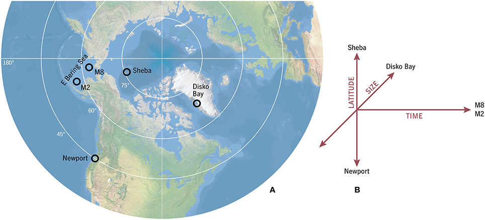
Figure 1. (A) Locations of model testbeds. The “global” model experiment spans a gradient from approximately Ice Station Sheba to Newport, Oregon, and beyond. This experiment and the Bering Sea and Disko Bay testbeds constitute (B) a complementary set examining variation in space, time, and size diversity.

The first of these criteria, captured by a Disko Bay, West Greenland model experiment (Figure 1, Section 3.4) is central to the goal of eventually allowing climate-to-copepod model studies to replace hand-picked sets of fixed types with a trait continuum. The second and third criteria (captured by a Bering Sea hindcast experiment and an heuristic, idealized biogeographic experiment: Figure 1, Sections 3.2, 3.3) provide complementary constraints on the parameterization of individual energetics, and help distinguish the effects of temperature and prey seasonality. As we will show, these initial experiments suggest a general hypothesis: that the viability of the calanoid community, at least near its high-latitude limit, is much more sensitive to prey abundance and phenology than to temperature.

2. Model Description

2.1. General Approach

The model introduced here is “Coltrane” (Copepod Life-history Traits and Adaptation to New Environments) version 1.0. Matlab source code is available at https://github.com/neilbanas/coltrane. An overview of the model structure is shown in Figure 2.

FIGURE 2

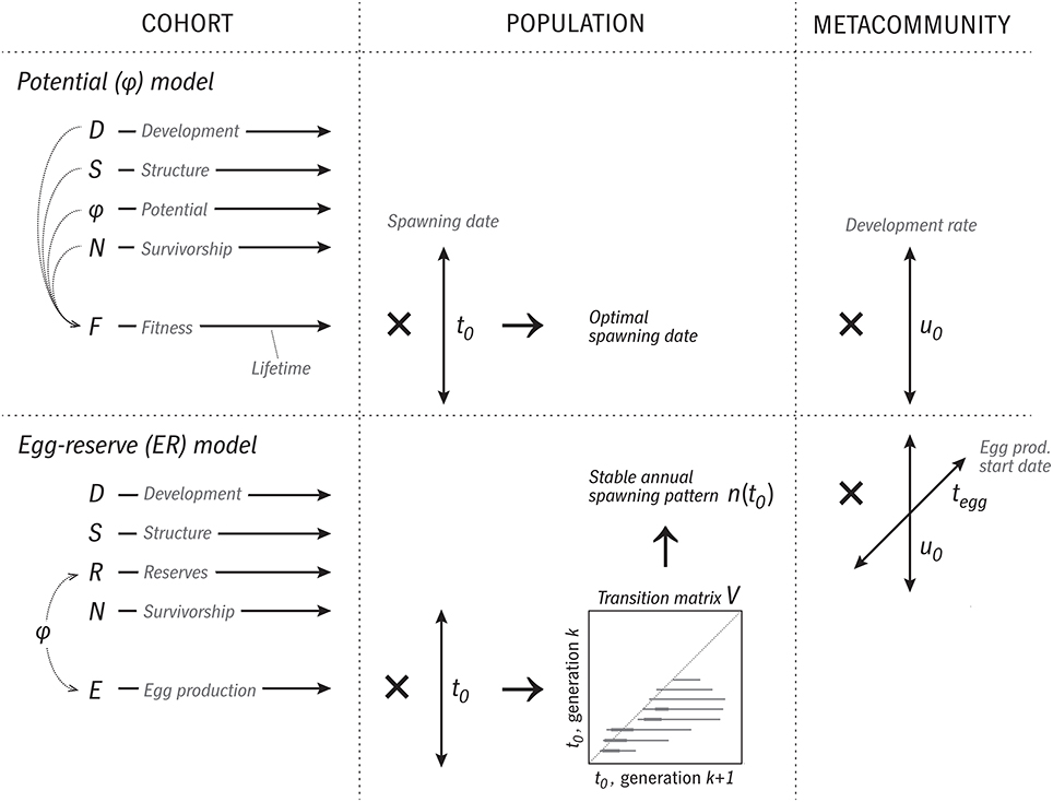
Figure 2. Overview of the logic and execution of the two versions of the Coltrane 1.0 model. In the φ version, a cohort is represented by four state variables (D, S, φ, N) integrated forward in time over the cohort's lifespan. These are used to calculate a time series of fitness F. Next, this calculation is repeated across a family of spawning dates t₀, and optimal and viable t₀ cases determined. This constitutes a population-level description, which then can be repeated across a range of trait values (u₀, relative development rate) to describe a size-variable metacommunity. In the ER version, at the cohort level, φ is replaced by the state variable R and a time series of egg production E. Across a family of t₀ cases, a transition-matrix method is used to determine a stable annual pattern of relative egg production n(t₀), which is taken as the population-level prediction. A metacommunity is formed by varying two traits, u₀ and the date at which egg production begins t_egg.

Like many individual-based models, Coltrane represents the time-evolution of one cohort of a clonal population, all bearing the same traits and spawned on the same date t₀, with a set of ODEs. The state variables describing a cohort are relative developmental stage D, where D = 0 represents a newly spawned egg and D = 1 an adult; survivorship N, the fraction of initially spawned individuals that remain after some amount of cumulative predation mortality; structural biomass per individual S, and “potential” or “free scope” φ, which represents all net energy gain not committed to structure, or equivalently, the combination of internal energy reserves and eggs already produced. Combining reserves and eggs into one pool in this way lets us cleanly separate results that depend only on the fundamental energy budget (gain from ingestion, loss to metabolism, and energy required to build somatic structure) from results that depend on particular assumptions about egg production (costs, cues, and strategies). An alternate form of the model explicitly divides φ into internal reserves R and egg production rate E: the simpler model without this distinction will be called the “potential” or φ model and the fuller version the “egg/reserve” or ER model.

The φ and ER models take different approaches to generating population-level results from this cohort model, as explained in detail below (Section 2.4). In both cases, the logic changes from the simple forward time-integration at the cohort level: one runs the cohort model for all possible spawning dates t₀, retroactively determines which spawning dates would prove optimal or sustainable, and considers the cohort time series from those t₀ values, appropriately weighted, to constitute the model solution (Section 2.4). The biological logic here is similar to the backwards-in-time dynamical optimization method frequently used in studies of optimal annual routines (Houston et al., 1993; Varpe et al., 2007), although our solving method is quite different and less exact. This is a compromise with the eventual goal of coupling Coltrane to oceanographic models as a spatially explicit IBM.

Communities are generated in Coltrane 1.0 simply by running families of cases of the population-level model that vary one or more traits. Treating coexisting populations as uncoupled vastly simplifies the interpretation of the landscape of viable strategies in a given environment, or the fundamental niche of a particular trait combination, our primary modes of analysis. At the same time, it tightly restricts our choices regarding the formulation of predation mortality. In reality, coupling through shared predators can rival bottom-up effects as a determinant of community structure (Holt et al., 1994; Chesson, 2000; Record et al., 2013, 2014), and we expect that many potential applications of this model would require that this be better represented. In the present study, we have taken the minimalist, incrementalist approach of imposing the simplest possible form of predation mortality—a linear function, with scalings that closely mirror the growth and development functions (Section 2.2)—and restricting the terms of analysis. In particular, we will describe model output in terms of trait correlations, optimality, and viability, but not in terms of absolute copepod biomass or abundance. Likewise, while some plankton models resolve the process of adaptation explicitly (Clark et al., 2013), we address it only in the indirect sense of mapping the viable and optimal regions of the strategy landscape. This approach is less mechanistic but also helpfully agnostic about whether adaptation in the copepods arises through individual plasticity, species composition shifts, or natural selection per se.

An environment in Coltrane 1.0 is defined by annual cycles of three variables, total concentration of phytoplankton/microzooplankton prey P, surface temperature T₀, and deep temperature T_d. At present, these annual cycles are assumed to be perfectly repeatable, so that a “viable” strategy can be defined as a set of traits that lead to annual egg production above the replacement rate, given P, T₀, and T_d as functions of yearday t. The level of predation mortality (Section 2.2.4) might also be viewed as an environmental characteristic.

2.2. Time Evolution of One Cohort

2.2.1. Ontogenetic Development

Calanoid copepods have a determinate developmental sequence, comprising the embryonic period, six naupliiar stages (N1–6), five copepodid stages (C1–5), and adulthood (C6). Similar to Maps et al. (2012), conversions between relative developmental stage D and the actual 13-stage sequence have been done using relative stage durations for C. finmarchicus from Campbell et al. (2001), which appear to be appropriate for other Calanus spp. with the proviso that C5 duration is particularly variable and strategy-dependent. Development in the model follows

$\begin{array}{ll}\frac{dD}{dt}=u,D\le 1& (1)\end{array}$

where developmental rate u is

$\begin{array}{ll}u=a{q}_d\sigma u_0& (2)\end{array}$

and

$\begin{array}{ll}{q}_d\equiv Q_d^{T/10^{°}\mathrm{\text{C}}}& (3)\end{array}$

$\begin{array}{ll}T=a{T}_0+(1-a)T_d& (4)\end{array}$

$\begin{array}{ll}\sigma \equiv \frac{P}{K_{s}P}& (5)\end{array}$

All variables and parameters are defined in Table 1. Activity level a is, in this version of the model, a two-state switch calculated at each time step, 1 during active feeding and 0 during diapause. The temperature-dependent factor q_d describes a power-law response with a Q₁₀ of Q_d, where temperature is assumed to be T₀ during active feeding and T_d during diapause. We use the Q₁₀ functional form for convenience: the differences between this and the leading alternatives (Belěhrádek, Arrhenius: Forster et al., 2011; Record et al., 2012) appear to be small compared with interspecies differences in this study (Banas and Campbell, 2016). Prey saturation σ is a simple Michaelis–Menten function with half-saturation K_s. The parameter u₀, the development rate corrected to 0°C, was found by Banas and Campbell (2016) to be the primary trait responsible for differences in adult body size among Calanus spp. and other calanoids >50 μg C adult size, although not at a broader scale of diversity. It represents the aspect of development-rate variation that we interpret to be a strategy choice as opposed to a physiological or thermodynamic constraint.

TABLE 1

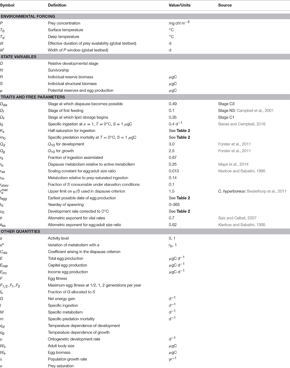
Table 1. Parameter values and other symbols used in the manuscript.

2.2.2. Energy Gain and Loss

The two energy stores S (structure) and φ (reserves/potential) follow

$\begin{array}{ll}\frac{dS}{dt}=f_{s}GS& (6)\end{array}$

$\begin{array}{ll}\frac{d\phi }{dt}=(1-f_s)GS& (7)\end{array}$

where G is net energy gain (ingestion minus metabolic losses). When net gain is positive, it is allocated between structure and potential according to the factor f_s, which commits net gain entirely to structure before a developmental point D_s, entirely to potential during adulthood, and to a combination of them in between:

$\begin{array}{ll}{f}_s=\{\begin{array}{ll}1,\hfill & D<D_s\hfill \\ \frac{1-D}{1-D_s},\hfill & D_s\le D\le 1\hfill \\ 0,\hfill & D=1\hfill \end{array}& (8)\end{array}$

When G ≤ 0, the deficit is taken entirely from reserves: f_s = 0.

Before the first feeding stage (D < D_f) we assume G = 0 for simplicity. After feeding begins,

$\begin{array}{ll}G=r_{a}I-M& (9)\end{array}$

where ingestion I and metabolic loss M are given by

$\begin{array}{ll}I=a\sigma q_g{I}_0{S}^{\theta -1}& (10)\end{array}$

$\begin{array}{ll}M=a^{\star }{r}_m{q}_g{I}_0{S}^{\theta -1}& (11)\end{array}$

and r_a is an assimilation efficiency. Ingestion follows a Kleiber's Law-like dependence on structural body mass S, with θ = 0.7 (Kleiber, 1932; Saiz and Calbet, 2007). I₀ is specific ingestion rate at saturating prey concentration, T = 0°C, and S = 1 μg C. This is modulated by the activity switch a and prey saturation σ as in Equation (2), and a power-law temperature response for growth

$\begin{array}{ll}{q}_g\equiv Q_g^{T/10^{°}\mathrm{\text{C}}}& (12)\end{array}$

which is parallel to that for development (q_d) but with a different Q₁₀. Q₁₀ values have been found to vary among copepod species but Banas and Campbell (2016) argue that common values derived from a fit across community-level data are more appropriate for comparing species near their thermal optima. We use Q_g = 2.5 and Q_d = 3.0, as an approximation to the best-fit complex allometric curves reported by Forster et al. (2011).

Energy loss to metabolism M follows the same temperature and size scalings. The factor r_m is the ratio of metabolism to ingestion when prey is saturating. Unlike development and ingestion, which are assumed zero during diapause, M during diapause is nonzero but reduced to a basal fraction r_b ≈ 1/4 (Maps et al., 2014):

$\begin{array}{ll}{a}^{\star }=r_b+(1-r_b)a& (13)\end{array}$

Note that in this formalism, gross growth efficiency ϵ becomes

$\begin{array}{ll}ϵ=\frac{G}{I}=r_a-\frac{r_m}{\sigma }& (14)\end{array}$

when a = 1. We have set r_m = 0.14 such that ϵ = 0 when P = 1/4 K_s.

2.2.3. Starvation

Potential φ is allowed to run modestly negative, to represent consumption of body structure during starvation conditions. A cohort is terminated by starvation if

$\begin{array}{ll}\phi <-r_{starv}S& (15)\end{array}$

where in this study r_starv = 0.1. A convenient numerical implementation of this scheme is to integrate S implicitly so that it is guaranteed > 0, and to integrate φ explicitly so that it is allowed to change sign, with no change of dynamics at φ = 0.

2.2.4. Predation Mortality

Predation mortality is assumed to have the same dependence on temperature and body size as ingestion, metabolism, and net gain (Hirst and Kiørboe, 2002). Survivorship N is set to 1 initially and decreases according to

$\begin{array}{ll}\frac{d(lnN)}{dt}=-m& (16)\end{array}$

(it is convenient to calculate the numerical solution using ln N rather than N as the state variable, since values become extremely small). The mortality rate m is

$\begin{array}{ll}m=a{q}_g{S}^{\theta -1}{m}_0& (17)\end{array}$

such that that predation pressure relative to energy gain is encapsulated in a single parameter m₀. In practice m₀ is a tuning parameter but we can solve for the value that would lead to an approximate equilibrium between growth and mortality. The condition

$\begin{array}{ll}\frac{1}{NS}\frac{d(NS)}{dt}=0& (18)\end{array}$

is equivalent, by Equations (6) and (16), to

$\begin{array}{ll}m=f_{s}G& (19)\end{array}$

and with a = 1 this becomes

$\begin{array}{ll}\frac{m_0}{I_0}=(r_a\sigma -r_m)f_s& (20)\end{array}$

Averaging f_s over the maturation period 0 ≤ D ≤ 1 with D_s = 0.35, and assuming σ ≈ 2/3 on average for an organism that has aligned its development with the productive season, gives m₀ ≈ 0.2 I₀. This is the default level of predation in the model except where otherwise specified.

2.2.5. Activity Level and Diapause

Modulation of activity level a has been treated as simply as possible, using a “myopic” criterion that considers only the instantaneous energy budget, rather than an optimization over the annual routine or lifetime (Sainmont et al., 2015). Furthermore, we treat a as a binary switch—diapause or full foraging activity—although intermediate overwintering states have been sometimes observed, e.g., C. glacialis/marshallae on the Eastern Bering Sea shelf in November (Campbell, personal communication). In the present model, we set a = 0 if D > D_dia (the stage at which diapause first becomes possible) and the environment is such that total population energy gain

$\begin{array}{ll}\frac{d}{dt}(\phi +S)N=(GS)N& (21)\end{array}$

would be higher under diapause. We can derive an expression for the threshhold at which this occurs by maximizing population energy gain as a function of a. When d/da of GSN is positive, active foraging a = 1 is the optimal instantaneous strategy and when it is negative, a = 0 is optimal. The threshhold

$\begin{array}{ll}\frac{d}{da}(GSN)=0& (22)\end{array}$

can be rearranged to give a critical prey-saturation level

$\begin{array}{ll}{\sigma }_{crit}=\frac{r_m(1-r_b)}{r_a}+\frac{C_{dia}}{r_a}\frac{m_0}{I_0}& (23)\end{array}$

where C_dia = 1 + φ/S. The first term in Equation (23) can be derived more simply by setting dG/da = 0, a criterion based on ingestion and metabolism alone. The second term adjusts this criterion by discouraging foraging at marginal prey concentrations when predation is high. A third, temperature-dependent term has been neglected. The second, mortality-dependent term tends to produce unrealistic, rapid oscillations in which the copepods briefly “top up” on prey and then hide in a brief “diapause” to burn them. It is unclear whether this model behavior is a mathematical artifact—a limitation of combining actual lipid reserves and potential egg production into a single state variable—or whether it suggests that under some conditions the optimal level of foraging is intermediate between full activity and none. Incorporating a more mechanistic treatment of optimal foraging (Visser and Fiksen, 2013) and allowing a to vary continuously would address this. In this study, we have eliminated the phenomenon by approximating C_dia as

$\begin{array}{ll}{C}_{dia}=max\left[0,1+min\left({\displaystyle r_{\phi }^{max}},\frac{\phi }{S}\right)\right]& (24)\end{array}$

where $r_{\phi }^{max}=1.5$.

2.3. Eggs and Potential Eggs

The evolution equations above Equations (1), (6), (7), (16) specify the development of one cohort in the φ model. If this model is elaborated with an explicit scheme for calculating total egg production over time E(t), then it is possible to define R(t), individual storage/reserve biomass, and interpret R as a state variable and φ as a derived quantity. The relationship between the two is

$\begin{array}{ll}\frac{dR}{dt}=(1-f_s)GS-E& (25)\end{array}$

$\begin{array}{ll}\phi (t)=R(t)+{\displaystyle {\int }_{t_0}^t}E(t^{\prime })d{t}^{\prime }& (26)\end{array}$

Thus, φ tracks the reserves that an animal would have remaining if it had not previously started egg production. This is a useful metric for optimizing reproductive timing, as we will show (Section 2.4).

Any explicit expression for E(t) allows Equation (25) to replace Equation (7). In one model experiment below (Section 3.4), we use the following scheme: E(t) is the sum of income egg production E_inc and capital egg production E_cap, which are 0 until maturity is reached (D = 1) and an additional timing threshhold has been passed (t > t_egg). Past those threshholds, they are calculated as

$\begin{array}{ll}\begin{array}{ll}{E}_{inc}=G,& G>0\\ E_{cap}=E_{max}-E_{inc},& D>0\end{array}& (27)\end{array}$

where E_max is a maximum egg production rate which we assume to be equal to food-saturated assimilation:

$\begin{array}{ll}{E}_{max}=r_a{q}_g{I}_0{S}^{\theta }& (28)\end{array}$

Thus, the trait t_egg determines whether egg production begins immediately upon maturation (if t_egg is prior to the date on which D reaches 1) or after some additional delay. Instead of t_egg, expressed in terms of calendar day, one could introduce the same timing freedom through a trait linked to light, an ontogenetic clock that continues past D = 1, or a more subtle physiological scheme. However, since we run a complete spectrum of trait values in each environmental case, it is not important to the results how the delay is formulated, provided we only compare model output, rather than actual trait values, across cases.

2.4. Population-Level Response

A population-level simulation (Figure 2) consists of integrating either the φ model (Equations 1, 6, 7, 16) or ER model (Equations 1, 6, 16, 25) for a full annual cycle of spawning dates t₀, and then identifying optimal and viable values of t₀ in terms of the egg fitness F, future egg production per egg (Varpe et al., 2007). Calculating a time series of F in the φ model requires an estimate of individual egg biomass W_e in order to convert φ(t) from carbon units into a number of eggs, and a similar issue arises in the ER population model. Thus, a digression on the determination of W_e is required.

2.4.1. Egg and Adult Size

The problem of estimating W_e can be replaced by the problem of estimating adult size W_a using the empirical relationship for broadcast spawners determined by Kiørboe and Sabatini (1995):

$\begin{array}{ll}ln{W}_e\approx ln{r}_{ea}+{\theta }_{ea}ln{W}_a& (29)\end{array}$

where r_ea = 0.013, θ_ea = 0.62 (In the ER model, W_a ≡ S + R at D = 1, but in the φ model we approximate it as S alone for simplicity). Adult size itself is an important trait for the model to predict, but the controls on it are rather buried in the model formulation above. Banas and Campbell (2016) describe a theory relating body size to the ratio of development rate to growth rate based on a review of laboratory data for copepods with adult body sizes 0.3–2000 μgC. In our notation, their model can be derived as follows: if we approximate Equations (6), (7) in terms of a single biomass variable as

$\begin{array}{ll}\frac{dW}{dt}={ϵ}^{\prime }{q}_g{I}_0{W}^{\theta },D\ge D_f& (30)\end{array}$

then integrating from spawning to maturation gives

$\begin{array}{ll}{\frac{1}{1-\theta }{W}^{1-\theta }|}_{D=0}^{D=1}=(1-D_f){ϵ}^{\prime }{q}_g{I}_0\frac{1}{u}& (31)\end{array}$

since u is the reciprocal of the total development time. Growth rate has been written in terms of I₀ and an effective growth efficiency over the development period ϵ′. If we assume that egg biomass W_e = W|_{D = 0} is much smaller than W_a = W|_{D = 1}, then combining Equation (31) with Equation (2) gives

$\begin{array}{ll}{W}_a\approx {\left[(1-\theta )(1-D_f){ϵ}^{\prime }{\left(\frac{Q_g}{Q_d}\right)}^{T/{10}^{°}\text{C}}\frac{I_0}{u_0}\right]}^{\frac{1}{1-\theta }}& (32)\end{array}$

Properly speaking, both ϵ′ and T in Equation (32) are functions of t₀ since they depend on the alignment of the development period with the annual cycle. Since we are trying to use Equations (29), (32) to optimize t₀, we have a circular problem. Record et al. (2013) derive an expression similar to Equation (32) and apply it iteratively because of this circularity. Some applications of Coltrane might require the same level of accuracy, but in the present study we take the expedient approach of simply assuming that T is the annual mean of T₀ and that ϵ′ ≈ 1/3: i.e., that after t₀ is optimized, some diapause/spawning strategy will emerge that aligns the maturation period moderately well with a period of high prey availability. This assumption eliminates the need to run the model before estimating W_e via Equations (29), (32).

2.4.2. Optimal Timing in the φ Model

With a method for approximating W_e in hand, we can define egg fitness F as a function of φ. If a cohort spawned on t₀ were to convert all of its accumulated free scope φ—all net energy gain beyond that required to build an adult body structure—into eggs on a single day t₁, the eggs produced per starting egg would be

$\begin{array}{ll}F(t_0\to t_1)=\frac{\phi (t_1)}{W_e}N(t_1)& (33)\end{array}$

This expression condenses one copepod generation into a mapping F similar to the “circle map” of Gurney et al. (1992). Once the ODE model has been run for a family of t₀ cases, this mapping can be used to quickly identify optimal life cycles of any length. The optimal one-generation-per-year strategy is the t₀ that maximizes F₁ = F(t₀ → t₀ + 365). The optimal one-generation-per-two-years strategy has t₀ that maximizes F_1/2 = F(t₀ → t₀ + 2 · 365). The optimal two-generation-per-year strategy has spawning dates t₀, t₁ that maximize the product F₂ = F(t₀ → t₁) · F(t₁ → t₀ + 365); and so on. A viable strategy is a combination of spawning dates and model parameters that give F ≥ 1.

2.4.3. Optimal Timing in the ER Model

In reality, of course, copepods are not free to physically store indefinite amounts of reserves within their bodies and then instantaneously convert them into eggs when the timing is optimal. If a scheme for calculating egg production over time E(t) is added to the model as in Section 2.3, then the per-generation mapping represented by F takes a different form. First, for each cohort, we use the assumption that the environmental annual cycle repeats indefinitely to convert the time series of EN—egg production discounted by survivorship—to a function of yearday, by adding the value on days 365+i, 2·365+i, … to the value on day i (in practice we discretize the year into 5 d segments rather than yeardays per se). Next, we construct a matrix V whose rows are the year-long time series of EN/W_e for each spawning date t₀. V is thus a transition matrix with spawning date in generation k running down rows and spawning date in generation k + 1 running across columns. Given a discrete annual cycle n_k of eggs spawned in generation k, one can calculate the expected annual cycle of egg production in the next generation as n_k+1 = V · n_k, where n is given as a column vector.

The first eigenvector of V gives a seasonal pattern of egg production that is stable in shape, with the corresponding eigenvalue λ giving one plus the population growth rate per generation:

$\begin{array}{ll}{n}_{k+1}(t)=V·n_k(t)=\lambda n_k(t)& (34)\end{array}$

$\begin{array}{ll}\frac{n_{k+1}(t)-n_k(t)}{\mathrm{\text{1 generation}}}\approx \lambda -1& (35)\end{array}$

A strict criterion for strategy viability would then be λ ≥ 1, although this criterion is unhelpfully sensitive to predation mortality. A more robust criterion (which we use in Section 3.4 below) is to consider a strategy viable if it yields lifetime egg production above the replacement rate: if E(t₀; t) and N(t₀; t) are the time series of egg production and survivorship for a cohort spawned on t₀, and n(t₀) is a normalized annual cycle of egg production,

$\begin{array}{ll}{\displaystyle {\int }_0^{365}}{\displaystyle {\int }_0^{\infty }}n(t_0)\frac{E(t_0;t)N(t_0;t)}{W_e}dtd{t}_0\ge 1& (36)\end{array}$

Thus, in the ER version of the model, as in the φ version, we have an efficient method that describes the long-term viability of a trait combination under a stable annual cycle, along with the optimal spawning timing associated with those traits in that environment; and these methods only require us to explicitly simulate one generation.

2.5. Assembling Communities

Community-level predictions in Coltrane take the form of bounds on combinations of traits that lead to viable populations in a given environment (Figure 2). There are many copepod traits represented in the model that one might consider to be axes of diversity or degrees of freedom in life strategy: u₀, I₀, θ, D_s, K_s, W_e/W_a, and even m₀ to the extent that predation pressure is a function of behavior (Visser et al., 2008). Record et al. (2013) allowed five traits to vary among competitors in their copepod community model. We have taken a minimalist approach, where in the φ model we allow only one degree of freedom: variation in u₀ from 0.005 to 0.01 d⁻¹. Banas and Campbell (2016) showed from a review of lab studies that u₀ variations appear to be the primary mode of variation in adult size among large calanoids (W_a > 50 μgC) including Calanus and Neocalanus spp., with slower development leading to larger adult sizes. That study also suggests that variation in I₀ is responsible for copepod size diversity on a broader size or taxonomic scale (e.g., between Calanus and small cyclopoids like Oithona). However, variation in I₀ (energy gain from foraging) probably only makes sense as part of a tradeoff with predation risk or egg survivorship (Kiørboe and Sabatini, 1995) and we have left the formulation of that tradeoff for future work. We therefore expect Coltrane 1.0 to generate analogs for large and small Calanus spp. (~100–1000 μgC adult size) but not analogs for Oithona spp. or even small calanoids like Pseudocalanus or Acartia.

Choices regarding reproductive strategy require another degree of freedom. In the φ model, this does not require additional parameters, because the difference between, e.g., capital spawning in winter and income spawning in spring is simply a matter of the time t at which F is evaluated in postprocessing: each model run effectively includes all timing possibilities (Equation 33). In the ER model, however, diversity in reproductive timing must be made explicit. Under the simple scheme for egg production specified above (Section 2.3), this takes the form of running a family of cases varying t_egg for each t₀ and u₀.

2.6. Model Experiments

This study comprises three complementary experiments (Table 2). The first of these is an idealized global testbed which addresses broad biogeographic patterns. The second is a testbed representing the Eastern Bering Sea shelf, which addresses time-variability in one population in one environment. The last is a testbed representing Disko Bay, West Greenland, which addresses trait relationships along the size spectrum in detail. The first two are evaluated entirely in terms of the φ model, while in the Disko Bay case we use the ER model to allow more specific comparisons with observations.

TABLE 2

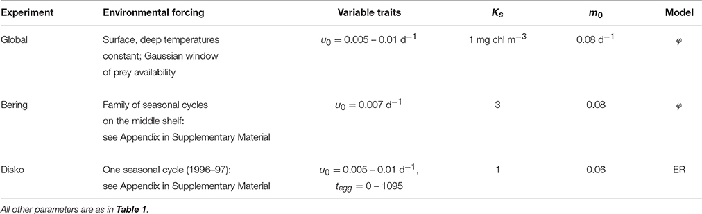
Table 2. Setup of model experiments.

The global testbed consists of a family of idealized environments in which surface temperature T₀ is held constant, and prey availability is a Gaussian window of width δt′ centered on yearday 365/2:

$\begin{array}{ll}P(t)=({10\text{mg chl m}}^{-3})exp\left[-{\left(\frac{t-\frac{365}{2}}{\delta t^{\prime }}\right)}^2\right]& (37)\end{array}$

We compare environmental cases in terms of T₀ and an effective season length

$\begin{array}{ll}\delta t={\displaystyle {\int }_0^{365 \mathrm{\text{d}}}}\sigma dt& (38)\end{array}$

which rescales the δt′ cases in terms of the equivalent number of days of saturating prey per year. We assume that deep, overwintering temperature T_d = 0.4 T₀. The ratio 0.4 matches results of a regression between mean temperature at 0 and 1000 m in the Atlantic between 20 and 90°N, or 0 and 500 m in the Northeast Pacific over the same latitudes (World Ocean Atlas 2013: http://www.nodc.noaa.gov/OC5/woa13/). Over the same data compilation, the mean seasonal range in temperature is approximately 5°C at the surface (and approximately zero at 500–1000 m); an alternate formulation of the testbed that models T₀ as an annual sinusoid with this range gives results that are somewhat noisier but heuristically very similar to those shown in Section 3.2 below.

The Bering Sea testbed considers interannual variation in temperature, ice cover, and the effect of ice cover on in-ice and pelagic phytoplankton production (Stabeno et al., 2012b; Sigler et al., 2014; Banas et al., 2016). Variation between warm, low-ice years and cold, high-ice years has previously been linked to the relative abundance of large zooplankton including C. glacialis/marshallae (Eisner et al., 2014), and we test Coltrane predictions against 8 years of C. glacialis/marshallae observations from the BASIS program. Seasonal cycles of T₀, T_d, and P are parameterized using empirical relationships between ice and phytoplankton from Sigler et al. (2014) and a 42-year physical hindcast using BESTMAS (Bering Ecosystem Study Ice-ocean Modeling and Assimilation System: Zhang et al., 2010; Banas et al., 2016). Details are given in the Appendix in Supplementary Material.

The Disko Bay testbed represents one seasonal cycle of temperature and phytoplankton and microzooplankton prey, based on the 1996–1997 time series described by Madsen et al. (2001). We use this particular dataset not primarily as a guide to the current or future state of Disko Bay but rather as a specific circumstance in which the life-history patterns of three coexisting Calanus spp. (C. finmarchicus, C. glacialis, C. hyperboreus) were documented (Madsen et al., 2001). Details are given in Section 3.4 and the Appendix in Supplementary Material.

3. Results

3.1. An Example Population

One case from the global experiment with u₀ = 0.007 d⁻¹, T₀ = 1°C, and δt = 135 is shown in detail in Figure 3 to illustrate the analysis method described in Section 2.4.2. In this case, out of cohorts spawned over the full first year, only those spawned in spring reached adulthood without starving (Figure 3B, blue–green lines; non-viable cohorts not shown). The fitness function F (Equation 42) declines during winter diapause and rises during the following summer when prey are available. There is no equivalent peak during the third summer, indicating that by this time cumulative predation mortality is so high that there is no net advantage to continuing to forage before spawning.

FIGURE 3

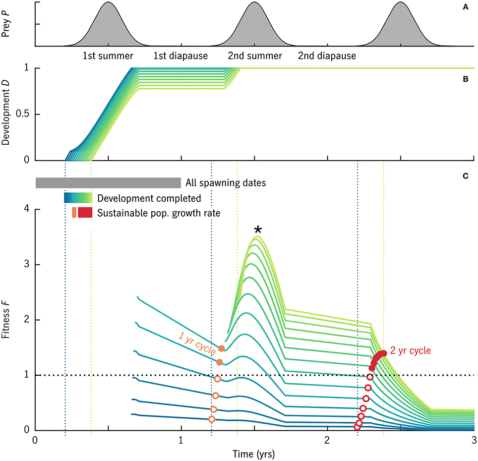
Figure 3. Results of an example model case with u₀ = 0.007 d⁻¹, T₀ = 1°C, and δt = 135. Cohorts were simulated beginning from all spawning dates in year 1. (A) Prey availability over time. (B) Developmental stage D for cohorts that reach maturity (D = 1) without starving: the blue–yellow color scale corresponds to spawning dates t₀ over the viable period from pre-bloom to bloom maximum. (C) Fitness F over time for the cohorts shown in (B), i.e., the expected value (eggs egg⁻¹) of converting all free scope φ to eggs on a given date. Curves of F begin when maturity is reached (D = 1) and egg production becomes possible. Open and solid circles mark the value of F on the 1-year (orange) and 2-year (red) anniversaries of the original spawning date. Solid circles mark cohorts that achieve a fitness above the replacement rate.

The maximum value of F for most cohorts (*, Figure 3C) comes at ~1.5 year into the simulation, at the peak in prey availability following maturation. This point in the annual cycle, however, does not fall within the window of spawning dates at which maturation is possible (compare year 2 in Figure 3C with year 1 in Figure 3B), and thus is an example of “internal life history mismatch” (Varpe et al., 2007), the common situation in which the spawning timing that maximizes egg production by the parent is not optimal for the offspring. The long-term egg fitness corresponding to stable 1-year and 2-year cycles is marked for each cohort (Figure 3C, red, orange circles). Some but not all of the cohorts that reach maturity are able to achieve F > 1, egg production above the replacement rate, in these cyclical solutions (solid circles). The best 1-year and 2-year strategies achieve similar maximum fitness values (red vs. orange solid dots), although they require slightly different seasonal timing.

Note that although F can be described as the egg-fitness function, the lines in Figure 3C—time series of F for particular spawning dates t₀—are not the same as the seasonal curve of egg fitness that results from a backwards-in-time dynamic optimization (e.g., Figure 6F in Varpe et al., 2007). Rather, each curve of F(t₀; t) in our approach gives a series of possible values for egg fitness at t₀ depending on what future strategy is taken. The forwards and backwards calculations converge (at least qualitatively) once the internal life-history mismatch is resolved and a stable long-term cycle is found (red and orange circles, Figure 3C). As expected (Varpe et al., 2007), these stable values of egg fitness peak, for each generation length, somewhat prior to the bloom maximum (Figure 3C).

3.2. Global Behavior

In the global experiment, populations like that shown in Figure 3 were run for a spectrum of u₀ values, across combinations of T₀ and δt from −2 to 16°C and 0 to 310 d (the latter corresponding to δt′ from 0 to 150 d). Across these cases, at a given u₀, the model predicts a log-linear relationship between adult size and temperature, which is not much perturbed by variation in prey availability (Figure 4). The slope of this relationship is equivalent to a Q₁₀ of 1.8–2.0, consistent with that predicted by Equation (32):

$\begin{array}{ll}{\left(\frac{Q_d}{Q_g}\right)}^{\frac{1}{1-\theta }}\approx 1.84& (39)\end{array}$

FIGURE 4

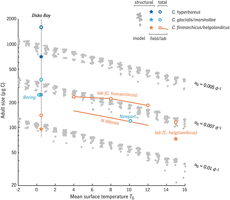
Figure 4. Relationship between adult size W_a and mean surface temperature T₀ in the “global” model experiment, for three values of relative development rate u₀, in comparison with observations (Peterson, 1986; Swalethorp et al., 2011; Wilson et al., 2015; Campbell et al., in press) and laboratory results (Campbell et al., 2001; Rey-Rassat et al., 2002). Model results (gray dots) represent structural biomass S, as do observations marked with a ⋆; observations marked with a ◦ represent total biomass R + S. Clusters of gray dots indicate families of model cases varying productive season length (horizontal axis in Figure 5).

Field observations of size in relation to temperature in C. finmarchicus and C. helgolandicus across the North Atlantic show a similar relationship (Q₁₀ = 1.65, Wilson et al., 2015, with prosome length converted to carbon weight based on Runge et al., 2006). Somewhat surprisingly, even wide variation in prey conditions (clusters of gray dots, Figure 4) has only minor effects on this slope.

The intercept of the size-temperature relationship depends on u₀ (Figure 4), with u₀ = 0.005–0.01 d⁻¹ corresponding to the range of adult size from C. finmarchicus to C. hyperboreus at the cold end of the temperature spectrum (Disko Bay, ~0°C: Swalethorp et al., 2011). It is not always fair, however, to associate a particular u₀ value with a particular species over the full range of temperatures included. As Banas and Campbell (2016) discuss further, the temperature response of an individual species is often dome-shaped, a window of habitat tolerance (Møller et al., 2012; Alcaraz et al., 2014), whereas Coltrane 1.0 uses the monotonic, power-law response observable at the community level (Forster et al., 2011). C. finmarchicus, for example, is fit well by u₀ = 0.007 d⁻¹ at higher temperatures (4–12°C), whereas near 0°C in Disko Bay, it has been observed to be considerably smaller than extrapolation along the u₀ = 0.007 d⁻¹ power law would predict. Past studies have also found C. finmarchicus growth and ingestion to be suppressed at low temperatures, i.e., to show a very high Q₁₀ compared with the community-level value (Campbell et al., 2001; Møller et al., 2012).

With this caveat on the interpretation of u₀, we can observe a sensible gradation in life strategy along the u₀ axis (Figure 5). From u₀ = 0.01 d⁻¹ (C. finmarchicus-like at 0°C) to u₀ = 0.005 d⁻¹ (C. hyperboreus-like), the environmental window in which multi-year life cycles are viable (F_1/2 ≥ 1) expands dramatically. This window overlaps significantly with the window of viability for 1-year life cycles (F₁ ≥ 1; Figure 5, black vs. gray contours). In all u₀ cases, there is a non-monotonic pattern in maximum fitness as a function of either temperature or prey (Figure 5, color contours), as environments align and misalign with integer numbers of generations per year or years per generation.

FIGURE 5

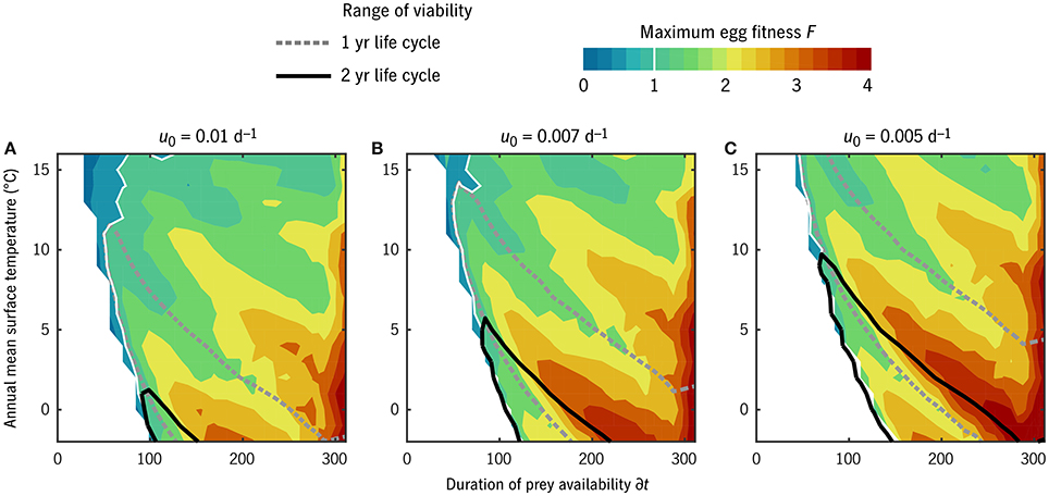
Figure 5. Maximum egg fitness (eggs per starting egg per generation) across all combinations of temperature and duration of prey availability in the “global” experiment. Unfilled contour lines give the environmental range over which 1-year (gray, dotted) and 2-year (black, solid) life cycles are viable. The white regions at low prey availability indicate environments in which no timing strategy exists that allows successful maturation. (A–C) Give results for three values of u₀ corresponding to the families of cases shown in Figure 4.

The overall gradient from high to moderate F with increasing temperature (Figure 5) is largely an artifact of displaying F normalized to generation as opposed to per calendar year. In general, these results should not be taken as a quantitative prediction of annual production rates: the linear mortality closure that simplifies the analysis also omits the role of density dependence in stabilizing growth rates. Accordingly, in what follows, we consider only whether F in a given circumstance exceeds replacement rate, not whether it exceeds it modestly or dramatically.

The number of generations per year in the timing strategy that optimizes F for each (T₀, δt) habitat combination is shown in Figure 6 for u₀ = 0.007 d⁻¹. This u₀ value corresponds in adult size to Arctic C. glacialis and temperate C. marshallae populations in the Pacific (Figure 4), species which coexist and are nearly indistinguishable in the Bering Sea. In the lowest-prey conditions, no timing strategy is found to be viable. As prey and temperature increase, the model predicts bands proceeding monotonically from multiple years per generation to multiple generations per year. Validating these model predictions requires parameterizing places (in terms of T₀ and δt) in addition to parameterizing their inhabitants, and thus the meaning of either success of failure is ambiguous. Still, we can observe the following. Ice Station Sheba in the high Pacific Arctic (Figure 1) falls in the non-viable regime (Figure 6), consistent with the conclusion of Ashjian et al. (2003) that Calanus spp. are unable to complete their life cycle there. Disko Bay falls on the boundary of 1- and 2-year generation lengths, consistent with observations of C. glacialis there (Madsen et al., 2001). At Newport, Oregon, near the southern end of the range of C. marshallae, the model predicts multiple generations per year, consistent with observations by Peterson (1979).

FIGURE 6

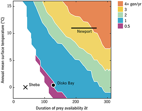
Figure 6. Generations per year of the optimal strategy in each environmental combination for relative development rate u₀ = 0.007 d⁻¹ (C. glacialis/marshallae analogs). Ice Station Sheba, Disko Bay, and Newport (Figure 1) have been placed approximately for comparison.

3.3. A High-Latitude Habitat Limit in Detail: The Eastern Bering Sea

These idealized experiments (Figures 5, 6) suggest that very short productive seasons place a hard limit on the viability of Calanus spp., regardless of size, temperature, generation length, or match/mismatch considerations (although these factors affect where exactly the limit falls). A decade of observations in the Eastern Bering Sea provide a unique opportunity to resolve this viability limit with greater precision. This analysis takes advantage of the natural variability on the Southeastern Bering Sea shelf described by the “oscillating control hypothesis” of Hunt et al. (2002, 2011): in warm, low-ice years, the spring bloom in this region is late (~ yearday 150; Sigler et al., 2014) and the abundance of large crustacean zooplankton including C. glacialis/marshallae is very low, while in colder years with greater ice cover, the pelagic spring bloom is earlier, ice algae are present in late winter, and large crustacean zooplankton are much more abundant. The task of replicating these observations serves to test the Coltrane parameterization, and situating them within a complete spectrum of temperature/ice cover cases also allows the model to provide some insight into mechanisms.

Mean surface temperature $\overline{T_0}$ was used to index annual cycles of surface and bottom temperature on the Eastern Bering Sea middle shelf (Appendix in Supplementary Material; insets in Figure 7). Date of ice retreat t_ice was likewise used to index phytoplankton availability over each calendar year (Appendix in Supplementary Material; insets in Figure 7). Coltrane was run for each ($\overline{T_0}$, t_ice) combination with u₀ = 0.007 d⁻¹, thus consistent with Figure 6 except for the more refined treatment of environmental forcing, and an adjustment to K_s to match results of Bering Sea feeding experiments (Campbell et al., in press). The maximum egg fitness F for a one-generation-per-year strategy is shown as a function of $\overline{T_0}$ and t_ice in the main panel of Figure 7. Coltrane predicts that one generation per year is the optimal life cycle length everywhere in this parameter space except for the cold/ice-free and warm/high-ice-cover extremes (white contours), combinations which do not occur anywhere in a model hindcast of middle-shelf conditions back to 1971 (Figure 7, red and blue dots).

FIGURE 7

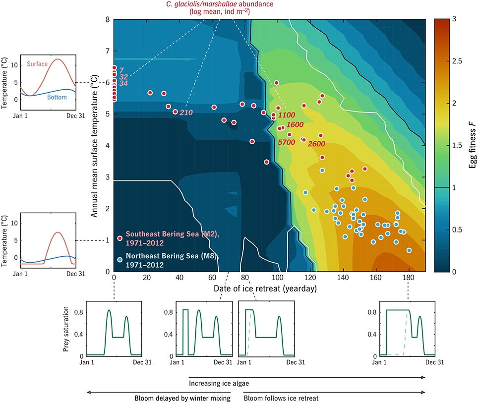
Figure 7. Results of the “Bering” experiment. Color contours give the predicted egg fitness of a C. glacialis/marshallae analog under combinations of ice retreat timing (assumed to control spring bloom timing: Appendix in Supplementary Material) and temperature. Examples of the annual cycles of prey availability P and surface and bottom temperature T₀, T_d are given at left and bottom. Dots locate years 1971–2012 in this timing/temperature parameter space, for the northern (blue) and southern (red) middle shelf. Numbers beside red dots give the measured summer abundance of C. glacialis/marshallae on the southern shelf across years. White contours give the bounds of the central region within which Coltrane predicts one generation per year to be the optimal generation length.

Late summer measurements of C. glacialis/marshallae abundance (individuals m⁻²), averaged over the middle/outer shelf south of 60°N, are shown in Figure 7 for 2003–2010 (n = 364 over the 8 years; Eisner et al., 2014, 2015). Both these observations and the predicted maximum F from Coltrane show a dramatic contrast between the warm years of 2003–05 (t_ice = 0) and the cold years of 2007–2010 (t_ice = 100–130), with the transitional year 2006 harder to interpret. Eisner et al. (2014) found that there was less contrast between cold year/warm year abundance patterns on the northern middle/outer shelf, consistent with the model prediction that all hindcast years on the northern shelf fall within the “viable” habitat range for C. glacialis/marshallae (Figure 7, blue dots).

The viability threshhold that the Southeastern Bering Sea appears to straddle is qualitatively similar to that in the more idealized global experiment (Figures 5, 6), primarily aligned with the phenological index (horizontal axis) rather than the temperature index (vertical axis). The threshhold in the Bering Sea experiment (t_ice ≈ 90–100) falls somewhat beyond the dividing line imposed in the experiment setup between early, ice-retreat-associated blooms and late, open-water blooms (t_ice = 75: see Appendix in Supplementary Material, Sigler et al., 2014). This gap (whose width depends on the mortality level m₀: not shown) indicates that some period of ice algae availability is required by C. glacialis/marshallae in this system, in addition to a favorable pelagic bloom timing.

3.4. Coexisting Life Strategies in Detail: Disko Bay

The experiments above test the ability of Coltrane 1.0 to reproduce first-order patterns in latitude and time but do not provide sensitive tests of the model biology. A model case study in Disko Bay, where populations of three Calanus spp. coexist and have been described in detail (Madsen et al., 2001; Swalethorp et al., 2011), allows a closer examination of the relationships among traits within the family of viable life strategies predicted by Coltrane.

The model forcing (Figure 8) describes a single annual cycle, starting with the 1996 spring bloom. This represents a cold, high-ice state of the system, compared with more recent years in which the spring bloom is earlier (e.g., 2008, Figure 8, Swalethorp et al., 2011) and the deep layer is warmed by Atlantic water intrusions (Hansen et al., 2012). This particular year was chosen because measurements of prey availability and Calanus response by Madsen et al. (2001) were particularly complete and coordinated. A simple attempt to correct the prey field for quality and Calanus preference was made by keeping only the >11 μm size fraction of phytoplankton and adding total microzooplankton, in μg C. The measured phytoplankton C:chl ratio was used to convert the sum to an equivalent chlorophyll concentration, and this time series was then slightly idealized for clarity (Figure 8, Appendix in Supplementary Material).

FIGURE 8

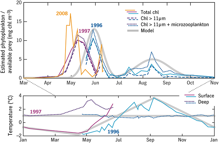
Figure 8. Observations of temperature and prey in Disko Bay 1996–1997 from Madsen et al. (2001) (blue and purple thin lines) used to construct semi-idealized forcing time series for the model (thick gray lines). Three observation-based estimates of the prey field are shown, in each case averaged between the surface and subsurface fluorescence maximum: total chlorophyll (solid), chlorophyll in the >11 μm size fraction (dashed), and >11 μm chlorophyll plus a correction for microzooplankton (dotted). A 2008 time series of total chlorophyll is shown for comparison (orange). Temperature in the upper 50 m (“surface”) and water-column minimum temperature (“deep”) are also shown.

Sensible results were only possible after tuning the predation mortality scale coefficient m₀. It is likely that our simple mortality scheme introduces some form of bias, compared with the reality in this system of predation by successive waves of visual and non-visual predators, which will be considered in a separate study. Still, a sensitivity experiment using the φ model shows that varying m₀ has, as intended, a simple, uniform effect on fitness/population growth (Figure 9) that leaves other trait relationships along the size spectrum unaffected. The φ model predicts that copepods similar to C. finmarchicus in size have much greater fitness at a generation length of 1 year than at 2 years or more; that C. hyperboreus would be unable to complete its life cycle in 1 year, but is well-suited to a 2-year cycle; and that C. glacialis falls in the size range where 1- and 2-year life cycles have comparable fitness value. These results are consistent with observations (Madsen et al., 2001) and more general surveys of life strategies in the three species (Falk-Petersen et al., 2009; Daase et al., 2013).

FIGURE 9

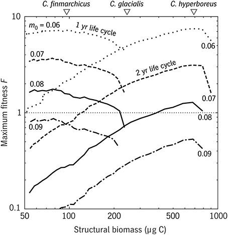
Figure 9. Results of the φ model for a range of u₀ (relative development rate) values in the Disko Bay testbed (Figure 8). Maximum egg fitness F is plotted for 1-year and 2-year strategies, for each of four values of the mortality scaling parameter m₀ (0.06–0.09 d⁻¹), as a function of adult size S. The mean structural weights of the three Calanus spp. that coexist in Disko Bay are also shown (white triangles, top). Curves of F are shown over ranges where survival to adulthood without starvation is possible.

These results naturally raise the question of whether even lower values of u₀—further reductions in development rate—would produce even larger copepods with even longer life cycles in this environment. C. hyperboreus has been reported to have a life cycle of up to 5 years in other systems (Falk-Petersen et al., 2009) and so the question is more than theoretical. In this version of Coltrane, the lower limit on development rate (and thus the upper limit on adult size) are set by the assumption that modulation of this rate is spread uniformly across the developmental period, rather than concentrated in late copepodid stages, as might be more realistic (Campbell et al., 2001). The largest viable adults in the Disko experiment are those that barely reach D = D_s, the start of reserve accumulation, before a first diapause is required.

For greater specificity, we switched from the φ to the ER model version, running a spectrum of t_egg cases (earliest possible egg-production date: see Section 2.5) along with a spectrum of u₀ (development rate) cases. The predicted “community,” then is the set of all combinations of u₀ and t_egg that lead to a viable level of lifetime egg production. An analog for each of the three Calanus spp. is constructed by averaging model results over the set of viable (u₀, t_egg) cases that predict an adult size within 30% of the average measured adult size for that species. The ER model imposes additional constraints on the model organisms—e.g., they are no longer allowed an infinite egg production rate—and to compensate we reduced m₀ from 0.08 d⁻¹ to 0.06 d⁻¹.

The relationship between generation length and adult size across all (u₀, t_egg) combinations is shown in Figure 10. Results are consistent with the φ model (Figure 9) only a 1-year life cycle is viable for C. finmarchicus in this environment, only a 2-year or longer cycle is viable for C. hyperboreus, and C. glacialis again lies near the boundary where the two strategies are comparable. Note that the model allows for a continuum of intermediate cases in the C. finmarchicus–C. glacialis size range, consistent with the observation of hybridization between these species (Parent et al., 2015).

FIGURE 10

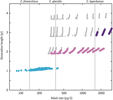
Figure 10. Emergent relationship between generation length and adult size in the Disko Bay model experiment. Large colored dots indicate results for trait combinations that achieve a viable rate of egg production per generation (color coding matches that in Figure 12: blue, generation length of 1 year; light purple, 2 years; dark purple, 3 years) while small gray dots indicate trait combinations that reach maturity without starvation but have egg production rates below replacement level.

The ER model also predicts a time series of egg production associated with each trait combination, which we can compare with observations for each species. The model predicts that C. finmarchicus analogs spawn in close association with the spring bloom, that C. hyperboreus spawns well before the spring bloom, and that C. glacialis is intermediate (Figures 11, 12A). These patterns are all in accordance with Disko Bay observations (Madsen et al., 2001; Swalethorp et al., 2011), although the absolute range is muted: Madsen et al. (2001) report C. hyperboreus spawning as early as February. As one would expect from these timing patterns, the model predicts a significant trend between size and the capital fraction of total egg production E_cap/(E_inc + E_cap) (Figure 12C). Again, the pattern is qualitatively correct but muted: Coltrane predicts 80% income breeding at the size of C. finmarchicus (a pure income breeder in reality) and 80% capital breeding at the size of C. hyperboreus (a pure capital breeder in reality). More notable than the error is how much of the income/capital spectrum can apparently be reproduced as a consequence of optimizing reproductive timing alone Varpe et al. (2009), without imposing the physiological difference between the two strategies as an independent trait (Ejsmond et al., 2015).

FIGURE 11

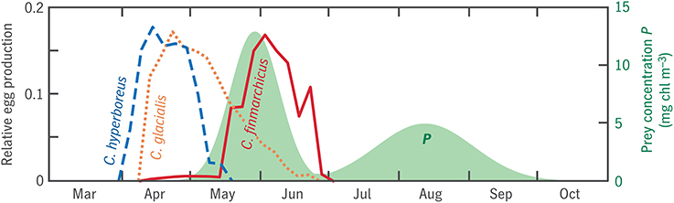
Figure 11. Seasonal progression of egg production in model analogs for three Calanus spp. in Disko Bay (lines), in relation to prey concentration P (shaded). Egg production time series consist of n(t₀), the first eigenvector of the transition matrix V discussed in Section 2.4.3, normalized to integrate to 1.

FIGURE 12

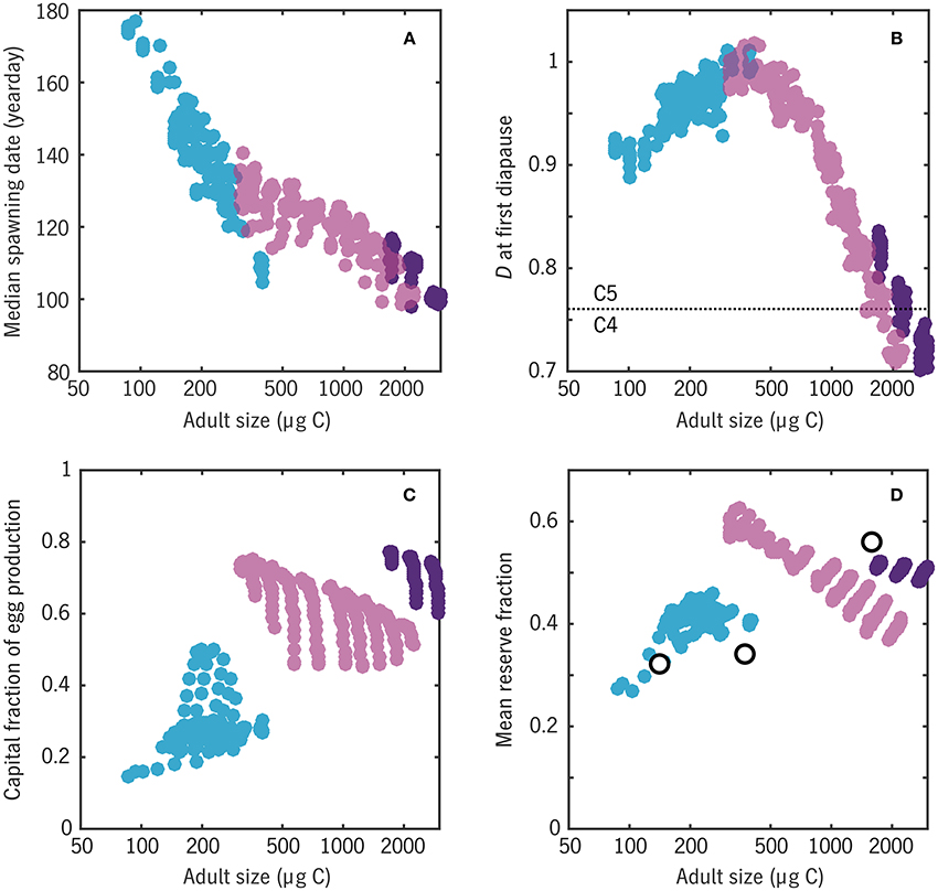
Figure 12. Relationships between a number of emergent traits with adult body size in the Disko Bay experiment. Color coding matches Figure 10, distinguishing 1-year (blue), 2-year (light purple), and 3-year (dark purple) life cycles. (A) Median spawning date: cf. peaks of egg production curves in Figure 11. (B) Earliest developmental stage D at which diapause (a = 0) occurs: values have been jittered slightly in the vertical for clarity. (C) Capital fraction of egg production E_cap/(E_inc + Ecap). (D) Mean reserve fraction of individual biomass R/(R + S), compared with wax esters as a fration of total body carbon for three Calanus spp. from Swalethorp et al. (2011) (open circles).

The model predicts (Figure 12B) that the largest model organisms, with the longest generation lengths, enter their first diapause near the boundary between copepodite stages C4 and C5 (D ≈ 0.75), whereas smaller organisms enter first diapause well into stage C5. Madsen et al. (2001) found that both C. glacialis and C. hyperboreus diapause as C4, C5, and adults in Disko Bay, suggesting that the model is biased toward fast maturation. The discrepancy could also be related to intraspecific variation in the real populations or non-equiproportional development in the late stages, i.e., a variable conversion scale between actual developmental stage and D.

Finally, the ER version of Coltrane allows an estimate of the fraction of individual carbon in the form of storage lipids R/(R + S) (Figure 12D). Averaging each model population from the first diapause-capable stage D = D_dia through adulthood, weighted by survivorship N, yields an overall range that compares well with the species-mean wax ester fractions measured by Swalethorp et al. (2011): ~30% for C. finmarchicus to ~60% for C. hyperboreus. In the middle of the size spectrum, reserve fraction is highly variable across viable 2-year strategies, a warning that the success of this final model prediction may be partly fortuitous. Still, taken as a whole, this experiment has yielded a striking result: that a small set of energetic and timing contraints is able to correctly predict, a priori, that Disko Bay should be able to support a spectrum of calanoid copepods from income breeders with an adult size ~100 μg C, a 1-year life cycle, and a wax ester fraction ~30% to capital breeders with an adult size ~1000 μg C, a two-or-more-year life cycle, and a wax ester fraction ~60%.

4. Discussion

4.1. Temperature and Timing

In the results above, whether prey availability is treated simply (Figures 5, 6) or with site-specific detail (Figure 7), it appears that the viability of the calanoid community near its high-latitude limit is more sensitive to prey abundance and phenology than to temperature. This result is heuristically similar to the conclusions of Ji et al. (2012) and Feng et al. (2016), although the exact physiological mechanisms differ. Alcaraz et al. (2014) suggested based on lab experiments that C. glacialis reaches an bioenergetic limit near 6°C, and Holding et al. (2013) and others have hypothesized that thermal limits will produce ecosystem-level tipping points in the warming Arctic. Our results, in contrast, suggest that thermal tipping points, even if present at the population level, do not generalize to the community level in copepods. Rather, the model predicts complete continuity between the life strategy of Arctic C. glacialis and temperate congeners like C. marshallae (Figure 6). It also suggests that even on the population level in the Bering Sea, warm/cold-year variation in prey availability is a sufficient explanation of variability in the abundance of C. glacialis/marshallae (Figure 7), without the invocation of a thermal threshhold.

Both the global and Bering experiments suggest, furthermore, that increasing water temperature per se is not necessarily a stressor on copepod communities, even high-latitude communities. In both cases, the low-prey viability threshhold actually relaxes (i.e., is tilted toward lower prey values) as temperature increases, indicating that in these testbeds, the positive effect of temperature on growth and maturation rate actually outweighs the effect of temperature on metabolic losses and overwinter survival (This result may be reliant on the model assumption that the stage of first diapause is highly plastic). In cases where deep, overwintering temperatures increase faster than surface temperatures (Hansen et al., 2012) this balance may not hold, and in the real ocean changes in temperature are highly confounded with changes in phytoplankton production and phenology. Still, it is notable that the model predicts that warming temperatures will have a non-monotonic effect on copepod populations (∂F/∂T₀ ≷ 0, Figures 5, 6) even when metabolic thermal threshholds sensu Alcaraz et al. (2014) and changes in prey availability are not considered. These results are a caution against overly simple climate-impacts projections based on temperature alone.

4.2. Uncertainties and Unresolved Processes

The biology in Coltrane could be refined in many ways, but two issues stand out as being both mechanistically uncertain and sensitive controls on model behavior. These correspond to the two parameters that it was necessary to tune among model experiments (Table 2) the obstacles to formulation of a fully portable scheme that could produce accurate results across the full range of environments considered here with a single parameterization.

The first of these is the perennial problem of the mortality closure. We modeled predation mortality as size-dependent according to the same power law used for ingestion and metabolism, a choice which is mathematically convenient and makes the effect of top-down controls, if not minor, then at least simple and easy to detect (Figure 9). This size scaling is consistent with the review by Hirst and Kiørboe (2002) but that study also shows that the variation in copepod mortality not explained by allometry spans orders of magnitude (cf. Ohman et al., 2004). Indeed, in some cases one might posit exactly the opposite pattern, in which mortality due to visual predators like larval fish increases with prey body size (Fiksen et al., 1998; Varpe et al., 2015). This latter pattern is one hypothesis for why in reality C. hyperboreus is confined to high latitudes, whereas the model predicts no southern (warm, high-prey) habitat limit to C. hyperboreus analogs based on bottom-up considerations (Figure 5). Merging Coltrane 1.0 with a light- and size-based predation scheme similar to Varpe et al. (2015) or Ohman and Romagnan (2015) would allow one to better test the balance of bottom-up and top-down controls on calanoid biogeography.

Second, our experience constructing the Bering Sea and Disko Bay cases suggests that the greatest uncertainty in the model bioenergetics is actually not the physiology itself—empirical reviews like Saiz and Calbet (2007), Maps et al. (2014), Kiørboe and Hirst (2014), and Banas and Campbell (2016) have constrained the key rates moderately well—but rather the problem of translating a prey field into a rate of ingestion. Within each of our model testbeds, the prey time series P remains subject to uncertainty in relative grazing rates on ice algae, large and small pelagic phytoplankton, and microzooplankton, despite a wealth of local observations and a history of work on this problem in Calanus specifically (Olson et al., 2006; Campbell et al., 2009, in press). The precision of each testbed, and even moreso the ambition of generalizing across them, is also limited by uncertainty in the shape of the functional response (Frost, 1980; Gentleman et al., 2003), here represented by a half-saturation coefficient, which has not been found to be consistent across site-specific studies (Campbell et al., in press; Møller et al., 2016) or well-constrained by general reviews (Hansen et al., 1997). This ambiguity is perhaps not surprising when one considers that ingestion as a function of chlorophyll or prey carbon is not a simple biomechanical property, but in fact a plastic behavioral choice. Accordingly, it might well be responsive not only to mean or maximum prey concentration but also to the prey distribution over the water column, the tradeoff between energy gain and predation risk (Visser and Fiksen, 2013), prey composition and nutritional value, and the context of the annual routine. These issues are fundamental to concretely modeling the effect of microplankton dynamics on mesozooplankton grazers. Addressing them systematically in models will require novel integration between what could be called oceanographic and marine-biological perspectives on large zooplankton.

5. Conclusion

Coltrane 1.0, introduced here, is a minimalist model of copepod life history and population dynamics, a metacommunity-level framework on which additional species- or population-level constraints can be layered. Many present and future patterns in large copepods might well prove to be sensitive to species-specific constraints that Coltrane 1.0 does not resolve, such as thermal adaptation, physiological requirements for egg production, or cues for diapause entry and exit. Nevertheless, the model experiments above demonstrate that many patterns in latitude, time, and trait space can be replicated numerically even when we only consider a few key constraints on the individual energy budget: the total energy available in a given environment per year; the energy and time required to build an adult body; the metabolic and predation penalties for taking too long to reproduce; and the size and temperature dependence of the vital rates involved.

Results of the global and Bering experiments (Figures 5–7) suggest that timing and seasonality are crucial to large copepods, but not because of match/mismatch (Edwards and Richardson, 2004) the model organisms are free to resolve timing mismatches with complete plasticity. Rather, these results highlight the role of seasonality in the sense of total energy available for growth and development per year, or the number of weeks per year of net energy gain relative to the number of weeks of net deficit. The simplicity of this view means that the model scheme and results may generalize far beyond copepods with only minor modification.

The exercise of parameterizing the Bering Sea and Disko Bay cases, and of attempting to map real environments onto an idealized parameter space in the global experiment (Figure 6), highlighted that the real limit on our ability to predict the fate of copepods in changing oceans may not be our incomplete knowledge of their physiology, but rather our incomplete knowledge of how their environments appear from their point of view. How do standard oceanographic measures of chlorophyll and particulate chemistry relate to prey quality, and how much risk a copepod should take on in order to forage in the euphotic zone? How do bathymetry, the light field, and other metrics relate to the predator regime? Further experiments in a simple, fast, mechanistically transparent model like Coltrane may suggest new priorities for field observations, in addition to new approaches to regional and global modeling.

Author Contributions

NB designed the model, performed the analysis, and led the writing of the manuscript. EM and TN helped formulate and interpret the Disko Bay case study, and LE the Bering Sea case study. All authors contributed to revision of the manuscript.

Funding

This work was supported by grants PLR-1417365 and PLR-1417224 from the National Science Foundation.

Conflict of Interest Statement

The authors declare that the research was conducted in the absence of any commercial or financial relationships that could be construed as a potential conflict of interest.

The reviewer ØF and handling Editor declared their shared affiliation, and the handling Editor states that the process nevertheless met the standards of a fair and objective review.

Acknowledgments

Many thanks to Bob Campbell, Thomas Kiørboe, Øystein Varpe, Dougie Speirs, and Aidan Hunter for discussions that helped shape both the model and the questions we asked of it. Thanks as well to Nick Record, Carin Ashjian, and ØF, whose comments much improved the manuscript.

Supplementary Material

The Supplementary Material for this article can be found online at: https://www.frontiersin.org/article/10.3389/fmars.2016.00225/full#supplementary-material

References

Alcaraz, M., Felipe, J., Grote, U., Arashkevich, E., and Nikishina, A. (2014). Life in a warming ocean: thermal thresholds and metabolic balance of arctic zooplankton. J. Plankton Res. 36, 3–10. doi: 10.1093/plankt/fbt111

CrossRef Full Text | Google Scholar

Ashjian, C. J., Campbell, R. G., Welch, H. E., Butler, M., and Van Keuren, D. (2003). Annual cycle in abundance, distribution, and size in relation to hydrography of important copepod species in the western Arctic Ocean. Deep Sea Res. Part I 50, 1235–1261. doi: 10.1016/S0967-0637(03)00129-8

CrossRef Full Text | Google Scholar

Banas, N. S. Campbell, R. G. (2016). Traits controlling body size in copepods: separating general constraints from species-specific strategies. Mar. Ecol. Prog. Ser. 558, 21–33. doi: 10.3354/meps11873

CrossRef Full Text | Google Scholar

Banas, N. S., Zhang, J., Campbell, R. G., Sambrotto, R. N., Lomas, M. W., Sherr, E., et al. (2016). Spring plankton dynamics in the Eastern Bering Sea, 1971-2050: mechanisms of interannual variability diagnosed with a numerical model. J. Geophys. Res. 121, 1476–1501. doi: 10.1002/2015jc011449

CrossRef Full Text | Google Scholar

Barton, A. D., Pershing, A. J., Litchman, E., Record, N. R., Edwards, K. F., Finkel, Z. V., et al. (2013). The biogeography of marine plankton traits. Ecol. Lett. 16, 522–534. doi: 10.1111/ele.12063

PubMed Abstract | CrossRef Full Text | Google Scholar

Beaugrand, G. Kirby, R. R. (2010). Climate, plankton and cod. Glob. Change Biol. 16, 1268–1280. doi: 10.1111/j.1365-2486.2009.02063.x

CrossRef Full Text | Google Scholar

Burke, B. J., Peterson, W. T., Beckman, B. R., Morgan, C., Daly, E. A., and Litz, M. (2013). Multivariate models of adult pacific salmon returns. PLoS ONE 8:e54134. doi: 10.1371/journal.pone.0054134

PubMed Abstract | CrossRef Full Text | Google Scholar

Campbell, R. G., Ashjian, C. J., Sherr, E. B., Sherr, B. F., Lomas, M. W., Ross, C., et al. (in press). Mesozooplankton grazing during spring sea-ice conditions in the eastern Bering Sea. Deep Sea Res. Part II. doi: 10.1016/j.dsr2.2015.11.003

CrossRef Full Text | Google Scholar

Campbell, R. G., Sherr, E. B., Ashjian, C. J., Plourde, S., Sherr, B. F., Hill, V., et al. (2009). Mesozooplankton prey preference and grazing impact in the western Arctic Ocean. Deep Sea Res. Part II 56, 1274–1289. doi: 10.1016/j.dsr2.2008.10.027

CrossRef Full Text | Google Scholar

Campbell, R. G., Wagner, M. M., Teegarden, G. J., Boudreau, C. A., and Durbin, E. G. (2001). Growth and development rates of the copepod Calanus finmarchicus reared in the laboratory. Mar. Ecol. Prog. Ser. 221, 161–183. doi: 10.3354/meps221161

CrossRef Full Text | Google Scholar

Chesson, P. (2000). Mechanisms of maintenance of species diversity. Annu. Rev. Ecol. Syst. 31, 343–366. doi: 10.1146/annurev.ecolsys.31.1.343

CrossRef Full Text | Google Scholar

Clark, J. R., Lenton, T. M., Williams, H. T. P., and Daines, S. J. (2013). Environmental selection and resource allocation determine spatial patterns in picophytoplankton cell size. Limnol. Oceanogr. 58, 1008–1022. doi: 10.4319/lo.2013.58.3.1008

CrossRef Full Text | Google Scholar

Cooper, L. W., Sexson, M. G., Grebmeier, J. M., Gradinger, R., Mordy, C. W., and Lovvorn, J. R. (2013). Linkages between sea-ice coverage, pelagic-benthic coupling, and the distribution of spectacled eiders: observations in March 2008, 2009 and 2010, northern Bering Sea. Deep Sea Res. 94, 31–43. doi: 10.1016/j.dsr2.2013.03.009

CrossRef Full Text | Google Scholar

Coyle, K. O., Eisner, L. B., Mueter, F. J., Pinchuk, A. I., Janout, M. A., Cieciel, K. D., et al. (2011). Climate change in the southeastern Bering Sea: impacts on pollock stocks and implications for the oscillating control hypothesis. Fish. Oceanogr. 20, 139–156. doi: 10.1111/j.1365-2419.2011.00574.x

CrossRef Full Text | Google Scholar

Daase, M., Falk-Petersen, S., Varpe, Ø., Darnis, G., Søreide, J. E., Wold, A., et al. (2013). Timing of reproductive events in the marine copepod Calanus glacialis: a pan-Arctic perspective. Can. J. Fish. Aquat. Sci. 70, 871–884. doi: 10.1139/cjfas-2012-0401

CrossRef Full Text | Google Scholar

Durbin, E. G. Casas, M. C. (2014). Early reproduction by Calanus glacialis in the Northern Bering Sea: the role of ice algae as revealed by molecular analysis. J. Plankton Res. 36, 523–541. doi: 10.1093/plankt/fbt121

CrossRef Full Text | Google Scholar

Edwards, M. Richardson, A. J. (2004). Impact of climate change on marine pelagic phenology and trophic mismatch. Nature 430, 881–884. doi: 10.1038/nature02808

PubMed Abstract | CrossRef Full Text | Google Scholar

Eisner, L. B., Napp, J. M., Mier, K. L., Pinchuk, A. I., and Andrews, A. G. (2014). Climate-mediated changes in zooplankton community structure for the eastern Bering Sea. Deep Sea Res. Part II 109, 157–171. doi: 10.1016/j.dsr2.2014.03.004

CrossRef Full Text | Google Scholar

Eisner, L. B., Siddon, E. C., and Strasburger, W. W. (2015). Spatial and temporal changes in assemblage structure of zooplankton and pelagic fish in the eastern Bering Sea across varying climate conditions. Izvestia TINRO 181, 141–160. Available online at: http://cyberleninka.ru/article/n/spatial-and-temporal-changes-in-assemblage-structure-of-zooplankton-and-pelagic-fish-in-the-eastern-bering-sea-across-varying-climate

Ejsmond, M. J., Varpe, Ø., Czarnoleski, M., and Kozłowski, J. (2015). Seasonality in offspring value and trade-offs with growth explain capital breeding. Am. Nat. 186, E111–E125. doi: 10.1086/683119

CrossRef Full Text | Google Scholar

Falk-Petersen, S., Mayzaud, P., Kattner, G., and Sargent, J. R. (2009). Lipids and life strategy of Arctic Calanus. Mar. Biol. Res. 5, 18–39. doi: 10.1080/17451000802512267

CrossRef Full Text | Google Scholar

Feng, Z., Ji, R., Campbell, R. G., Ashjian, C. J., and Zhang, J. (2016). Early ice retreat and ocean warming may induce copepod biogeographic boundary shifts in the Arctic Ocean. J. Geophys. Res. 121, 6137–6158. doi: 10.1002/2016JC011784

CrossRef Full Text | Google Scholar

Fiksen, Ø., Utne, A. C. W., Aksnes, D. L., Eiane, K., Helvik, J. V., and Sundby, S. (1998). Modeling the influence of light, turbulence and ontogeny on ingestion rates in larval cod and herring. Fish. Oceanogr. 7, 355–363. doi: 10.1046/j.1365-2419.1998.00068.x

CrossRef Full Text | Google Scholar

Forster, J., Hirst, A. G., and Woodward, G. (2011). Growth and development rates have different thermal responses. Am. Nat. 178, 668–678. doi: 10.1086/662174

PubMed Abstract | CrossRef Full Text | Google Scholar

Frost, B. W. (1980). “The inadequacy of body size as an indicator of niches in the zooplankton,” in Evolution and Ecology of Zooplankton Communities, ed W. C. Kerfoot (Hanover, NH: University Press), 742–753.

Gentleman, W., Leising, A. W., Frost, B. W., Strom, S. L., and Murray, J. (2003). Functional responses for zooplankton feeding on multiple resources: a review of assumptions and biological dynamics. Deep Sea Res. Part II 50, 2847–2875. doi: 10.1016/j.dsr2.2003.07.001

CrossRef Full Text | Google Scholar

Gurney, W. S. C., Crowley, P. H., and Nisbet, R. M. (1992). Locking life-cycles onto seasons: circle-map models of population dynamics and local adaptation. J. Math. Biol. 30, 251–279. doi: 10.1007/BF00176151

CrossRef Full Text | Google Scholar

Hansen, J., Bjornsen, P. K., and Hansen, B. W. (1997). Zooplankton grazing and growth: scaling within the 2-2,000 μm body size range. Limnol. Oceanogr. 42, 687–704. doi: 10.4319/lo.1997.42.4.0687

CrossRef Full Text | Google Scholar

Hansen, M. O., Nielsen, T. G., Stedmon, C. A., and Munk, P. (2012). Oceanographic regime shift during 1997 in Disko Bay, Western Greenland. Limnol. Oceanogr. 57, 634–644. doi: 10.4319/lo.2012.57.2.0634

CrossRef Full Text | Google Scholar

Heath, M., Boyle, P., Gislason, A., Gurney, W., Hay, S. J., Head, E. J. H., et al. (2004). Comparative ecology of over-wintering Calanus finmarchicus in the northern North Atlantic, and implications for life-cycle patterns. ICES J. Mar. Sci. 61, 698–708. doi: 10.1016/j.icesjms.2004.03.013

CrossRef Full Text | Google Scholar

Hirche, H.-J. Kattner, G. (1993). Egg production and lipid content of Calanus glacialis in spring: indication of a food-dependent and food-independent reproductive mode. Mar. Biol. 117, 615–622. doi: 10.1007/BF00349773

CrossRef Full Text | Google Scholar

Hirst, A. G. Kiørboe, T. (2002). Mortality of marine planktonic copepods: global rates and patterns. Mar. Ecol. Prog. Ser. 230, 195–209. doi: 10.3354/meps230195

CrossRef Full Text | Google Scholar

Holding, J. M., Duarte, C. M., and Arrieta, J. M. (2013). Experimentally determined temperature thresholds for Arctic plankton community metabolism. Biogeosciences 10, 357–370. doi: 10.5194/bg-10-357-2013

CrossRef Full Text | Google Scholar

Holt, R. D., Grover, J., and Tilman, D. (1994). Simple rules for interspecific dominance in systems with exploitative and apparent competition. Am. Nat. 144, 741–771. doi: 10.1086/285705

CrossRef Full Text | Google Scholar

Hooff, R. C. Peterson, W. (2006). Copepod biodiversity as an indicator of changes in ocean and climate conditions of the northern California current ecosystem. Limnol. Oceanogr. 51, 2607–2620. doi: 10.4319/lo.2006.51.6.2607

CrossRef Full Text | Google Scholar

Houston, A. I., McNamara, J. M., and Hutchinson, J. M. C. (1993). General results concerning the trade-off between gaining energy and avoiding predation. Philos. Trans. Roy. Soc. Lond. B 341, 375–397. doi: 10.1098/rstb.1993.0123

CrossRef Full Text | Google Scholar

Hunt, G. L., Coyle, K. O., Eisner, L. B., Farley, E. V., Heintz, R. A., Mueter, F. J., et al. (2011). Climate impacts on eastern Bering Sea foodwebs: a synthesis of new data and an assessment of the Oscillating Control Hypothesis. ICES J. Mar. Sci. 68, 1230–1243. doi: 10.1093/icesjms/fsr036

CrossRef Full Text | Google Scholar

Hunt, G. L., Stabeno, P. J., Walters, G., Sinclair, E., Brodeur, R. D., Napp, J. M., et al. (2002). Climate change and control of the southeastern Bering Sea pelagic ecosystem. Deep Sea Res. 49, 5821–5853. doi: 10.1016/s0967-0645(02)00321-1

CrossRef Full Text | Google Scholar

Ji, R., Ashjian, C. J., Campbell, R. G., Chen, C., Gao, G., Davis, C., et al. (2012). Life history and biogeography of Calanus copepods in the Arctic Ocean: an individual-based modeling study. Prog. Oceanogr. 96, 40–56. doi: 10.1016/j.pocean.2011.10.001

CrossRef Full Text | Google Scholar

Kattner, G. Hagen, W. (2009). “Lipids in marine copepods: latitudinal characteristics and perspective to global warming,” in Lipids in Aquatic Ecosystems, ed M. T. Arts (New York, NY: Springer), 257–280.

Kiørboe, T. Hirst, A. G. (2014). Shifts in mass scaling of respiration, feeding, and growth rates across life-form transitions in marine pelagic organisms. Am. Nat. 183, E118–E130. doi: 10.1086/675241

PubMed Abstract | CrossRef Full Text | Google Scholar

Kiørboe, T. Sabatini, M. (1995). Scaling of fecundity, growth and development in marine planktonic copepods. Mar. Ecol. Prog. Ser. 120, 285–298. doi: 10.3354/meps120285

CrossRef Full Text | Google Scholar

Kleiber, M. (1932). Body size and metabolism. Hilgardia 6, 315–353. doi: 10.3733/hilg.v06n11p315

CrossRef Full Text

Maar, M., Møller, E. F., Gürkan, Z., Jónasdóttir, S. H., and Nielsen, T. G. (2013). Sensitivity of Calanus spp. copepods to environmental changes in the North Sea using life-stage structured models. Prog. Oceanogr. 111, 24–37. doi: 10.1016/j.pocean.2012.10.004

CrossRef Full Text | Google Scholar

MacDonald, A., Heath, M., Edwards, M., Furness, R., Pinnegar, J., Wanless, S., et al. (2015). “Climate-driven trophic cascades affecting seabirds around the British Isles,” in Oceanography and Marine Biology, eds R. N. Hughes, D. J. Hughes, I. P. Smith, and A. C. Dale (Oxford: CRC Press), 55–80.

Mackas, D. L., Greve, W., Edwards, M., Chiba, S., Tadokoro, K., Eloire, D., et al. (2012). Changing zooplankton seasonality in a changing ocean: comparing time series of zooplankton phenology. Prog. Oceanogr. 97–100, 31–62. doi: 10.1016/j.pocean.2011.11.005

CrossRef Full Text | Google Scholar

Madsen, S. D., Hansen, B. W., and Nielsen, T. G. (2001). Annual population development and production by Calanus finmarchicus, C. glacialis and C. hyperboreus in Disko Bay, western Greenland. Mar. Biol. 139, 75–83. doi: 10.1007/s002270100552

CrossRef Full Text | Google Scholar

Mantua, N. J., Hare, S. R., Zhang, Y., Wallace, J. M., and Francis, R. C. (1997). A Pacific interdecadal climate oscillation with impacts on salmon production. Bull. Am. Meteorol. Soc. 78, 1069–1079. doi: 10.1175/1520-0477(1997)078<1069:APICOW>2.0.CO;2

CrossRef Full Text | Google Scholar

Maps, F., Pershing, A. J., and Record, N. R. (2012). A generalized approach for simulating growth and development in diverse marine copepod species. ICES J. Mar. Sci. 69, 370–379. doi: 10.1093/icesjms/fsr182

CrossRef Full Text | Google Scholar

Maps, F., Record, N. R., and Pershing, A. J. (2014). A metabolic approach to dormancy in pelagic copepods helps explaining inter- and intra-specific variability in life-history strategies. J. Plankton Res. 36, 18–30. doi: 10.1093/plankt/fbt100

CrossRef Full Text | Google Scholar

Miller, C. B., Lynch, D. R., Carlotti, F., Gentleman, W., and Lewis, C. V. W. (2002). Coupling of an individual-based population dynamic model of Calanus finmarchicus to a circulation model for the Georges Bank region. Fish. Oceanogr. 7, 219–234. doi: 10.1046/j.1365-2419.1998.00072.x

CrossRef Full Text | Google Scholar

Møller, E. F., Bohr, M., Kjellerup, S., Maar, M., Mohl, M., Swalethorp, R., et al. (2016). Calanus finmarchicus egg production at its northern border. J. Plankton Res. 38, 1206–1214. doi: 10.1093/plankt/fbw048

CrossRef Full Text | Google Scholar

Møller, E. F., Maar, M., Jónasdóttir, S. H., Gissel Nielsen, T., and Tönnesson, K. (2012). The effect of changes in temperature and food on the development of Calanus finmarchicus and Calanus helgolandicus populations. Limnol. Oceanogr. 57, 211–220. doi: 10.4319/lo.2012.57.1.0211

CrossRef Full Text | Google Scholar

Ohman, M. D., Eiane, K., Durbin, E., Runge, J., and Hirche, H.-J. (2004). A comparative study of Calanus finmarchicus mortality patterns at five localities in the North Atlantic. ICES J. Mar. Sci. 61, 687–697. doi: 10.1016/j.icesjms.2004.03.016

CrossRef Full Text | Google Scholar

Ohman, M. D. Romagnan, J.-B. (2015). Nonlinear effects of body size and optical attenuation on Diel vertical migration by zooplankton. Limnol. Oceanogr. 61, 765–770. doi: 10.1002/lno.10251

CrossRef Full Text

Olson, M. B., Lessard, E. J., and Wong, C. (2006). Copepod feeding selectivity on microplankton, including the toxigenic diatoms Pseudo-nitzschia spp., in the coastal Pacific Northwest. Mar. Ecol. Prog. Ser. 326, 207–220. doi: 10.3354/meps326207

CrossRef Full Text | Google Scholar

Österblom, H., Olsson, O., Blenckner, T., and Furness, R. W. (2008). Junk-food in marine ecosystems. Oikos 117, 967–977. doi: 10.1111/j.0030-1299.2008.16501.x

CrossRef Full Text | Google Scholar

Parent, G. J., Plourde, S., Joly, P., and Turgeon, J. (2015). Phenology and fitness of Calanus glacialis, C. finmarchicus (Copepoda), and their hybrids in the St. Lawrence Estuary. Mar. Ecol. Prog. Ser. 524, 1–9. doi: 10.3354/meps11240

CrossRef Full Text | Google Scholar

Peterson, W. T. (1979). Life History and Ecology of Calanus marshallae Frost in the Oregon Upwelling Zone. Ph.D. thesis, Oregon State University.

Peterson, W. T. (1986). Development, growth, and survivorship of the copepod Calanus marshallae in the laboratory. Mar. Ecol. Prog. Ser. 29, 61–72. doi: 10.3354/meps029061

CrossRef Full Text

Record, N. R., Pershing, A. J., and Maps, F. (2012). First principles of copepod development help explain global marine diversity patterns. Oecologia 170, 289–295. doi: 10.1007/s00442-012-2313-0

PubMed Abstract | CrossRef Full Text | Google Scholar

Record, N. R., Pershing, A. J., and Maps, F. (2013). Emergent copepod communities in an adaptive trait-structured model. Ecol. Model. 260, 11–24. doi: 10.1016/j.ecolmodel.2013.03.018

CrossRef Full Text | Google Scholar

Record, N. R., Pershing, A. J., and Maps, F. (2014). The paradox of the “paradox of the plankton.” ICES J. Mar. Sci. 71, 236–240. doi: 10.1093/icesjms/fst049

CrossRef Full Text | Google Scholar

Rey-Rassat, C., Irigoien, X., Harris, R., Head, R., and Carlotti, F. (2002). Growth and development of Calanus helgolandicus reared in the laboratory. Mar. Ecol. Prog. Ser. 238, 125–138. doi: 10.3354/meps238125

CrossRef Full Text | Google Scholar

Runge, J. A., Plourde, S., Joly, P., Niehoff, B., and Durbin, E. (2006). Characteristics of egg production of the planktonic copepod, Calanus finmarchicus, on Georges Bank: 1994–1999. Deep Sea Res. Part II 53, 2618–2631. doi: 10.1016/j.dsr2.2006.08.010

CrossRef Full Text | Google Scholar

Sainmont, J., Andersen, K. H., Thygesen, U. H., Fiksen, Ø., and Visser, A. W. (2015). An effective algorithm for approximating adaptive behavior in seasonal environments. Ecol. Model. 311, 20–30. doi: 10.1016/j.ecolmodel.2015.04.016

CrossRef Full Text | Google Scholar

Saiz, E. Calbet, A. (2007). Scaling of feeding in marine calanoid copepods. Limnol. Oceanogr. 52, 668–675. doi: 10.4319/lo.2007.52.2.0668

CrossRef Full Text | Google Scholar

Sigler, M. F., Stabeno, P. J., Eisner, L. B., Napp, J. M., and Mueter, F. J. (2014). Spring and fall phytoplankton blooms in a productive subarctic ecosystem, the eastern Bering Sea, during 1995–2011. Deep Sea Res. Part II 109, 71–83. doi: 10.1016/j.dsr2.2013.12.007

CrossRef Full Text | Google Scholar

Stabeno, P. J., Farley, E. V. Jr., Kachel, N. B., Moore, S., Mordy, C. W., Napp, J. M., et al. (2012a). A comparison of the physics of the northern and southern shelves of the eastern Bering Sea and some implications for the ecosystem. Deep Sea Res. Part II 65–70, 14–30. doi: 10.1016/j.dsr2.2012.02.019

CrossRef Full Text | Google Scholar

Stabeno, P. J., Kachel, N. B., Moore, S., Napp, J. M., Sigler, M. F., Yamaguchi, A., et al. (2012b). Comparison of warm and cold years on the southeastern Bering Sea shelf and some implications for the ecosystem. Deep Sea Res. Part II 65–70, 31–45. doi: 10.1016/j.dsr2.2012.02.020

CrossRef Full Text | Google Scholar

Swalethorp, R., Kjellerup, S., Dünweber, M., Nielsen, T. G., Møller, E. F., Rysgaard, S., et al. (2011). Grazing, egg production, and biochemical evidence of differences in the life strategies of Calanus finmarchicus, C. glacialis and C. hyperboreus in Disko Bay, western Greenland. Mar. Ecol. Prog. Ser. 429, 125–144. doi: 10.3354/meps09065

CrossRef Full Text | Google Scholar

Varpe, Ø., Daase, M., and Kristiansen, T. (2015). A fish-eye view on the new Arctic lightscape. ICES J. Mar. Sci. 72, 2532–2538. doi: 10.1093/icesjms/fsv129

CrossRef Full Text | Google Scholar

Varpe, Ø., Jørgensen, C., Tarling, G. A., and Fiksen, Ø. (2007). Early is better: seasonal egg fitness and timing of reproduction in a zooplankton life-history model. Oikos 116, 1331–1342. doi: 10.1111/j.0030-1299.2007.15893.x

CrossRef Full Text | Google Scholar

Varpe, Ø., Jørgensen, C., Tarling, G. A., and Fiksen, Ø. (2009). The adaptive value of energy storage and capital breeding in seasonal environments. Oikos 118, 363–370. doi: 10.1111/j.1600-0706.2008.17036.x

CrossRef Full Text | Google Scholar

Visser, A. W. Fiksen, Ø. (2013). Optimal foraging in marine ecosystem models: selectivity, profitability and switching. Mar. Ecol. Prog. Ser. 473, 91–101. doi: 10.3354/meps10079

CrossRef Full Text | Google Scholar

Visser, A. W., Mariani, P., and Pigolotti, S. (2008). Swimming in turbulence: zooplankton fitness in terms of foraging efficiency and predation risk. J. Plankton Res. 31, 121–133. doi: 10.1093/plankt/fbn109

CrossRef Full Text | Google Scholar

Wilson, R. J., Heath, M. R., and Speirs, D. C. (2016). Spatial modeling of Calanus finmarchicus and Calanus helgolandicus: parameter differences explain differences in biogeography. Front. Mar. Sci. 3:157. doi: 10.3389/fmars.2016.00157

CrossRef Full Text | Google Scholar

Wilson, R. J., Speirs, D. C., and Heath, M. R. (2015). On the surprising lack of differences between two congeneric calanoid copepod species, Calanus finmarchicus and C. helgolandicus. Prog. Oceanogr. 134, 413–431. doi: 10.1016/j.pocean.2014.12.008

CrossRef Full Text | Google Scholar

Zhang, J., Woodgate, R., and Mangiameli, S. (2012). Towards seasonal prediction of the distribution and extent of cold bottom waters on the Bering Sea shelf. Deep Sea Res. Part II 65, 58–71. doi: 10.1016/j.dsr2.2012.02.023

CrossRef Full Text | Google Scholar

Zhang, J., Woodgate, R., and Moritz, R. (2010). Sea ice response to atmospheric and oceanic forcing in the Bering Sea. J. Phys. Oceanogr. 40, 1729–1747. doi: 10.1175/2010JPO4323.1

CrossRef Full Text | Google Scholar