A Model Simulation of the Adaptive Evolution through Mutation of the Coccolithophore Emiliania huxleyi Based on a Published Laboratory Study

Introduction

The climate has been changing and is expected to continue to change—and possibly at an increasing rate (Collins et al., 2013; Rhein et al., 2013) The oceans are intimately involved in both regulating and responding to that change, and marine ecosystems are and will continue to change in response to changes associated with a changing climate (Hoegh-Guldberg et al., 2014; Pörtner et al., 2014; Wong et al., 2014). However, coupled climate-ecosystem models that predict future changes in marine ecosystems, for the most part use fixed compartment model structures for ecosystems with minimally-adaptive parameters: mainly variable C:N ratios and a temperature dependence of some intrinsic rates such as phytoplankton growth rate (e.g., Chust et al., 2014). While we use these models to predict the future structure and function of marine ecosystems, considerable skepticism remains (e.g., Planque, 2015).

Increasing temperature is the first order environmental change affecting marine species. In response, the ranges of most species are shifting poleward, nearly 2° latitude per decade, ~190 km ± 20%(SE) (e.g., Sorte et al., 2010). In particular, Emiliania huxleyi blooms in polar regions became more frequent and of greater extent in SeaWiFS satellite imagery (1997-2007) compared with CZCS imagery (1978-1986) (Winter et al., 2014). The large variability in rates of poleward shift for different species means, for example, that the species assemblage (of fishes) in a fixed region is changing (Simpson et al., 2011). Other documented changes in response to warming are in phenology: for example, open ocean and coastal zooplankton reaching their biomass maximum ~1 month earlier over 40 years, correlated with the total number of “degree-days” above 6°C over the spring months of March-April-May (Mackas et al., 2007).

There are three other main mechanisms of adaptation to climate-related, multi-decadal change in the ocean environment. First, there is evolutionary adaptation within existing genotypic/phenotypic variability. Guppies removed from one stream to another for several years exhibit a rate of evolution in age and size at maturity many orders of magnitude higher than rates inferred from the geological record (e.g., Reznick et al., 1997). Second, there is evolutionary adaptation through mutation that changes genotypes. Evolution by mutation in phytoplankton reared in laboratory conditions over hundreds to thousands of generations has been documented in several studies (Collins and Bell, 2004; Collins et al., 2006; Collins, 2011; Lohbeck et al., 2012; Schlüter et al., 2014). The speed of evolutionary adaptation is expected to be inversely proportional to generation time: most microbes in the ocean have generation times of a day or less, so experience thousands of generations in a decade. Hence, evolutionary adaptation would be expected to be important for these organisms on decadal and longer timescales. The third adaptive response is phenotypic plasticity: “…the capacity of a single genotype to exhibit variable phenotypes in different environments” (Whitman and Agrawal, 2009). There is still much uncertainty about the mechanisms, magnitudes, limits, heretability, and tradeoffs of plasticity, and how to distinguish it from evolutionary adaptation (e.g., Collins et al., 2014; Reusch, 2014).

The objective of this paper is to develop a model at the trait level of genetic mutation by the coccolithophorid Emiliania huxleyi based on observations taken over 4 years of laboratory culture experiments (Schlüter et al., 2014). Litchman and Klausmeier (2008) and Litchman et al. (2012) described a framework for a trait-based approach to investigate the evolutionary responses of phytoplankton to global environmental change. In a series of original papers, Norberg has explored the application of complex adaptive modeling concepts to examples of evolutionary adaptation to environmental change within existing phenotypic variability (Norberg et al., 2001, 2012; Norberg, 2004). Here, as in Norberg (2004), the single trait is the maximum growth rate of phytoplankton as a function of the environmental variable temperature. As in the laboratory experiments, the model simulates the growth of E. huxleyi at 15°C for 3 years, and then for 1 year after the temperature is increased to 26.3°C. The simulations explore first the response of random mutations that are equally probable across the trait space (a “flat” probability distribution function—pdf), and then of infinitesimal or incremental random mutations centered on the existing mean of the genotype distribution for various widths of a Gaussian normal pdf of mutation magnitudes. Finally, the effect of a simple formulation for phenotypic plasticity of the original genotype grown at 15°C, then warmed abruptly to 26.3°C, will be presented.

Model Description

The Coccolithophore Emiliania huxleyi

The coccolithophore E. huxleyi is widely distributed over the global ocean (e.g., Hagino et al., 2011), viable over a temperature range from 4 to 28°C (e.g., Watabe and Wilbur, 1966; Fielding, 2013), with maximum growth rates in the temperature range 18–25°C (Watabe and Wilbur, 1966; Zhang et al., 2014). In general, growth rates increase with temperature, with clear differences between Arctic and Atlantic strains (Daniels et al., 2014; Zhang et al., 2014). Zhang et al. developed thermal reaction norms (TRNs) for six E. huxleyi isolates originating from the central Atlantic near the Azores, Portugal (38°34′N; monthly SST range 16–22°C), and five isolates originating from coastal waters near Bergen, Norway (60°18'N; monthly SST range 6–16°C), all kept at 15°C in culture. The fitted growth rates for the Bergen isolates were higher in the range 7–22°C; they were higher for the Azores isolates in the range 26–28°C, with a crossover point near 24°C.

While isolates of E. huxleyi from various regions around the globe have a core set of common genes, there is considerable genetic variability across its global distribution (Hagino et al., 2011; Read et al., 2013). According to Read et al., “Genome variability within this species complex seems to underpin its capacity both to thrive in habitats ranging from the equator to the subarctic and to form large-scale episodic blooms under a wide variety of environmental conditions.” Thus, the cultures in Schlüter et al. (2014), originating from a single cell take from waters (~10°C) near Bergen, Norway, would not necessarily be expected to grow at the maximum rate observed for the species at 15°C, even though they were apparently growing in an exponential manner.

Experimental Background

The model is formulated to simulate, as closely as possible, the experimental protocol followed during the laboratory studies (Schlüter et al., 2014). The main trait is the growth rate (d⁻¹), which is a function of a single environmental variable/stressor—temperature. The cultures were grown at three different pCO₂ levels: 400, 1100, and 2200 μatm, but in this model only the experiments at the “ambient” level, 400 μatm, are simulated. The maximum growth rate as a function of temperature has long been considered to be an important predictor of the rate of primary production, along with incoming irradiance and nutrient availability (Eppley, 1972; Bissinger et al., 2008). A recent analysis of observations of growth rate as a function of temperature specifically for E. huxleyi has been published (Fielding, 2013): non-zero growth rates have been observed over the range of temperatures from 2 to 27°C, with a very sharp decline at ~27°C as also observed by Schlüter et al. (2014). The most dense range of observations are for standard temperatures 10 and 15°C, where growth rates from near zero to the maximum at that temperature have been observed (Figure 2A from Fielding, 2013). Several fits to the 99th quantile of the data (i.e., 1% of the data points exceeded the fitted function) were carried out. We adopted the power law fit, which is the best fit according to the criteria used by Fielding. Figure 1 shows the dependence of growth rate on temperature for the power law fit (Fielding, 2013). The red line shows the power law fit that passes through the growth rate at 15°C observed by Schlüter et al. (2014) (1.15 d⁻¹, black diamond), and the vertical dashed red line shows its rapid drop off near 27°C. The dashed black line shows the dependence on temperature of the maximum growth rate observed for E. huxleyi, according to Fielding (2013).

FIGURE 1

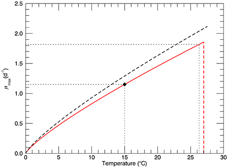
Figure 1. The black dashed line represents the dependence of maximum possible growth rate μ_max on temperature for the power law fit (Fielding, 2013). The solid red line represents power law fit through the observed growth rate of for the genotype at 15°C (1.15 d⁻¹, solid diamond ♦). The red dashed line represents the sharp drop off near 27°C observed in culture experiments (Schlüter et al., 2014). Horizontal dotted lines show values of the growth rate for temperatures 15 and 26.3°C.

Model Setup

In the model, genotypes are formulated in equal intervals along the trait axis, the growth rate μ(T) (d⁻¹), where T is the temperature. Thus, there are potential genotypes along the trait axis from μ_max = 0 to μ_max ≈ 2 d⁻¹ [corresponding to a temperature ~27°C, where the growth rate drops precipitously to zero (Fielding, 2013; Schlüter et al., 2014, Supplementary Information)].

The model is a simple exponential growth equation for each genotype i:

$\begin{array}{cc}\frac{d{N}_i}{dt}={\mu }_i(T)N_i& \left(1\right)\end{array}$

where: N_i is the number of cells in genotype i, and μⁱ(T) is the growth rate of genotype i. At 15°C the maximum possible growth rate is μ_max = 1.29 d⁻¹ (Figure 1, Fielding, 2013) and, as shown by the solid diamond in Figure 1, the realized growth rate was 1.15 d⁻¹ (Schlüter et al., 2014).

During the laboratory experiments, 10⁵ cells were transferred every 5 days from the existing batch cultures into fresh culture medium to initiate the next batch culture. In the model, the total number of cells across all genotypes N_T (= ∑_iN_i) is “normalized” to 10⁵ every timestep (0.2 d) with the same normalization factor applied to each genotype. In the standard simulations, random mutation was allowed once each day: at 15°C the growth rate was 1.15 d⁻¹, so that a mutation occurred slightly more often than 1 per generation. Each mutation produced a single cell (in 10⁵ cells). Mutations were allowed at genotypes with growth rates less than and equal to 1.15 d⁻¹. Those mutant genotypes with growth rates less than 1.15 d⁻¹ grew less quickly than the original genotype—so were not “fixed.” Because of the normalization each timestep, those mutants consisted of less than 1 cell, so were set to zero (i.e., not fixed) when they dropped to 0.1 cells. When multiple non-zero genotypes exist, the mean realized growth rate across all non-zero genotypes is given as μ_mean = (∑_iN_iμ_i)/N_T.

According to Huertas et al. (2011), “Experimental measures of mutation rates in phytoplankton range from 10⁻⁵ to 10⁻⁷ mutations per cell per generation.” So the rate of one mutation per 1.15 generations in a culture of 10⁵ cells is at the high end of the published rates. We carried out sensitivity studies with mutations occurring both more or less frequently than 1 per day: generally the simulations at lower rates resulted in a slowing down of the increase in biomass of favorable mutations but without any material change in the final results.

The magnitude of each mutation (distance of mutant genotype along the growth rate trait axis from its parent genotype) was determined from a random number generator. Two cases were simulated. First, with a “flat” pdf where the new genotype was equally probable anywhere from the lowest to highest allowed growth rate for that temperature, and, second with a Gaussian normal pdf, where the width of the distribution across genotypes was changed for different simulations. The original genotype and genotypes resulting from mutations were tracked separately. For a flat pdf, only mutations from the original genotype were allowed, since the origin was not important. For the Gaussian pdf, mutations were allowed from the original genotype or from the mutant genotypes (with a probability proportional to their relative biomasses). In both cases, only one mutation was allowed per day; sensitivity simulations with more or fewer mutations per day did not materially affect the results.

To illustrate the description above without explanation until the Results section, Figure 2A shows an initial genotype at the start of a simulation at 15°C, and Figure 2B shows a histogram of the distribution (on a logarithmic axis) of total cell biomass in each genotype—after 3 years of simulation at 15°C. The blue bars represent the relative biomass in all non-zero genotypes; “extinct” or not “fixed” genotypes were set to 10⁻⁷ as explained above.

FIGURE 2

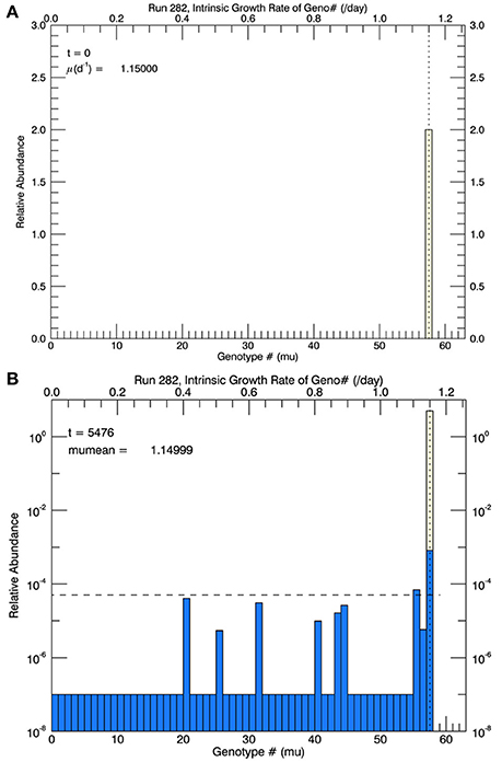
Figure 2. For the first set of simulations, at 15°C, there were 58 genotypes (#0–#57) spaced evenly in 0.02 d⁻¹ intervals along the growth rate/trait axis μ spanning the range from 0 to 1.16 d⁻¹. (A) Shows the initial genotype with μ = 1.15 d⁻¹ (the center value of the highest genotype). (B) Shows (for one particular simulation) the relative biomass (logarithmic scale) in each genotype after 3 years of mutations, where the probability of mutation was equal (“flat”) across all genotypes. After 3 years, all genotypes except #57 (and #55, which would soon become extinct) were extinct (or not “fixed”) since their simulated concentrations had become less than 1 cell (horizontal dashed line) in a culture of 10⁵ cells. When low fitness genotypes reached 1/10 of a cell, they were determined to be extinct and set to a value of 10⁻⁷.

This model considers only one trait, the maximum growth rate at a given temperature. However, two other traits were considered. First, the mortality rate μ_mort is considered to follow a power law scaling increasing as a function of temperature (Brown et al., 2004; McCoy and Gillooly, 2008; and, specifically for phytoplankton, Regaudie-de-Gioux and Duarte, 2013). However, the observations do not show any sudden drop in realized growth rate when the cultures were warmed from 15 to 26.3°C, suggesting that this scaling is inappropriate for short term changes and more appropriate for asymptotic “steady state” conditions. Second, cell size is also a function of temperature, but calculations based on the experimental results suggest that it is a minor effect. Hence, neither mortality nor cell size are considered further.

The other important environmental variable in the study of Schlüter et al. (2014) is pCO₂. While only the 400 μatm case is considered here, it is likely that higher concentrations of CO₂ result in a reduction in the height of the “fitness window,” in analogy with the “thermal window” concept for animals (Pörtner and Farrell, 2008; Denman et al., 2011).

Simulations

For the first 3 years, five replicates of the coccolithophore Emiliania huxleyi were grown in culture at 15°C for each of three pCO₂ levels: 400, 1100, and 2200 μatm. At the end of 3 years, the temperature of the cultures was raised in intervals of 1°C d⁻¹ to a final temperature of 26.3°C at which they were grown for an additional 1 year. Model simulations of the laboratory experiments with pCO₂ concentration of 400 μatm were performed as follows:

(1) Simulations at 15°C. These simulations started with a single genotype of 10⁵ cells centered on a growth rate of 1.15 d⁻¹, representing the mean observed growth rate of the five replicate cultures. Random mutation of a single cell occurred each day with a flat pdf over the growth rate trait between 0 and the maximum (for 15°C) shown by the solid red curve in Figure 1 (from Fielding, 2013). Initially there were 58 genotypes, each 0.02 d⁻¹ wide, with growth rates ranging from 0 to 1.16 d⁻¹, the maximum growth rate under the solid red curve in Figure 1. We assume that this clone/genotype was growing (during the first 3 years in culture) at its optimal rate, dependent on its original in situ temperature and location, and was not capable, under any conditions, of growing at the maximum rate observed for E. huxleyi from all locations (in Fielding, 2013).

(2) Simulations at 26.3°C, flat pdf for mutations. These simulations also started with a single genotype of 10⁵ cells centered on a growth rate of 1.15 d⁻¹, representing the mean observed growth rate of the cultures grown at 15°C for 3 years (over 1500 generations). Now there were 92 possible genotypes, with maximum growth rates ranging from 0 to 1.84 d⁻¹ (the maximum growth rate under the solid curve in Figure 1 at 26.3°C).

(3) Simulations at 26.3°C, Gaussian normal pdf for mutations. The setup was the same as in study 2, but now the magnitude of each random mutation, relative to the center of the parent genotype, followed a Gaussian normal pdf with a width s, in units of 0.02 d⁻¹ (i.e., the width of one genotype interval), which was specified at the start of the simulation.

(4) Simulations at 26.3°C, addition of a plastic response. In all simulations in study 3, for the different values of s, there was a lag of at least 60 days or generations before μ_mean, the mean growth rate of the five “replicate” simulations began to increase, contrary to the laboratory results where μ_mean increased linearly throughout year 4 without any noticeable lag or offset when the temperature was raised from 15 to 26.3°C (Schlüter et al., 2014). To remove this lag, a simple, but plausible, formulation of a plastic response (to be described later) was implemented.

Results

Simulations at 15°C

Based on arguments (Orr, 1998, 2005) critical of the concept that adaptive evolution proceeds according “micromutationism” or infinitesimal mutations as first postulated by Fisher (1930), the first set of simulations (for 3 years at 15°C) allowed for the random mutations to obey a flat pdf over the growth rate from 0 to 1.16 d⁻¹, the approximate observed growth rate μ_mean at 15°C (Figure 1). There were 58 equally wide genotypes over this space (numbered from 0 to 57). Initially they were all zero except for genotype #57, representing the measured mean growth rate 1.15 d⁻¹, shown as the solid diamond in Figure 1. The initial biomass of genotype #57 in each simulation is shown as the height of the pale yellow bar in Figure 2A.

In the simulations at 15°C, genotype #57 outcompeted all other mutant genotypes, all of which had lower growth rates (and hence lower fitness) than genotype #57. [We take the fitness of a mutant genotype m relative to the parent genotype p to be the ratio of their realized growth rates: W_mp = μ_m/μ_p, and of the relative fitness of mutant genotype i relative to mutant genotype j to be W_ij = μ_i/μ_j (Lenski et al., 1991; Schlüter et al., 2014). If W_mp (W_ij) is greater than 1, then genotype m (i) has a higher fitness than genotype p (j).] Therefore, after 3 years, in all five replicate simulations the most abundant genotype was #57 (Figure 2B), with its realized growth rate of 1.15 d⁻¹. The horizontal dashed line represents 10⁻⁵ of the total biomass, i.e., 1 cell. So by the end of the simulation, almost all genotypes except that with the highest realized growth rate (i.e., genotype #57) had biomass less than 1 cell and were effectively extinct. In the particular simulation shown in Figure 2B (one of 5 replicates) genotype #55 also had barely more than 1 cell, but it was a very recent mutation and its biomass would have quickly dropped below 1 cell, as can be seen in Figure 3. Figure 3A shows the magnitude of all the mutations over the 3 years: they are randomly distributed evenly over all genotypes between #0 and #57.

FIGURE 3

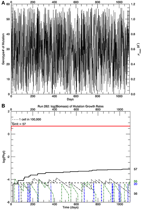
Figure 3. For the same simulation as in Figure 2B. (A) Shows the magnitude of the mutations over the 3 years of the simulation. (B) Shows the time history of the logarithm of the biomass for the original clone plus mutations to that same growth rate (red line), the proportion of that biomass which was from mutations (black line) and the other three mutant genotypes with the most biomass after 3 years: #20, #55, and #56.

Figure 3B shows the time paths of the logarithm of the biomass of genotypes 20, 55, 56, and 57. Whenever there is a mutation to genotype # 20 (blue dashed line), it quickly dies out because its fitness relative to the parent genotype #57 is small, W_{20 57} ~ 0.36. Genotype #55 (green) dies out more slowly, W_{55 57} ~ 0.97, and genotype #56 dies out even more slowly, W_{56 57} ~ 0.98. The solid red line shows the total biomass of genotype #57, consisting mostly of the original genotype (pale yellow portion in Figure 2B) plus mutations to that genotype (lower blue portion), which is also shown by the solid black line in Figure 3B. Note that the vertical scale in Figures 2B, 3B is the logarithm of biomass, so actually only 0.016% of the biomass in genotype #57 consisted of mutant cells after 3 years (all 5 replicate simulations had a similar fraction of biomass in genotype #57 ~0.02%. These cells have growth rates equal to the original clone, but they may have other genes that differ from the original clone, as pointed out by Schlüter et al. (2014). However, the simulations in the next section started with 10⁵ cells of what is assumed to be the original genotype #57, which were then warmed instantaneously (in the model) to a temperature of 26.3°C.

Simulations at 26.3°C with a Flat Pdf for Mutations

In the simulations described here, there are 92 genotypes (numbered 0 to 91) between a growth rate of 0 d⁻¹ and the maximum growth rate μ_max at 26.3°C (solid red line in Figure 1), with each genotype interval being 0.02 d⁻¹ wide as before. Thus, the highest genotype #91 is centered at 1.83 d⁻¹ with its upper limit being μ_max(26.3°C) = 1.84 d⁻¹. Similarly, μ_max(15°C) = 1.15 d⁻¹ occurs at the center of genotype #57.

Five replicate simulations at 26.3°C with a flat pdf of the magnitudes of random mutations all quickly ended up with mutant genotypes with the highest growth rate or relative fitness eventually dominating the culture. Figure 4 tracks the time history of the biomass of the four highest genotypes: 88, 89, 90, and 91 for one of the 5 simulations. A mutation to #89 occurred first (on day 31), followed by one to #88 (on day 59), then one to #91 (on day 72), and lastly one to #90 (on day 219), with the four jumps afterwards indicating subsequent mutations to this genotype. These are not the only mutations to these genotypes then, just the first ones during this simulation. Note that #88 grew more slowly than #89 (because the fitness of #89 was relatively higher, but #91 outpaced them both, for the same reason. They all outcompeted the original clone #57 because of their significantly higher relative fitness. This coexistence of four mutant clones is an example of clonal interference observed in asexual populations (e.g., Muller, 1932; Gerrish and Lenski, 1998; Imhof and Schlötterer, 2001).

FIGURE 4

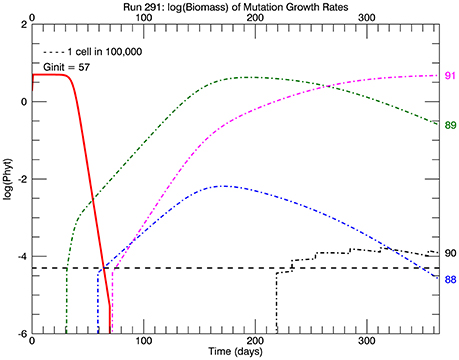
Figure 4. Time history of relative biomasses (logarithmic scale) for different genotypes for one replicate simulation after abrupt warming from 15 to 26.3°C. There are now 92 genotypes (#0–#91) spanning the trait range from 0 to 1.84 d⁻¹, the latter being the maximum growth rate at 26.3°C (solid red line, Figure 1). As before a mutation was equally probable to all genotypes (“flat” pdf). The initial genotype (representative of the culture at 15°C) was now #57 with a growth rate of 1.15 d⁻¹. The first large magnitude mutation, to genotype #89 on day 31, rapidly replaced the original genotype #57 because of its much greater relative fitness 1.56. However, the mutant genotype #91(magenta line) eventually replaced earlier genotypes #89 (green line) and #88 (blue line) because it had the highest relative fitness of all mutants.

Given enough generations, the clone with the highest fitness will dominate the culture. Reducing the mutations from once a day (slightly greater than one generation) to every other day did not affect the end result, only marginally the rate of getting there. Figure 5 shows time series of the growth rate for the five replicate simulations, each with a new “seed” for the random mutations. The timing and nature of the increase in growth rate also depends on how soon mutations at the higher genotypes occur. Regardless, in each of these simulations, there is no significant increase in growth rate in the first ~20 days, then it rapidly increases eventually to the growth rate of the highest mutant genotype. This behavior does not follow the linear increase in μ_mean from 1.15 d⁻¹ at the start of the year to 1.33 d⁻¹ (with no discernable initial lag) that was observed in the laboratory (Schlüter et al., 2014). Moreover, the asymptotic mean growth rate after 1 year in these simulations is much higher than the eventual observed mean growth rate in the laboratory experiments (shown by the blue dashed line).

FIGURE 5

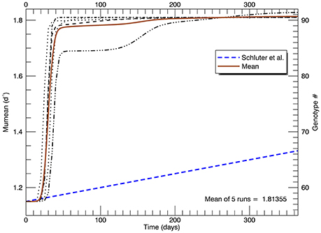
Figure 5. Time series of five replicate simulations at 26.3°C, including that in Figure 4, each with a different random seed (with a flat pdf for random mutations). The vertical axis on the left shows the growth rate (for each genotype shown on the right). The heavy brown curve shows the time history of the mean of the five replicate simulations. The heavy blue dashed line is the fitted line to the measured mean growth rate (of five replicate cultures) in the experiments (Schlüter et al., 2014).

Simulations at 26.3°C with a Gaussian Normal Pdf of Random Mutations

In the simulations with a flat pdf for random mutations, the invariable domination by mutations near the maximum possible growth rate μ_max suggests that in the laboratory experiments mutations with infinitesimal magnitudes might have been more likely (as suggested by Fisher, 1930), rather than mutations with “large” magnitudes being as likely as infinitesimal mutations (as argued by Orr, 1998, 2005, and others).

In these simulations, the magnitudes of mutations follow a Gaussian normal random pdf about the parent genotype. The width of the Gaussian normal pdf of mutation magnitude about the genotype undergoing a mutation is given by s (measured in genotype intervals of 0.02 d⁻¹). Hence, for s = 1 the distance from the center of the parent genotype interval to the outsides of the two adjacent genotypes is ±1.5s, i.e., the probability of a mutation occurring in the parent genotype or the adjoining genotypes is 86.6%. For s = 2 the distance from the center of the parent genotype interval to the outsides of the two adjacent genotypes is ±0.75s, i.e., the probability of a mutation occurring in the parent genotype or the adjoining genotypes is reduced to 54.7%.

Three sets of five replicate simulations were performed, with s = 1, 2, and 3. For s = 1, the growth rates after 1 year were well below those observed and these results are not discussed further. In Figure 6A, for s = 2, we show the distribution of biomass among genotypes after 1 year on a logarithmic scale for the replicate with the median mean growth rate. Although there appear to be about 20 genotypes in play, a linear plot of these genotypes (Figure 6B) shows that only about 4 or 5 genotypes account for almost all (at least 99%) of the biomass. We have therefore allowed only the 10 highest biomass mutant genotypes to undergo mutations themselves, with a probability inversely proportional to their relative biomass. Thus, from Figure 6B, on the next day, a mutation would be most likely be from #63, next most likely from #61, next most likely from #64 and so on, with the magnitude of each mutation determined randomly from a Gaussian normal pdf with s = 2. Figure 7A shows, for the same replicate simulation as in Figure 6, the time evolution of the biomasses of the original clone (#57, red) as well as the five mutant genotypes with the most biomass after 1 year: 61, 63, 64, 65, and 66, again demonstrating clonal interference, especially with #63 outcompeting #61, and with the higher fitness genotypes 64, 65, and 66 increasing each at a greater rate. Figure 7B shows the realized growth rate for the same simulation (heavy solid line), the mutations each day (jagged light solid line), and ± the standard deviation of the distribution of the biomasses of the active genotypes (see Figure 6A), along the trait or genotype axes (light dashed lines)

FIGURE 6

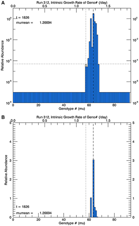
Figure 6. Results at the end of 1 year for one of five replicate simulations at 26.3°C with a Gaussian normal pdf for random mutations, with a width s = 2 genotype intervals of 0.02 d⁻¹. (A) Shows the relative biomass (on a logarithmic axis) of mutations in all genotypes after 1 year. The horizontal dotted line represents 1 cell in 10⁵ cells, and the vertical dashed line is the mean realized growth rate of the distribution. (B) Shows the same information, but for a linear biomass axis.

FIGURE 7

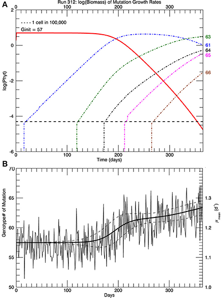
Figure 7. (A) Shows, for the same replicate simulation as in Figure 6, the time history of relative biomasses for the original genotype #57 and for the five most abundant mutant genotypes (61, 63, 64, 65, and 66) 1 year after abrupt warming from 15 to 26.3°C (similar to Figure 4). (B) Shows the time history of the mutations (light solid jagged line) about the growth rate (heavy solid line). Light dashed lines show ± one standard deviation of the distribution of biomass (Figure 6) about the growth rate/trait axis. When there are more genotypes with significant biomass, the standard deviation will be larger.

In this set of five replicate simulations with s = 2, the mean growth rate increased from 1.15 to 1.27 d⁻¹ after 1 year. In addition, the growth rate did not begin to increase until after ~110 days, roughly 125 generations (Figure 8). In the laboratory study (Schlüter et al., 2014), the realized growth rate increased, more or less linearly without discernible lag, to a value (from their fitted line) of 1.33 d⁻¹ at the end of 1 year. Thus, the increase in realized growth rate in these simulations was too small and the initial lag of ~110 days was unrealistic.

FIGURE 8

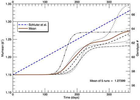
Figure 8. Time series of all five replicate simulations at 26.3°C with a Gaussian normal pfd (with s = 2) for mutations about the mean growth rate Note that the realized growth rate did not increase significantly in any simulation until after ~110 days. The blue dashed line is as in Figure 5 (note change of scale on the vertical axis).

Another set of five simulations was performed with s = 3. Figure 9 shows the time path of the mean growth rate for each of the five replicate simulations (light lines), the overall mean growth rate (brown solid line) and the fitted linear increase in growth rate from the experiments (blue dashed line, Schlüter et al., 2014). After 1 year, the mean growth rate was 1.47 d⁻¹ (range 1.39–1.69 d⁻¹), exceeding that in the laboratory experiment. These simulations tend to exhibit lags of ~70–130 days followed by plateaus, especially the simulation with the highest growth rate after 1 year. In that simulation, after ~70 days the growth rate increased steeply to a plateau ~1.33 d⁻¹ (genotype #66), then at ~200 days it increased again to a plateau ~1.55 d⁻¹ (genotype #77) followed by another steep rise starting at ~320 days. Figure 10A shows the distribution of genotypes after 1 year for this simulation: here there were 12 genotypes with biomasses greater than 1 cell. Figure 10B tracks the time history of the simulation for genotypes 66, 77, 81, 82, and 85. The first large magnitude mutation from the parent genotype #57 to genotype #66 (on day 15) is rare (3s) but possible for a Gaussian normal pdf with s = 3; the second from #66 to #77 (on day 149) is also rare but possible. Figure 10B again shows clonal interference, as mutants with higher relative fitness eventually out-compete less fit mutants (cf. Figures 8, 9 in Gerrish and Lenski, 1998).

FIGURE 9

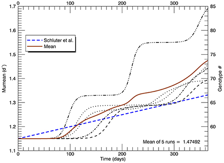
Figure 9. Time series of the realized growth rates for all five replicate simulations with s = 3 (light broken lines), the mean growth rate for the five simulations (solid brown line), and the fitted (dashed blue) line to the experimental results as in Figures 5, 8 (again note the change of scale on the vertical axis).

FIGURE 10

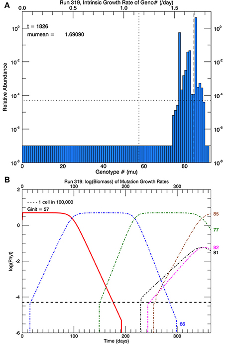
Figure 10. Results for one of five replicate simulations with s = 3, the one with the highest growth rate (1.69 d⁻¹) at the end of 1 year. All other parameters are the same as in Figures 6–8. (A) Shows the relative biomass of mutations in all genotypes after 1 year. (B) Shows the time history of the original genotype #57 (solid red line) and five other genotypes (66, 77, 81, 82, and 85). Mutations with large magnitude to #66 and later to #77 each became dominant, resulting in plateaus lasting ~60 days (see Figure 9).

To summarize the results of this set of simulations, the overall mean growth rate increased roughly linearly after about 70 days, but again among the replicate simulations there was a lag of ~70–130 days before the growth rate(s) start to increase, contrary to the experimental data (Schlüter et al., 2014).

Discussion

Three-Year Simulations at 15°C

Initially, the model was set up with 58 genotypes (each 0.02 d⁻¹ wide) spanning the range of possible growth rates at 15°C from 0 to ~1.16 d⁻¹ (Figure 2 and Fielding, 2013). Mutations were equally probable (a “flat” pdf) to all 58 genotypes (#0 to #57) under the assumption that the original genotype #57 was the genotype with the highest possible growth rate and hence the maximum relative fitness. So only mutations to that same genotype survived or were “fixed,” while mutations to other genotypes (#0 to #56), all with lower relative fitness, became extinct (or failed to be “fixed”), as shown in Figures 2, 3. At the end of the 3 years, in all five replicate simulations, mutations to genotype #57 contributed ~0.02% to the total biomass shown in that genotype. Although these cells had the same growth rate as the original clones, they presumably possessed other genes that apparently did not affect their growth rate at 15°C.

Time Lag in Growth Rate Response to Mutations

Simulations at 26.3°C had 92 possible genotypes, each of width 0.02 d⁻¹, spanning the growth rates between 0 and 1.84 d⁻¹, the maximum possible growth rate for this clone (the value of the red line in Figure 1 at 26.3°C). The initial genotype was still #57, assumed to be the single genotype existing after 3 years of growing at 15°C, ignoring the ~0.02% of the cells that were mutants in the simulations but with the same growth rate at 15°C. All simulations exhibited a time lag after the temperature shift from 15°C before there was any significant increase in the realized growth rate, which was not observed in the laboratory experiments of Schlüter et al. (2014).

For a flat pdf of random mutations, the genotype created from the largest magnitude favorable mutation eventually dominated and replaced the original genotype. Usually, after 1 year the dominant genotype is #90 or #91 (Figures 4, 5). Figure 5 shows that there is typically a lag of ~15–30 days (~17–34 generations) before the realized growth rate starts to increase significantly. Then very quickly (over ~20 days) the growth rate climbs rapidly to that for the highest mutant genotype, where it remains for the rest of the year unless there is a subsequent mutation to a higher genotype. This behavior, two plateaus separated by an abrupt increase from the first to the second, is completely inconsistent with, and with a much larger final growth rate than, the final fitted growth rate from the laboratory experiments.

For the flat pdf, each mutation has a 62% chance of having a relative fitness less than that of the original clone (57 of 92 possible genotypes). If the rate of mutations were to decrease by a factor of 10, then the lag time would be 10 times longer, but the time for a given favorable mutation to increase would be the same because it is a function of the generation time or growth rate.

It was concluded from these simulations that an initial lag followed by an abrupt increase in growth rate results from allowing mutations of the largest magnitude to have the same probability as mutations of the smallest magnitude. If small magnitude mutations were to have a much higher probability than large magnitude mutations, then possibly the transition to higher grow rates after increasing the temperature to 26.3°C would be more gradual and continuous. To allow for mutations of very small magnitude, in subsequent simulations the magnitude of each mutation along the trait axis was chosen randomly from a Gaussian normal pdf, N(μ_max, s) in statistical notation, centered on the growth rate of the parent genotype, with a width along the trait axis scaled by the standard deviation s (in genotype intervals).

The first set of five simulations shown here, with s = 2 genotypes wide, generated a much too small increase in mean growth rate μ_mean, reaching only 1.27 d⁻¹ compared with the fitted value of 1.33 d⁻¹ from the laboratory experiments. Again, the simulations show a long lag of ~110 days before any significant increase occurred (Figure 8). A second set of five simulations with s = 3 was then performed (Figure 9). A larger number of genotypes were generated from mutations, with many of them still viable (1 cell or more) at the end of 1 year (Figure 10). The mean growth rate of the five replicate simulations increased more or less linearly for the latter two thirds of the year, with a slope roughly double that observed. But there still remained a lag of ~70 days before the mean growth rate started to increase. Overall, for a larger s, i.e., larger magnitude mutations, the lag time was shorter. For s = 1, 2, and 3, the lag time was respectively ~150, ~120, and ~70 days. Clearly, adaptive evolution by genetic mutations, modeled in the manner described here, cannot alone explain the laboratory results (Schlüter et al., 2014) because all simulations were characterized by initial lags upon warming to 26.3°C.

A “Plastic” Response to Abrupt Temperature Change?

A possible explanation for the immediate continuous increase in observed growth rate after increasing the temperature from 15 to 26.3°C is that it was a “plastic” response of the cells to their changing environment. The idea of plasticity “buying time” for genetic adaptation to take place is central to the concept of “plastic rescue” avoiding extinction (e.g., Lande, 2009; Chevin et al., 2010; Kopp and Matuszewski, 2014). There are many definitions of plasticity: Whitman and Agrawal (2009) list 11, but perhaps their simplest is “Phenotypic plasticity” is “the capacity of a single genotype to exhibit variable phenotypes in different environments ….” According to Reusch (2014), reviewing evidence of plasticity in marine animals and plants: “Phenotypic plasticity broadly defines the adjustment of phenotypic values of genotypes depending on the environment, without genetic changes.”

Most studies of plasticity compare different phenotypes of the same genotype in different environments. More relevant in our case would be studies that consider the temporal change in phenotypic properties of a given genotype in response to a change (continuous or abrupt) in its environment, but such studies are rare. And different species generally have different plastic responses to the same change in environment (different “reaction norms,” (e.g., Pigliucci, 2005; Whitman and Agrawal, 2009; Reusch, 2014). There is no clear information on how plasticity might be modeled in this case, especially what ultimately limits the rate and magnitude of plastic response. Currently, both the energetic costs and limits of plasticity are research questions of considerable interest (e.g., DeWitt et al., 1998; Pigliucci, 2005).

Given that the generation time of E. huxleyi in the laboratory experiments was less than 1 day, a plastic response would have to be “transgenerational” or heritable, for which there is mounting evidence in animals (Munday, 2014; Walsh et al., 2014), in clonal plants (e.g., Latzel and Klimešová, 2010), and in phytoplankton (Schaum et al., 2013; Schaum and Collins, 2014). For asexual reproduction the hypothesized mechanism is “epigenetic inheritance” whereby an environmental change causes genes to be expressed, which continue to be expressed in succeeding generations if the environmental change continues (Latzel and Klimešová, 2010; Schaum et al., 2013; Schaum and Collins, 2014; van Oppen et al., 2015). In the laboratory experiments of Schlüter et al. (2014), it is assumed that the change in temperature from 15 to 26.3°C caused the expression of an existing gene in essentially all cells in the culture in the first and succeeding generations which mediated a slow increase in growth rate, without the lag that would result from the favorable mutation of a single cell dividing sufficiently often to start to compete with the original population.

Here we assume that the plasticity is heritable, and model it as a first order restoring function without lag:

$\begin{array}{cc}\frac{d{\mu }_i(t)}{dt}=({\mu }_{\text{max}}(i)-{\mu }_i(t))/T& \left(2\right)\end{array}$

where μ_i(t) is the realized growth rate and μ_max(i) is the maximum growth rate, both for the initial genotype i, according to the power law fit (Fielding, 2013) through the original growth rate at 15°C (solid red line in Figure 1). T (or τ) is the “e-folding” time for the response. The assumed mechanism is that because of energy costs the plastic response of a given genotype i cannot exceed its μ_max(i) value for 15°C, even though it is now at a higher temperature. The rate at which μ_i(t) approaches μ_max(i) decreases as it gets closer, the logic being that the larger the plastic response, the more energy that is required.

The solution to the ordinary differential Equation (2) is standard:

$\begin{array}{cc}{\mu }_i(t)=({\mu }_i(0)-{\mu }_{\text{max}}(i)){\text{e}}^{-t/T}+{\mu }_{\text{max}}(i)& \left(3\right)\end{array}$

This function has the form shown Figure 11, where the dashed curve shows the full function to its asymptote. The solid curve has a T value set to 281 d, so that the initial slope of Equation (3) at small t is equal to the slope of the linear fit to the observations over 1 year (Figure 1A in Schlüter et al., 2014). For the initial genotype, μ_max = 1.29 d⁻¹, so that the observed (fitted) growth rate after 1 year of 1.33 d⁻¹ could not be reached by means of plasticity alone. In fact for the value chosen for T, the plastic response at the end of 1 year would result in a mean growth rate of only 1.25 d⁻¹ (solid curve, Figure 11).

FIGURE 11

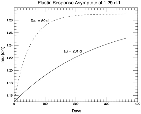
Figure 11. The proposed plastic response over time of genotype #57 to the temperature change from 15 to 26.3°C. The asymptote is μ_max for 15°C (shown in the dashed curve). The initial slope in the solid curve (used in the simulations) is set to match the slope of the line fitted to the 1 year of measured growth rates from the laboratory experiments in Schlüter et al. (2014).

Three sets of five replicate simulations were then performed at 26.3°C with s = 2, 2.5, and 3, but with a plastic response of the original genotype. Now the growth rate of the initial genotype (initially μ_i(0) = 1.15 d⁻¹) increased with time according to Equation (3). As its growth rate increased, the biomass of the original genotype was added to any in the appropriate growth rate interval that had accumulated from mutations. Due to the plastic response, the original genotype had moved from #57 to #62 on the growth rate axis after 1 year. Figure 12A shows the results of 1 replicate simulation with s = 2.5; in all five replicate simulations with s = 2.5, the original genotype represented most of the biomass in that interval. Figure 12B shows the time evolution of the five other genotypes with the most biomass after 1 year: clonal interference between genotypes 63, 64, and 66. Genotype #66, because it had the highest relative fitness, outcompeted genotypes 63, and 64, even though they had mutated earlier. Figure 13A shows the time history of the growth rates for all five replicate simulations, the ensemble mean growth rate (solid brown line), and the (dashed blue) line fitted to the laboratory results. The plastic response eliminated the initial lag in the increase of the growth rate, consistent with the observations. The ensemble growth rate after 1 year was 1.34 d⁻¹ (slightly greater than that of the observations, 1.33 d⁻¹). In Figure 13B, simulated random measurement error has been added to the simulated overall mean growth rate, for comparison with the observations (Figure 1A in Schlüter et al., 2014). Thus, the plastic response, as formulated, removed the lag in response present in all previous simulations, giving time for mutations to new genotypes eventually to dominate the culture toward the end of the year. In addition to the maximum growth rate, the only other trait reported on by Schlüter et al. (2014) was cell diameter. The cell diameter was significantly smaller (~10%) at 26.3°C, but only for the cultures grown at the “ambient” level of pCO₂: 400 μatm.

FIGURE 12

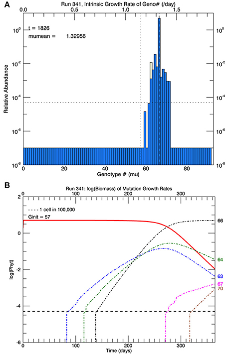
Figure 12. Results for one simulation (with s = 2.5) that includes the plastic response (Figure 11). In (A), the vertical dotted line shows the growth rate of the original genotype and the position on the x-axis of the light yellow bar shows where the growth rate of the initial genotype (#57) has reached (genotype #62) with the growth rates shown on the upper x-axis. (B) Shows the time series of the relative biomass of the different genotypes: the original genotype (#57, solid red line), and the five most abundant genotypes at the end of 1 year (63, 64, 66, 67, and 70). Genotype #66 has become the dominant genotype (highest peak in A) due to its higher fitness relative to #57, although eventually the mutant genotype #70 would replace #66.

FIGURE 13

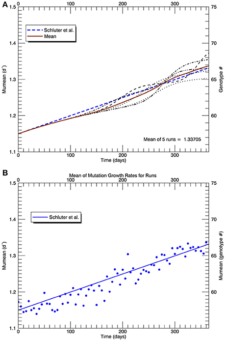
Figure 13. Similar to Figure 10, (A) shows the time series of all five replicate simulations (s = 2.5) with the plastic response implemented as in Figure 11 (light curves), the mean realized growth rate for the five replicate simulations (solid brown curve), and (as in Figures 5, 8, 10) the (dashed blue) line fitted to the experimental results (Schlüter et al., 2014). (B) shows (blue) points along the mean (brown) curve with simulated random “measurement errors,” and the fit to the experimental results (solid blue line), for comparison with Figure 1A in Schlüter et al. (2014).

Effects of Multiple Stressors

Schlüter et al. (2014) maintained cultures of Emiliania huxleyi, all originating from the same single cell, at three different pCO₂ levels for 4 years, increasing the temperature from 15 to 26.3°C at the end of the third year. Although the growth rate at 15°C decreased with increasing pCO₂, the growth rate increase over the last year (at 26.3°C) was greater at successive higher pCO₂ levels, such that the growth rates at the end of the experiment were closer together than during the first 3 years, suggesting that at the higher temperature, the cells were affected less by CO₂ concentration. Without some information about energy costs of adaptation, it is not clear how to model either the effects of mutation (or of plasticity) in response to two simultaneous stressors.

Conclusions

Modeling even the adaptive response to abrupt change in a single environmental variable in an asexual phytoplankton population of a single trait led to unexpected results. If this model is a valid representation of the experimental results of Schlüter et al. (2014), then several conclusions pertain:

(1) The largely linear increase over 1 year in measured growth rate without an initial lag after an abrupt increase in temperature cannot be explained on the basis of genetic mutation alone. The caveat (mentioned by Schlüter et al., 2014) is that there were cells in the culture at 15°C after 3 years, which were mutants with the same growth rate 1.15 d⁻¹ but with some different genes that would possibly allow them to respond differently to the increase in temperature to 26.3°C. In the model simulations at 15°C, after 3 years these cells comprised only ~0.02% of the culture, suggesting that some lag would still occur after the switch to a warmer temperature.

(2) Mutation may occur frequently, i.e., close to every generation, but not all mutations are favorable, i.e., have a higher relative greater fitness than the original culture, and all mutations with a relative fitness less than the original culture are not “fixed” and hence become extinct.

(3) Future models of plasticity and effects of multiple stressors require some knowledge and formulation of “costs vs. benefits” in order to determine rates and ultimate limits in plastic response (e.g., Sokolova, 2013).

Author Contributions

All research and manuscript writing and preparation were carried out by the author.

Funding

The author received no research funds for this work. The Canadian Centre for Climate Modelling and Analysis of Environment and Climate Change Canada and the University of Victoria provided office space and network support.

Conflict of Interest Statement

The author declares that the research was conducted in the absence of any commercial or financial relationships that could be construed as a potential conflict of interest.

Acknowledgments

The author benefitted from discussions with other participants at the 2014 and 2016 Gordon Research Conferences on Ocean Global Change Biology, and from discussions with J. R. Christian. Y. Zhang, U. Riebesell, and T. Reusch provided their growth rate vs. temperature data and fitted thermal response functions from Zhang et al. (2014). The author wishes to thank the two reviewers for their constructive and helpful comments, which improved the manuscript immeasurably.

References

Bissinger, J. E., Montagnes, D. J. S., Sharples, J., and Atkinson, D. (2008). Predicting marine phytoplankton maximum growth rates from temperature: improving on the Eppley curve using quantile regression. Limnol. Oceanogr. 53, 487–493. doi: 10.4319/lo.2008.53.2.0487

CrossRef Full Text | Google Scholar

Brown, J. H., Gillooly, J. F., Allen, A. P., Savage, V. M., and West, G. B. (2004). Toward a metabolic theory of ecology. Ecology 85, 1771–1789. doi: 10.1890/03-9000

CrossRef Full Text | Google Scholar

Chevin, L.-M., Lande, R., and Mace, G. M. (2010). Adaptation, plasticity, and extinction in a changing environment: towards a predictive theory. PLoS Biol. 8:e1000357. doi: 10.1371/journal.pbio.1000357

PubMed Abstract | CrossRef Full Text | Google Scholar

Chust, G., Allen, J. I., Bopp, L., Schrum, C., Holt, J., Tsiaras, K., et al. (2014). Biomass changes and trophic amplification of plankton in a warmer ocean. Glob. Chang. Biol. 20, 2124–2139. doi: 10.1111/gcb.12562

PubMed Abstract | CrossRef Full Text | Google Scholar

Collins, M., Knutti, R., Arblaster, J., Dufresne, J.-L., Fichefet, T., Friedlingstein, P., et al. (2013). “Long-term climate change: projections, commitments and irreversibility,” in Climate Change 2013: The Physical Science Basis. Contribution of Working Group I to the Fifth Assessment Report of the Intergovernmental Panel on Climate Change, eds T. F. Stocker, D. Qin, G.-K. Plattner, M. Tignor, S. K. Allen, J. Boschung, et al. (Cambridge; New York, NY: Cambridge University Press), 1029–1136.

Collins, S. (2011). Many possible worlds: expanding the ecological scenarios in experimental evolution. Evol. Biol. 38, 3–14. doi: 10.1007/s11692-010-9106-3

CrossRef Full Text | Google Scholar

Collins, S., and Bell, G. (2004). Phenotypic consequences of 1,000 generations of selection at elevated CO₂ in a green alga. Nature 431, 566–569. doi: 10.1038/nature02945

PubMed Abstract | CrossRef Full Text | Google Scholar

Collins, S., Sültemeyer, D., and Bell, G. (2006). Rewinding the tape: selection of algae adapted to high CO₂ at current and pleistocene levels of CO₂. Evolution 60, 1392–1401. doi: 10.1111/j.0014-3820.2006.tb01218.x

PubMed Abstract | CrossRef Full Text | Google Scholar

Collins, S., Rost, B., and Rynearson, T. A. (2014). Evolutionary potential of marine phytoplankton under ocean acidification. Evol. Appl. 7, 140–155. doi: 10.1111/eva.12120

PubMed Abstract | CrossRef Full Text | Google Scholar

Daniels, C. J., Sheward, R. M., and Poulton, A. J. (2014). Biogeochemical implications of comparative growth rates of Emiliania huxleyi and Coccolithus species. Biogeosciences 11, 6915–6925. doi: 10.5194/bg-11-6915-2014

CrossRef Full Text | Google Scholar

Denman, K., Christian, J. R., Steiner, N., Poertner, H.-O., and Nojiri, Y. (2011). Potential impacts of future ocean acidification on marine ecosystems and fisheries: current knowledge and recommendations for future research. ICES J. Mar. Sci. 68, 1019–1029. doi: 10.1093/icesjms/fsr074

CrossRef Full Text | Google Scholar

DeWitt, T. J., Sih, A., and Wilson, D. S. (1998). Costs and limits of phenotypic plasticity. Trends Ecol. Evol. (Amst). 13, 77–81. doi: 10.1016/S0169-5347(97)01274-3

PubMed Abstract | CrossRef Full Text | Google Scholar

Eppley, R. W. (1972). Temperature and phytoplankton growth in the sea. Fish. Bull. 70, 1063–1085.

Google Scholar

Gerrish, P. J., and Lenski, R. E. (1998). The fate of competing beneficial mutations in an asexual population. Genetica 102–103, 127–144. doi: 10.1023/A:1017067816551

PubMed Abstract | CrossRef Full Text | Google Scholar

Fielding, S. R. (2013). Emiliania huxleyi specific growth rate dependence on temperature. Limnol. Oceanogr. 58, 663–666. doi: 10.4319/lo.2013.58.2.0663

CrossRef Full Text | Google Scholar

Fisher, R. A. (1930). The Genetical Theory of Natural Selection. Oxford: Oxford University Press.

Google Scholar

Hagino, K., Bendif, E. M., Young, J. R., Kogame, K., Probert, I., Takano, Y., et al. (2011). New evidence for morphological and genetic variation in the cosmopolitan coccolithophore Emiliania huxleyi (prymnesiophyceae) from the cox1b-atp4 genes1. J. Phycol. 47, 1164–1176. doi: 10.1111/j.1529-8817.2011.01053.x

CrossRef Full Text | Google Scholar

Hoegh-Guldberg, O., Cai, R., Poloczanska, E. S., Brewer, P. G., Sundby, S., Hilmi, K., et al. (2014). “The ocean,” in Climate Change 2014: Impacts, Adaptation, and Vulnerability. Part B: Regional Aspects. Contribution of Working Group II to the Fifth Assessment Report of the Intergovernmental Panel of Climate Change, eds V. R. Barros, C. B. Field, D. J. Dokken, M. D. Mastrandrea, K. J. Mach, T. E. Bilir, et al. (Cambridge; New York, NY: Cambridge University Press), 1655–1731.

Huertas, I. E., Rouco, M., López-Rodas, V., and Costas, E. (2011). Warming will affect phytoplankton differently: evidence through a mechanistic approach. Proc. Biol. Sci. 278, 3534–3543. doi: 10.1098/rspb.2011.0160

PubMed Abstract | CrossRef Full Text | Google Scholar

Imhof, M., and Schlötterer, C. (2001). Fitness effects of advantageous mutations in evolving Escherichia coli populations. Proc. Natl. Acad. Sci. U.S.A. 98, 1113–1117. doi: 10.1073/pnas.98.3.1113

PubMed Abstract | CrossRef Full Text | Google Scholar

Kopp, M., and Matuszewski, S. (2014). Rapid evolution of quantitative traits: theoretical perspectives. Evol. Appl. 7, 169–191. doi: 10.1111/eva.12127

PubMed Abstract | CrossRef Full Text | Google Scholar

Lande, R. (2009). Adaptation to an extraordinary environment by evolution of phenotypic plasticity and genetic assimilation. J. Evol. Biol. 22, 1435–1446. doi: 10.1111/j.1420-9101.2009.01754.x

PubMed Abstract | CrossRef Full Text | Google Scholar

Latzel, V., and Klimešová, J. (2010). Transgenerational plasticity in clonal plants. Evol. Ecol. 24, 1537–1543. doi: 10.1007/s10682-010-9385-2

CrossRef Full Text | Google Scholar

Lenski, R., Rose, M., Simpson, S., and Tadler, S. (1991). Long-term experimental evolution in Escherichia-coli. 1. Adaptation and divergence during 2,000 generations. Am. Nat. 138, 1315–1341. doi: 10.1086/285289

CrossRef Full Text | Google Scholar

Litchman, E., Edwards, K. F., Klausmeier, C. A., and Thomas, M. K. (2012). Phytoplankton niches, traits and eco-evolutionary responses to global environmental change. Mar. Ecol. Prog. Ser. 470, 235–248. doi: 10.3354/meps09912

CrossRef Full Text | Google Scholar

Litchman, E., and Klausmeier, C. A. (2008). Trait-based community ecology of phytoplankton. Annu. Rev. Ecol. Evol. Syst. 39, 615–639. doi: 10.1146/annurev.ecolsys.39.110707.173549

CrossRef Full Text | Google Scholar

Lohbeck, K. T., Riebesell, U., and Reusch, T. B. H. (2012). Adaptive evolution of a key phytoplankton species to ocean acidification. Nat. Geosci. 5, 346–351. doi: 10.1038/ngeo1441

CrossRef Full Text | Google Scholar

Mackas, D. L., Batten, S., and Trudel, M. (2007). Effects on zooplankton of a warmer ocean: recent evidence from the Northeast Pacific. Prog. Oceanogr. 75, 223–252. doi: 10.1016/j.pocean.2007.08.010

CrossRef Full Text | Google Scholar

McCoy, M. W., and Gillooly, J. F. (2008). Predicting natural mortality rates of plants and animals. Ecol. Lett. 11, 710–716. doi: 10.1111/j.1461-0248.2008.01190.x

PubMed Abstract | CrossRef Full Text | Google Scholar

Muller, H. J. (1932). Some genetic aspects of sex. Am. Nat. 66, 118–138. doi: 10.1086/280418

CrossRef Full Text | Google Scholar

Munday, P. L. (2014). Transgenerational acclimation of fishes to climate change and ocean acidification. F100Prime Rep. 6:99. doi: 10.12703/P6-99

PubMed Abstract | CrossRef Full Text | Google Scholar

Norberg, J. (2004). Biodiversity and ecosystem functioning: a complex adaptive systems approach. Limnol. Oceanogr. 49, 1269–1277. doi: 10.4319/lo.2004.49.4_part_2.1269

CrossRef Full Text | Google Scholar

Norberg, J., Swaney, D. P., Dushoff, J., Lin, J., Casagrandi, R., and Levin, S. A. (2001). Phenotypic diversity and ecosystem functioning in changing environments: a theoretical framework. Proc. Natl. Acad. Sci. U.S.A. 98, 11376–11381. doi: 10.1073/pnas.171315998

PubMed Abstract | CrossRef Full Text | Google Scholar

Norberg, J., Urban, M. C., Vellend, M., Klausmeier, C. A., and Loeuille, N. (2012). Eco-evolutionary responses of biodiversity to climate change. Nat. Clim. Chang. 2, 747–751. doi: 10.1038/nclimate1588

CrossRef Full Text | Google Scholar

Orr, H. A. (1998). The population genetics of adaptation: the distribution of factors fixed during adaptive evolution. Evolution 52, 935–949. doi: 10.2307/2411226

CrossRef Full Text | Google Scholar

Orr, H. A. (2005). The genetic theory of adaptation: a brief history. Nat. Rev. Genet. 6, 119–127. doi: 10.1038/nrg1523

PubMed Abstract | CrossRef Full Text | Google Scholar

Pigliucci, M. (2005). Evolution of phenotypic plasticity: where are we going now? Trends Ecol. Evol. 20, 481–486. doi: 10.1016/j.tree.2005.06.001

PubMed Abstract | CrossRef Full Text | Google Scholar

Planque, B. (2015). Projecting the future state of marine ecosystems, “la grande illusion”? IICES J. Mar. Sci. 73, 204–208. doi: 10.1093/icesjms/fsv155

CrossRef Full Text | Google Scholar

Pörtner, H. O., and Farrell, A. P. (2008). Physiology and climate change. Science 322, 690–692. doi: 10.1126/science.1163156

PubMed Abstract | CrossRef Full Text | Google Scholar

Pörtner, H.-O., Karl, D., Boyd, P. W., Cheung, W., Lluch-Cota, S. E., Nojiri, Y., et al. (2014). “Ocean systems,” in Climate Change 2014: Impacts, Adaptation, and Vulnerability. Part A: Global and Sectoral Aspects. Contribution of Working Group II to the Fifth Assessment Report of the Intergovernmental Panel of Climate Change, eds C. B. Field, V. R. Barros, D. J. Dokken, K. J. Mach, M. D. Mastrandrea, T. E. Bilir, et al. (Cambridge; New York, NY: Cambridge University Press), 411–484.

Read, B. A., Kegel, J., Klute, M. J., Kuo, A., Lefebvre, S. C., Maumus, F., et al. (2013). Pan genome of the phytoplankton Emiliania underpins its global distribution. Nature 499, 209–213. doi: 10.1038/nature12221

PubMed Abstract | CrossRef Full Text | Google Scholar

Regaudie-de-Gioux, A., and Duarte, C. M. (2013). Global patterns in oceanic planktonic metabolism. Limnol. Oceanogr. 58, 977–986. doi: 10.4319/lo.2013.58.3.0977

CrossRef Full Text | Google Scholar

Reusch, T. B. H. (2014). Climate change in the oceans: evolutionary versus phenotypically plastic responses of marine animals and plants. Evol. Appl. 7, 104–122. doi: 10.1111/eva.12109

PubMed Abstract | CrossRef Full Text | Google Scholar

Reznick, D. N., Shaw, F. H., Rodd, F. H., and Shaw, R. G. (1997). Evaluation of the rate of evolution in natural populations of guppies (Poecilia reticulata). Science 275, 1934–1937. doi: 10.1126/science.275.5308.1934

PubMed Abstract | CrossRef Full Text | Google Scholar

Rhein, M., Rintoul, S. R., Aoki, S., Campos, E., Chambers, D., Feely, R. A., et al. (2013). “Observations: ocean,” in Climate Change 2013: The Physical Science Basis. Contribution of Working Group I to the Fifth Assessment Report of the Intergovernmental Panel on Climate Change, eds T. F. Stocker, D. Qin, G.-K. Plattner, M. Tignor, S. K. Allen, J. Boschung, et al. (Cambridge; New York, NY: Cambridge University Press), 255–316.

Schaum, C. E., and Collins, S. (2014). Plasticity predicts evolution in a marine alga. Proc. R. Soc. B 281:20141486. doi: 10.1098/rspb.2014.1486

PubMed Abstract | CrossRef Full Text | Google Scholar

Schaum, E., Rost, B., Millar, A. J., and Collins, S. (2013). Variation in plastic responses of a globally distributed picoplankton species to ocean acidification. Nat. Clim. Chang. 3, 298–302. doi: 10.1038/nclimate1774

CrossRef Full Text | Google Scholar

Schlüter, L., Lohbeck, K. T., Gutowska, M. A., Groger, J. P., Riebesell, U., and Reusch, T. B. H. (2014). Adaptation of a globally important coccolithophore to ocean warming and acidification. Nat. Clim. Change 4, 1024–1030. doi: 10.1038/nclimate2379

CrossRef Full Text | Google Scholar

Simpson, S. D., Jennings, S., Johnson, M. P., Blanchard, J. L., Schön, P.-J., Sims, D. W., et al. (2011). Continental shelf-wide response of a fish assemblage to rapid warming of the sea. Curr. Biol. 21, 1565–1570. doi: 10.1016/j.cub.2011.08.016

PubMed Abstract | CrossRef Full Text | Google Scholar

Sokolova, I. M. (2013). Energy-limited tolerance to stress as a conceptual framework to integrate the effects of multiple stressors. Integr. Comp. Biol. 53, 597–608. doi: 10.1093/icb/ict028

PubMed Abstract | CrossRef Full Text | Google Scholar

Sorte, C. J. B., Williams, S. L., and Carlton, J. T. (2010). Marine range shifts and species introductions: comparative spread rates and community impacts. Glob. Ecol. Biogeogr. 19, 303–316. doi: 10.1111/j.1466-8238.2009.00519.x

CrossRef Full Text | Google Scholar

van Oppen, M. J. H., Oliver, J. K., Putnam, H. M., and Gates, R. D. (2015). Building coral reef resilience through assisted evolution. Proc. Natl. Acad. Sci. U.S.A. 112, 2307–2313. doi: 10.1073/pnas.1422301112

PubMed Abstract | CrossRef Full Text | Google Scholar

Walsh, M. R., Whittington, D., and Funkhouser, C. (2014). Thermal transgenerational plasticity in natural populations of Daphnia. Integr. Comp. Biol. 54, 822–829. doi: 10.1093/icb/icu078

PubMed Abstract | CrossRef Full Text | Google Scholar

Watabe, N., and Wilbur, K. (1966). Effects of temperature on growth calcification and coccolith form in Coccolithus huxleyi (coccolithineae). Limnol. Oceanogr. 11, 567–575. doi: 10.4319/lo.1966.11.4.0567

CrossRef Full Text | Google Scholar

Whitman, D. W., and Agrawal, A. A. (2009). “What is phenotypic plasticity and why is it important?” in Phenotypic Plasticity of Insects : Mechanisms and Consequences, eds D. W. Whitman, and T. N. Ananthakrishnan (Enfield, NH: Science Publishers), 1–63.

Winter, A., Henderiks, J., Beaufort, L., Rickaby, R. E. M., and Brown, C. W. (2014). Poleward expansion of the coccolithophore Emiliania huxleyi. J. Plankton Res. 36, 316–325. doi: 10.1093/plankt/fbt110

CrossRef Full Text | Google Scholar

Wong, P. P., Losada, I. J., Gattuso, J.-P., Hinkel, J., Khattabi, A., McInnes, K. L., et al. (2014). “Coastal systems and low-lying areas,” in Climate Change 2014: Impacts, Adaptation, and Vulnerability. Part A: Global and Sectoral Aspects. Contribution of Working Group II to the Fifth Assessment Report of the Intergovernmental Panel of Climate Change, eds C. B. Field, V. R. Barros, D. J. Dokken, K. J. Mach, M. D. Mastrandrea, T. E. Bilir, et al. (Cambridge; New York, NY: Cambridge University Press), 361–409.

Zhang, Y., Klapper, R., Lohbeck, K. T., Bach, L. T., Schulz, K. G., Reusch, T. B. H., et al. (2014). Between- and within-population variations in thermal reaction norms of the coccolithophore Emiliania huxleyi. Limnol. Oceanogr. 59, 1570–1580. doi: 10.4319/lo.2014.59.5.1570

CrossRef Full Text | Google Scholar