Plastic Pollution Patterns in Offshore, Nearshore and Estuarine Waters: A Case Study from Perth, Western Australia
 Sara Hajbane
 Charitha B. Pattiaratchi
- 1School of Civil, Environmental and Mining Engineering, and UWA Oceans Institute, University of Western Australia, Crawley, WA, Australia
- 2School of Earth and Environment, University of Western Australia, Crawley, WA, Australia
Plastic pollution in marine surface waters is prone to high spatial and temporal variability. As a result increases in pollution over time are hard to detect. Selecting areas, based on variable oceanographic and climatological drivers, rather than distance-based approaches, is proposed as a means to better understand the dynamics of this confounding variability in coastal environments. A pilot study conducted in Perth metropolitan waters aimed to explore the applicability of this approach, whilst quantifying levels of plastic pollution in an understudied part of the world. Pollution ranged from 950 to 60,000 pieces km−2 and was dominated by fishing line. Offshore concentrations were highest with strongest Leeuwin Current flow, in the estuary immediately after rainfall, and increased in the nearshore after estuarine outfall. Results elucidated significant relationships between physical drivers and concentration changes and therefore their roles in increasing or decreasing local plastic pollution. Such observations can form the basis for predicting peak pollution periods and inform targeted mitigation.
Introduction
Plastic pollution in the surface of the ocean has become an issue of growing concern since it was first observed and documented in the open ocean in the early 1970s (Carpenter and Smith, 1972; Andrady, 2011). Large-scale and long-term studies with the aim of quantifying concentrations and distributions are growing rapidly to further our knowledge on the state of plastic pollution (Hidalgo-Ruz et al., 2012; do Sul and Costa, 2014). Various gyre-wide and multi-year comparisons have been conducted in the last decade to understand the spread and increase in pollution at sea (Thompson et al., 2004; Law et al., 2010; Eriksen et al., 2013). Whilst subtropical gyres as major accumulation zones for buoyant plastic debris are now widely studied in the northern hemisphere, multi-year analysis have so far yielded no clear temporal trends, leaving sources and sinks of plastic pollution poorly understood (Thompson et al., 2004; Law et al., 2010). High concentrations have also been recorded near coastal population centers with the consensus being, that they are the main source of marine plastic debris (Corcoran et al., 2009; Jambeck et al., 2015). An often cited statistic proposes that 80% of all marine plastic pollution is sourced directly from land-based sources, particularly from urban areas (Vegter et al., 2014; Jambeck et al., 2015). This shifted the focus more recently toward studies of the state of pollution in localized coastal waters (Thompson et al., 2004; Yamashita and Tanimura, 2007; Doyle et al., 2011; Thiel et al., 2013; Isobe et al., 2015). A recent literature review by 26 expert researchers has highlighted two priorities for coastal plastic pollution studies. Firstly, a lack of studies focused on identifying sources of rather than quantifying the state of plastic pollution, and secondly a dire necessity for studies at management-relevant scales, such as catchments and coastal zones (Vegter et al., 2014).
So far, studies that have physically measured and analyzed concentrations in coastal waters were equally unable to detect significant changes or increasing trends over multi-decadal time frames (see Gilfillan et al., 2009; Goldstein et al., 2013). Two possible statistical considerations may explain why increases in plastic production and waste outputs to sea are not reflected in field measurements to date. The first one is very high spatial and temporal variability (Gilfillan et al., 2009). Goldstein et al. (2013) postulate that very large sample sizes are needed to detect spatial changes in concentrations, due to statistic design considerations. The second reason may be experimental design: spatial analyses in coastal areas to date were conducted with respect to distance from shore (see also: Yamashita and Tanimura, 2007). No studies so far have compared areas of interest to determine statistical difference or change over time in a coastal setting. Various studies have addressed individual driving forces for plastic accumulation, such as surface currents and Ekman drift (Kubota, 1994; Martinez et al., 2009), rainfall (Carson et al., 2013), and winds (Kukulka et al., 2012). Carson et al. (2013) indicated that nearshore and tidal dynamics might have important and variable effects on pollution retention in coastal areas. Therefore, selecting areas characteristic of various physical drivers may create a better understanding of high variability over short time scales and inform approaches for successful long-term comparisons. Understanding both the scale and source of variability of plastic pollution is necessary to understand potential ecosystem threats.
The major threats that pelagic plastics pose to marine life are entanglement, ingestion, and introduction of invasive rafting communities living on the plastic surface (Gregory, 2009; Andrady, 2011). Hydrophobic plastic fragments also leach contaminants and attract additional lipid soluble pollutants, such as persistent organic pollutants (POPs), aqueous metals, and endocrine disrupting chemicals (Derraik, 2002; Cole et al., 2011; Rochman et al., 2014; Rochman, 2015). These can biomagnify up marine food chains when ingested by biota, and pose a threat to human health through our collective dependence on marine food sources (Erren et al., 2015; Seltenrich, 2015). The threats associated with organic pollutants are perceived to be particularly high in small plastics, because their surface area to volume ratio facilitates considerably higher pollutant concentration, than larger fragments (Cole et al., 2011). Lower trophic-level organisms can ingest microplastics easily due to their small size thus releasing adsorbed chemicals into the base of the food chain and exacerbating biomagnification (Avio et al., 2015). Therefore, it is important to measure length or size ranges for plastics recovered and employ sampling methods that are able to collect small plastics reliably (Hidalgo-Ruz et al., 2012; Vegter et al., 2014).
Synthetic polymers do not naturally decompose, but break down into ever-smaller fragments or so-called secondary microplastics (SMPs) (Barnes et al., 2009; Andrady, 2011). Varying definitions still exist for the size range of a microplastic, but a common definition denominates microplastics as being ≤ 5 mm in maximum length (Hidalgo-Ruz et al., 2012). This denomination is followed herein. As plastics fragment into smaller pieces over time, smaller SMPs are suspected to have spent longer time at sea than their larger counter parts or complete items (Morét-Ferguson et al., 2010; Reisser et al., 2013; Cózar et al., 2014). Primary microplastics (PMPs) on the other hand, are polymer products that have been intentionally produced in the nominal size range of ≤ 5 mm, such as cosmetic microbeads, some pre-production pellets, and synthetic sandblasting media (Cole et al., 2011). SMPs are often the most dominant type of plastic found in marine environments (Shaw and Day, 1994; Morét-Ferguson et al., 2010; Reisser et al., 2013). Therefore, another rationale why increases of microplastic concentrations in oceanic surface waters over time have not been recorded yet, is due to nano-fragmentation to size ranges below current limits of detection (Andrady, 2011). As a result, progressive fragmentation models are being tested and new methods for the acquisition of nano-plastics trialed (Cózar et al., 2014; Enders et al., 2015). The specific mechanisms for breakdown are poorly understood to date, however breakdown or removal rates must be higher than input rates to explain the lack of detectable increases in plastic concentration over time (Cózar et al., 2014). One proposed mechanism for such breakdown is wave activity, particularly along shorelines (Corcoran et al., 2009; Andrady, 2011).
Additionally, studies have shown that material in marine environments is lost depending on characteristics (Shaw and Day, 1994; Cózar et al., 2014). Therefore, plastic color and type (e.g., hard, film, pellet, line etc.) are commonly recorded attributes of plastics found in marine environments (see Hidalgo-Ruz et al., 2012). These characteristics have identified significant temporal change in plastic assemblages, where concentrations alone yielded no conclusive results (Shaw and Day, 1994; Vlietstra and Parga, 2002). This type- and color-dependent variability has been ascribed to predator selectivity when plastics are mistaken for food (Shaw and Day, 1994; Schuyler et al., 2012), but may also be due to type-dependent density changes and chemical degradation causing discoloration and bleaching (Pérez et al., 2010). Studies that report plastic type and colors, found the dominant proportion of SMPs in the open ocean to be white or clear in color, and composed of hard plastic fragments (Shaw and Day, 1994; Morét-Ferguson et al., 2010; Reisser et al., 2013). Recording characteristics of type and color has also been highlighted as a means for global comparisons (Morét-Ferguson et al., 2010). Therefore, it may be an additional source of informing variability not only globally, but also between areas of interest at a more localized and manageable scale.
Primarily this study aimed to quantify pollution in local waters and test if physical drivers can predict short-term variability of plastic pollution at management-relevant scale through strategic selection of areas for comparison. An increased focus on a variety of physical drivers influencing ocean surface dynamics may be a valuable new approach to understanding variability of plastic pollution concentrations in the long-term and may be used to discuss future predictions. To this end this case study set out to sample plastic pollution over a timeframe that spanned summer and winter months, visiting the same areas repeatedly. Secondly, this study aimed to demonstrate that variability of sizes and characteristics of plastic debris can shed a light on specific sources to local waters and recommend potential mitigating measures. To this end all material collected during this study was recorded in depth. The objectives toward this are 3-fold: (1) Determine concentrations of plastic pollution and test whether they increase during the austral winter months in accordance with their respective physical drivers. (2) Investigate variations in particle sizes between areas to infer proximity to source and new pollution being introduced with rainfall from local sources during austral winter months. (3) Compare characteristics of plastics between areas to test for a more heterogeneous assemblage closer to source in the estuary with the offshore being comparable to previous finds around Australian waters and in international waters.
Materials and Methods
Study Areas
All sampling for this study was conducted in metropolitan waters of Perth, Western Australia between February and July 2015 during four recurring transits. No special permits were required, since sample collection was limited to inanimate debris. The West Australian coast is home to a number of unique and highly seasonal oceanic and climatic drivers. The characteristics of these drivers are well described in the scientific literature and we propose that they can be used to predict and understand the variability and concentrations of plastic pollution in local surface waters. The key drivers that were used to determine areas of interest for this study are the poleward flowing Leeuwin Current, the opposing alongshore Capes current, and rainfall. Highlighted in Figure 1 are the three selected sampling areas [hereafter referred to as “offshore” (OS), “nearshore” (NS) and “estuarine” (EST)].
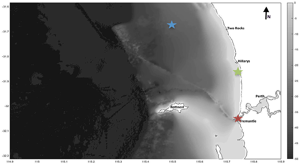
Figure 1. Study site with bathymetry. Offshore (blue), nearshore (green) and estuarine (red) areas are highlighted as stars.
Leeuwin Current in the Offshore
The Leeuwin Current (LC) presents one of the key drivers of local oceanography and climatology in Western Australia. It is an anomalous eastern boundary current that flows poleward against prevailing equatorward winds (Godfrey and Ridgway, 1985). The LC is driven by an alongshore geopotential gradient created by warm, nutrient-poor Pacific Ocean waters spilling into the Indian Ocean with the Indonesian Through-flow (ITF) (Pearce and Phillips, 1988; Fieux et al., 2005). While most of the ITF contributes to the westward flowing Indian Ocean Equatorial current, some of it flows into the Holloway current along the North West shelf of Australia and extends further south where it contributes to the LC (Pearce and Phillips, 1988; Yit Sen Bull and van Sebille, 2016). Seasonal variability of the LC creates strongest transport during the austral winter months, as opposing winds weaken (Godfrey and Ridgway, 1985; Feng et al., 2003). A peak in LC strength within the study area is observed from May to June each year, when the alongshore pressure gradient peaks (Morrow and Birol, 1998). While interannual peaks are driven by Pacific sea level variations, Ridgway and Godfrey (2015) have proposed a monsoonal sea level pulse as the driver of seasonal variations. This post-monsoon pulse explains maximum flow in the South West of Western Australia from May to June (Feng et al., 2003). Transport of international plastic pollutants to the area is facilitated through entrainment of Indian Ocean surface waters and the ITF, which extends into the Holloway and then Leeuwin Current, capable of transporting water down the coast from Asia (Meyers et al., 1995; Pattiaratchi and Woo, 2009). ITF waters are hereby modeled to make up the highest proportion of water transported in the LC (Yit Sen Bull and van Sebille, 2016). Importantly, the three countries with the highest estimated influx of mismanaged plastic waste to the ocean—namely China, Indonesia and the Philippines—are directly connected to Western Australia by these surface currents (Jambeck et al., 2015). Therefore, it is hypothesized that the highest concentrations of plastic pollution in the offshore will occur during strongest Leeuwin current flow in May.
Rainfall and Estuarine-sourced Debris
The Perth metropolitan coast is a micro-tidal environment with a diurnal tide of approximately 0.6 m (Ruiz-Montoya and Lowe, 2014). The Swan River estuary is a predominantly tidally driven, seasonally reversing estuary. Over the past decades, the area has been experiencing increasingly long droughts during the summer months (Gallant et al., 2013), with the bulk of rainfall occurring in the austral winter (Smith et al., 2000). Recent decades have seen a decrease in rainfall in addition to increasingly concentrated rainfall patterns during the early austral winter (May–July), as opposed to an even spread into the later winter months (August–October) (Smith et al., 2000). With a sampling protocol that targets Swan River effluent during ebb tides, it is expected that the highest amounts of estuarine-sourced pollution will be recorded directly after concentrated rainfall events during the early winter months, from May through to July.
Coastal Current Dominating the Nearshore
The coastal current (CC) is a northward alongshore current flowing strongest during the austral summer when southerly winds are strongest (Ruiz-Montoya and Lowe, 2014). It has been suggested to be an extension of the Capes Current flowing between Cape Leeuwin and Cape Naturaliste in the southwest of Western Australia (Pearce and Pattiaratchi, 1999), The nearshore circulation pattern of the coastal current in PMW during summer is highly variable and responds quickly to changes in wind, but is mostly driven northward by the dominant southerly sea breeze (Pattiaratchi et al., 1997; Ruiz-Montoya and Lowe, 2014). In the presence of predominantly southerly winds concentrations in the nearshore are therefore expected to be highest after periods of rain, as estuarine outfall can be accumulated against the shore, with the LC creating a boundary preventing offshore transport of plastic particles.
Data Collection
All plastic sampled was collected using a manta net (1 × 0.17 m, 333 micron mesh), designed and manufactured by Oceans Instruments, San Diego (Brown and Cheng, 1981; Goldstein et al., 2013; Reisser et al., 2013). One station in each of the three areas of interest was sampled on four occasions during the study period (Table 1). At each station the net was towed through the sea-surface interface in three consecutive replicate tows of 15 min (NOAA, 2015). All collected material was transferred from the cod-ends of the manta net to a transfer container (Reisser et al., 2013). The net and cod-end were carefully rinsed and plastics refloated in seawater within it. The transfer containers were then immediately and thoroughly examined visually for plastic pieces, placed into a graduated dish with forceps, individually counted, and transported to the lab in vials (similar procedures utilized by Morét-Ferguson et al., 2010; Cózar et al., 2014). Sampling was not conducted during high wind conditions, due to potential dangers of instrument deployment in rough seas and rapid decline in plastic detectability in the surface layer at high wind speeds (Kukulka et al., 2012; Reisser et al., 2014). Wind speed and tides were consulted in fieldwork planning and recorded throughout sampling. Planning ensured sampling of the estuarine sites occurred only during ebb tides, when flotsam is exiting out the estuary, and that dangerous seas were avoided. Rainfall, wind speed, and wind direction time-series data was obtained from the Bureau of Meteorology (2015), from measurements taken on Rottnest Island in 30-min intervals. Significant wave height data is based on a localized surf forecast by Wandres (2015) based on the ERA –Interim model reanalysis (Dee et al., 2011).
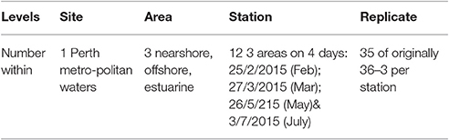
Table 1. Reference table for levels of sampling procedure.
Data Recording
To estimate surface concentrations at all stations the total numbers of plastics were standardized to pieces per km2 (Law et al., 2010). Surface area was calculated using tow length × net width for each replicate tow. The concentrations are reported as a mean in pieces/km2 and presented as an averaged value from the replicate tows at each station and their standard deviation (Reisser et al., 2013; NOAA, 2015). Tow length was measured with a General Oceanics analog flow meter, fixed inside the manta net frame (Brown and Cheng, 1981; Goldstein et al., 2013), and cross-validated with GPS measurements of the sampled transects (Reisser et al., 2013). Whilst Kukulka et al. (2012) have demonstrated that wind speeds can have a significant effect on the detectability of plastics in the surface layer, and proposed a one-dimensional column model for estimation of wind integrated plastic surface concentrations, this model was not used in this study. Since the maximum depth at any sampling site was 34 m, a well-mixed water column was expected, which was confirmed in the detection of a small number of non-buoyant plastics during sampling.
After sampling all plastics were air dried at room temperature for at least 24 h. All plastics were measured along their maximum length and recorded to the nearest 0.5 mm using a millimeter ruler. For plastics that were larger than 30 cm a measuring tape was used. Particles between the minimum limit of detection, 0.33 mm, and 1 mm were conservatively recorded as 0.8 mm to allow for statistical analysis of continuous data (Eriksen et al., 2014). The collected plastics were then categorized into several types—namely hard/sheet, soft/film, line, styrofoam, rubber, cellulose, and microbeads—and their color recorded. Such characterizations are important for geographic and temporal comparisons (Shaw and Day, 1994; Morét-Ferguson et al., 2010). Yet, no uniform characterization approach exists. All common categories identified in a recent review of the relevant literature were used, with the exception of preproduction pellets, since none were found in the study site (Hidalgo-Ruz et al., 2012). Further, infrared Raman spectroscopy was applied to a randomly selected, representative subsample from all areas and replicate tows (total n = 116) (Allen et al., 1999; Cózar et al., 2014). For Raman spectroscopy the non-destructive confocal Raman instrument WiTec Alpha 300 was used. The instrument was pre-calibrated with a silicon wafer (Murray and Cowie, 2011), and spectra recorded under a 200 μm scan stage with 532 nm excitation lengths. Raman spectrometry served to confirm that all plastics collected were in fact synthetic polymers (Allen et al., 1999), since visual analysis alone might be prone to human errors and accuracy of results otherwise questionable (Hidalgo-Ruz et al., 2012; Lenz et al., 2015).
Statistical Analyses
Preliminary plotting of data obtained for both concentrations and sizes showed a highly skewed distribution and heteroskedasticity in model residuals even after log transformations. As a result, non-parametric analyses were performed in the RStudio package. To test for significant differences in plastic concentrations between areas and over time, firstly, a nonparametric Kruskal-Wallis analysis of variance (KW-ANOVA) was used (Kruskal and Wallis, 1952). The KW-ANOVA determines if at least one of the areas or months is statistically different, without elucidating which ones specifically differ (Kruskal and Wallis, 1952; Dunn, 1964). After establishing if at least one population was significantly different, a post-hoc Dunn's (1964) rank sum test was run to see where exactly the differences occurred (Dinno, 2015). The Dunn's test is a convenient joint ranking method, applicable to test the null hypothesis that concentrations and sizes are identically distributed in populations—or in this case areas and months (Sherman, 1965). Significant p-values after the Dunn's test show which exact areas and months differ. To determine variations in characteristics between areas all recorded data was manually transformed into counts in Microsoft Excel™. Chi-square tests were used to determine if the proportion of types and colors varied between areas overall for comparison with other studies. To analyze differences in the characteristics between areas and size groups, data were visualized using non-metric multidimensional scaling (nMDS) based on Bray-Curtis dissimilarity in R (Oksanen et al., 2015). Bray Curtis is stable to the many zeros present in count data sets. Despite the fact that some counts were very high, no transformations were applied to the data, since our questions were mainly quantitative and would not merit from emphasizing less common types and colors. To test if the differences in characteristics were statistically significant between areas a permutational analysis of variance (PERMANOVA with 999 permutations) was applied with the effects of area, month, rainfall, wind speed and wind direction as independent and random factors. Pairwise comparisons of random factors are rarely logical in PERMANOVA approaches and therefore no tests were performed for interactions in this analysis (Anderson et al., 2008).
Results
Concentrations
A total of 716 pieces of plastic were found. Material was found at all sites during all sampling times, and only one replicate tow produced no plastic fragments. Importantly, all plastics from the subsample (n = 116) were confirmed to be plastics by Raman spectrometry, giving confidence in the overall concentration estimates. The most common type of plastic overall was fishing line (38%), especially in the nearshore and estuarine areas, closely followed by hard plastic fragments (35%), which dominated in the offshore. Primary microplastics, all in the form of cosmetic microbeads, made up 6% (n = 42) of the overall sample and were most common in the nearshore area, but present in all areas. The highest concentrations of plastic pollution were detected in the nearshore environment during sampling in early July, and in the estuary and offshore in late May (Table 2). These concentrations confirmed hypotheses about predictable high concentrations in accordance with their respective drivers. In the offshore the highest concentration is in line with seasonally increased Leeuwin current flow. In May plastics were sampled within days of the first major rain event (Figure 2). This is reflected in the high concentration of estuarine plastics. Yet the nearshore showed much higher concentrations in early July than directly after the rainfall event in May.
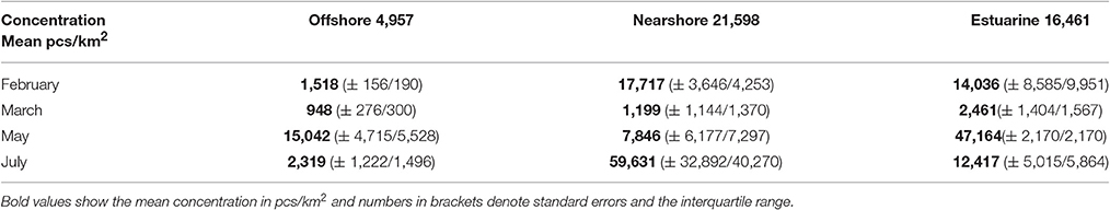
Table 2. Mean plastic pollution concentrations in pieces/km2 in PMW.
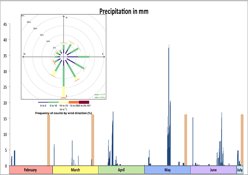
Figure 2. Histogram of precipitation in mm (blue bars) over the study period (Source: Bureau of Meteorology, 2015). Sampling days marked by orange bars and inset is a wind rose of wind speeds and direction. For the wind rose colors denote: blue = 0–5, green = 5–10, yellow 10–15, orange 15–20, red 20–24.17 m s−1 (R openair package: Carslaw and Ropkins, 2012).
Unexpectedly low concentrations for all areas were detected in March. Consecutive days of offshore winds were recorded prior to sampling in March. In some cases, standard deviations and interquartile ranges were found to be nearly as high as concentrations; evidence of immense spatial variability even between replicate tows (distance ~ 1 nm).
The KWANOVA results showed a significant result for the interaction of area, month and rainfall in predicting concentrations (p = 0.0026). Spatial Dunn's test results show that both the estuary and the nearshore where significantly different form the offshore, but not from each other (Table 3). Temporal comparison of concentrations by month showed that March was significantly different form all other months and overpowered other significant differences. Detailed spatiotemporal results show that the offshore differed from all other months in May, and the estuarine only differed between March and May (Table 4). For the nearshore, significant differences were recorded for March and July compared to other months.
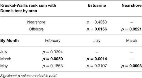
Table 3. Dunn's test results for differences in concentration by area and month.
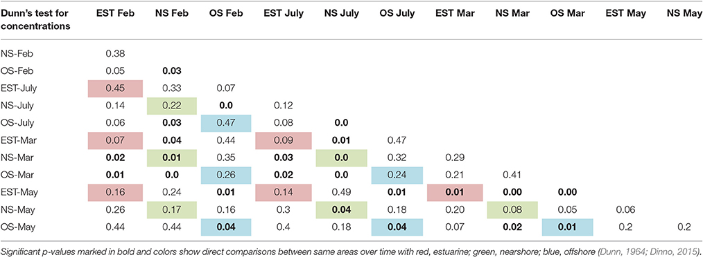
Table 4. Post-hoc Dunn's test of concentrations.
Plastic Size and Characteristics
KWANOVA identified a highly significant interaction of area, time and rainfall (p < 0.005) in determining plastic particle size. Dunn's test showed that size differed between all areas, and between but not within austral summer and winter months (Table 5). Offshore plastics were smallest and least variable, while estuarine had the largest fragments and interquartile ranges. Histograms of sizes reflect this and show the increased frequency of counts for larger sizes during May and July (Figures 3, 4). Plastics in the smallest size categories were the most common in all areas and at all times. Sizes for the histograms presented were capped at 20 mm to be comparable to other studies (Hidalgo-Ruz et al., 2012), and to minimize one tailed skew.
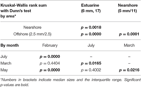
Table 5. Dunn's test results for spatial and temporal differences in size.
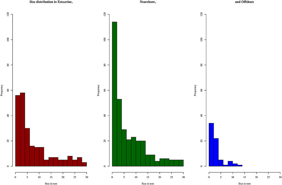
Figure 3. Histogram of sizes distribution between areas.
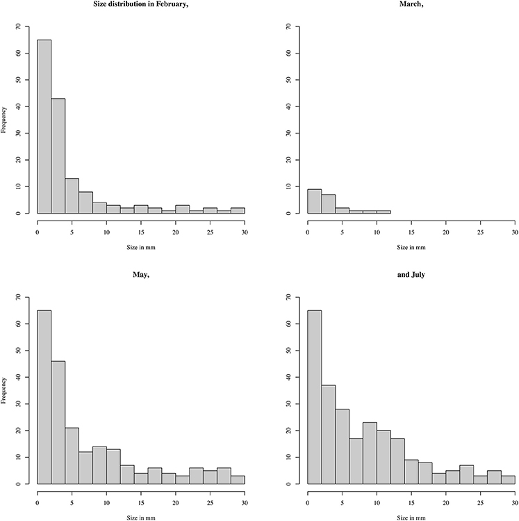
Figure 4. Histogram of sizes over the duration of the study.
Using chi-square tests showed a highly significant difference for the proportions of type (levels = 7, p < 0.005) and color (levels 13, p = 0.013) for the offshore from other areas, but no significant difference between the estuarine and nearshore areas. Offshore samples were dominated by hard plastics (fragments and microbeads adding to 70%) and estuarine and nearshore were predominantly fishing line (38 and 44% respectively, Figure 5). In terms of color, offshore plastics were predominantly white and clear in color (44 and 17%, Figure 6). In contrast, plastics from the nearshore and estuary showed a more heterogeneous array of colors with white making up only 25% in both. This difference can also be seen in the clustering of offshore samples in the nMDS that is distinct from the wide spread of nearshore and estuarine scaling (Figures 7, 8). For the offshore, a deviation from the otherwise tight cluster can be seen in May. This indicates that along with higher concentrations reported earlier a wider variety of plastics types and colors are arriving with increased LC flow. PERMANOVA results show that main effects of area, month, rainfall and wind direction were significant in driving differences for type (p = 0.039, 0.002, 0.001, 0.003 respectively) and color (p = 0.002, 0.002, 0.001, 0.006 respectively), but wind speed was not (p type = 0.362, p color = 0.313).
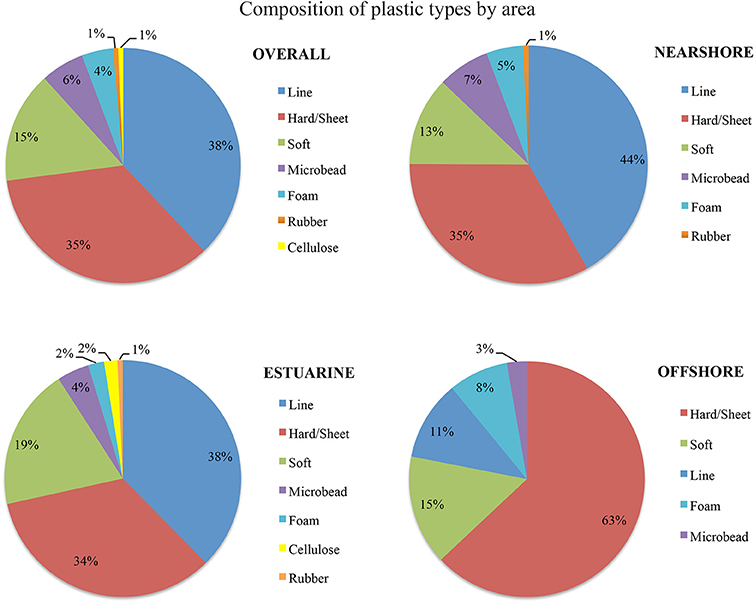
Figure 5. Composition of plastic types recorded overall and between areas.
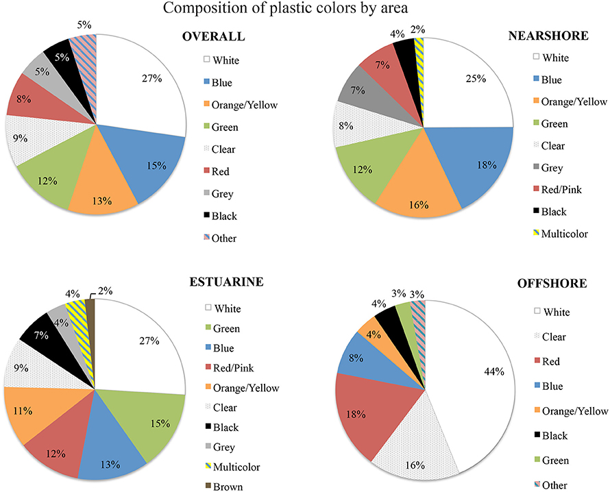
Figure 6. Composition of plastic colors recorded overall and between areas.
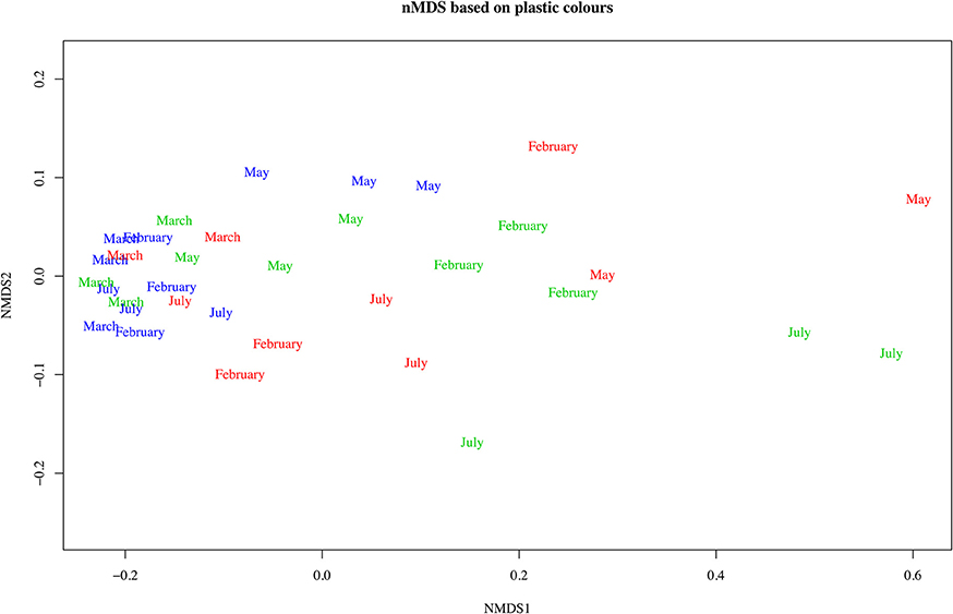
Figure 7. Non-metric multidimensional scaling of Bray Curtis dissimilarity matrix computed from type counts for Perth metropolitan plastics. Color of text indicates the area of interest: blue, offshore; green, nearshore; red, estuarine.
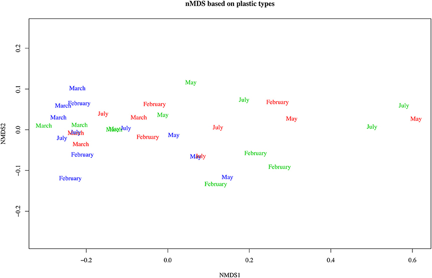
Figure 8. Non-metric multidimensional scaling of Bray-Curtis dissimilarity matrix computed from color counts for Perth metropolitan plastics. Color of text indicates the area of interest: blue, offshore; green, nearshore; red, estuarine.
Discussion
Concentrations and Drivers of Variability
Australia has one of the largest exclusive economic zones in the world and 59,700 km of coastline, with a vast majority of the population living in coastal areas. Prior to this study, sampling of buoyant plastics in Australian waters had been limited to approximately 60 sampling locations all around the continent (Reisser et al., 2013; Cózar et al., 2014). This study shows that concentrations of plastic pollution varied both between areas of interest and over time. Particularly the offshore area diverged widely from the estuarine and nearshore samples. The mean offshore concentration of 4,957 pieces per km−2 is comparable to previously recorded concentrations of 4256.4 pieces per km−2 in waters around the Australian continent by Reisser et al. (2013). However, temporal comparison showed that this figure could increase by an order of magnitude with increased LC flow (Figure 2). This increased figure is still substantially lower than high concentrations reported in subtropical gyres of up to 3.309 × 10⁴ and 5.8 × 10⁵ pieces/km−2 in the eastern North Pacific and North Atlantic respectively (Law et al., 2010, 2014). Yet, PMW average concentrations are higher than in other coastal seas, such as the Caribbean Sea (1,414 ± 112) or the Gulf of Maine (1,534 ± 200) (Law et al., 2010), and historical records from the Sargasso Sea (Carpenter and Smith, 1972), but lower than in comparable coastal current systems such as the Kuroshio Current (Yamashita and Tanimura, 2007). While quantification of plastics per unit of area is the most commonly used (Hidalgo-Ruz et al., 2012), differential recording of plastic concentrations as pieces per volume or in weight limits further direct comparisons (Gilfillan et al., 2009; Doyle et al., 2011).
The statistical test results showed that temporal and spatial variation could be mutually confounding, as evident in significant interaction effects for both concentrations and size. Law et al. (2014) have previously pointed this out. However by using detailed pairwise comparisons a clearer picture could be gained in this study. The confounding effects of offshore winds in March could thus be recognized without statistically overwhelming important differences between other months and areas. Previous studies have tried to navigate variability by comparing samples within spatial bins and over multiple time frames (Gilfillan et al., 2009; Morét-Ferguson et al., 2010), or spatial scales (Doyle et al., 2011; Goldstein et al., 2013), but without clearly addressing variability of physical drivers. This study had added the understanding that a focus on physical drivers—which are highly variable in space and time—rather than one large-scale feature (coastlines or gyres), can inform on the particular dynamics of interest. Furthermore, using areas for comparison rather than distance based approaches may effectively cut down sample size requirements for spatiotemporal analyses (Goldstein et al., 2013). A continuation and extension of this research design is recommended to address the utility of this approach for multi-year and decadal changes, since the sampling for this study was limited by time constraints. In those areas were historical data of plastic pollution exists measured concentrations can be coupled with historical field measurements or numerical models of physical drivers to select informed areas for comparison (Thompson et al., 2004; Gilfillan et al., 2009; Morét-Ferguson et al., 2010). This way more information may be gleaned about and from variability, which was previously not easily explained in multi-decadal or multi-year analyses.
Some preliminary predictions can be discussed to inform future research from the observed short-term variability of areas in accordance with their physical drivers. This study found that offshore microplastics, introduced to the study site with the Leeuwin current, increased with strength of flow in May. Both the ITC and Australian Monsoon driving LC variability are susceptible to changes based on El Niño Southern Oscillation (ENSO) (Pearce and Phillips, 1988; Jourdain et al., 2013). Therefore, concentrations may be significantly higher during non-ENSO years and La Nina episodes (Pearce and Phillips, 1988). With climate change driven rises in sea surface temperatures, the geostrophic Leeuwin flow is likely to increase, regardless of ENSO, and may bring with it higher concentrations of plastic fragments to local waters. This would present an additional stressor to the Western Australian marine environment that suffers significant heat stresses as a result of strong La Nina periods (Pearce et al., 2011). On the other hand, previous research has shown that ENSO periods lead to a weakening of large-scale subtropical gyre circulation and results in less concentrated debris within the center (Martinez et al., 2009). Therefore, an alternative theory would be that debris from the inner Indian Ocean subtropical gyre, spreading across the basin during El Niño episodes, might become more easily entrained into the Leeuwin current through geostrophic flow. These are some questions that can be answered through ongoing research and field sampling in the future.
Rain-induced estuarine and coastal concentrations were very high in comparison to other coastal areas, such as the Gulf of Maine and the Caribbean (Table 2; Law et al., 2010). A positive finding is that the dynamics of effluent from the estuary and delayed concentration along the shore was highly predictable and concentrated in time and space. This predictability may create opportunities for cost-effective cleanup initiatives. Technologies for pelagic plastic cleanups are currently being developed and trialed (Slat, 2015). Continuous study and improved understanding of the dynamics of estuarine and nearshore pollution can inform potential installations of clean up arrays. Well-timed, short-term installations could perceivably minimize impacts on marine life and shipping whilst reducing maintenance costs. Allan and Haylock (1993) found a strong relationship between declining rainfall along the Southwestern Australian coast and sea level pressure. With reduced and more concentrated rainfall patterns, pollution retention may become an increasing problem in the Swan River Estuary in decades to come.
Size of Plastic Fragments in PMW
As expected, the smallest fragments of plastic products were found in the offshore, and the largest in the estuary. Therefore, results presented here support the assumption that smaller plastics are “older” or have had longer residence times at sea, as long as the differentiation between SMPs and PMPs is made. The ubiquity of plastics in the smallest size category across all areas at all times raises concern about toxic effects of local pollution. The amplified hydrophilic potential of smaller fragments in the local environment may make for an underestimated impact on marine biota, when concentrations alone are considered. This study showed that small fragments are present, and likely moving in and out of the tide dominated Swan Estuary, where a large harbor is located (Figure 1). The most recent report by the Swan River Trust shows that environmental targets are not being met and water quality is deteriorating (Swan River Trust, 2016). If this trend continues, threat to marine and estuarine biota through plastic ingestion may be significant and increasing. As such monitoring of plastic pollution and additional studies on pollutant loads are recommended (Murray and Cowie, 2011; Rochman, 2015).
The skewedness of size distributions also suggests that a substantial amount of material below the manta net's limit of detection (333 micron) is present in local waters. The strong sea breeze in the area increases incident wave energy (Pattiaratchi et al., 1997). This may result in rapid mechanical breakdown of plastic particles trapped in the nearshore. New methods for the quantification of smaller size ranges are being developed and tested (for example: Enders et al., 2015). Further testing of such methods and comparative analysis with more standard approaches (such as presented here) is warranted to determine a viable method for the quantification of nano-plastics and their chemical loads and toxicity.
Types and Colors of Plastic Fragments
A significant difference between the types of plastics found in nearshore and estuary vs. the offshore gives some indication about local discard practices, which can be addressed through educational initiatives. The large amount of fishing line found exiting the estuary and in the nearshore points at substantial pollution from recreational fishing activities. Implementing initiatives to address this source and monitoring future trends can become one form of Key Performance Indicator for local environmental management. Offshore samples in PMW, on the other hand, seem to have a comparably more “oceanic signature.” They are similar in type and colors to what has previously been recorded in deeper waters around Australia, the North Pacific and the North Atlantic: Reisser et al. (2013) reported 75% of plastics found around Australia were hard fragments, while Shaw and Day (1994) and Morét-Ferguson et al. (2010) reported 60–90% for the Pacific, and 50–90% for the Atlantic respectively. Furthermore, white or clear plastics made up 85% of fragments in Australian waters and 75% in the North Pacific Ocean. Previous studies have shown that these characteristics can inform on changes over time and between size classes (Shaw and Day, 1994; Vlietstra and Parga, 2002; Morét-Ferguson et al., 2010). Results presented here indicated some change occurring in the offshore with increased LC flow even over the limited time frame of this pilot study. Therefore, continuing to record this information is encouraged, for detailed detection of change in the future, to firstly better understand predator selectivity, and secondly enable comparisons with other studies globally.
Conclusions
One of the major finds of this case study is that statistically significant differences in concentrations of plastic pollution between areas over the short-term duration of the project were largely predictable. Where oceanic drivers were not predictive of the resulting concentrations, deviations could be explained through recorded climatic conditions, in this case wind direction. On one hand, this raises questions about the feasibility of extrapolation from single time-frame measurements as being representative of a full year for inter-annual comparison. On the other hand, it provides some insights to sources and dynamics of interest in similar environments globally. This case study provides an approach that may be more reliable in detecting trends and changes at multi-year or multi-decadal scales in the future. Using pairwise comparisons of previously defined areas may also yield better results in future studies, due to a reduced sample size needed for comparison and greater focus on oceanographic and climatic data explaining variability. This study adds to the very limited body of information for pelagic plastic pollution in Australian waters and compares local concentrations and characteristics with global data. A number of preliminary predictions were made, which will need to be tested in future research. In terms of findings that can be implemented for mitigation, the data shows that the majority of pollution is from local sources and dominated by fishing line in small size fractions. This indicates a clear fishing-related primary source of pollution. While further research will be invaluable in directing management recommendations to tackle this pervasive environmental problem over time, addressing the specific sources and behaviors leading to of plastic pollution is an important first step. This shows the benefits of qualitative analyses of plastic characteristics, which have the potential inform sources, rather than purely quantitative studies focusing on the state of pollution.
Author Contributions
All authors listed, have made substantial, direct and intellectual contribution to the work, and approved it for publication.
Conflict of Interest Statement
The authors declare that the research was conducted in the absence of any commercial or financial relationships that could be construed as a potential conflict of interest.
Acknowledgments
This work was funded by the Australian Integrated Marine Observing System's (IMOS) Australian National Facility for Ocean Gliders (ANFOG) at The University of Western Australia and the PADI Foundation (grant number CGA# 11311), CA. The authors acknowledge the facilities, and the scientific and technical assistance of the Australian Microscopy & Microanalysis Research Facility at the Centre for Microscopy, Characterisation & Analysis (CMCA), The University of Western Australia, a facility funded by the University, State and Commonwealth Governments. We would like to thank Dennis Stanley of ANFOG, and L. Kirilak & T. Becker of CMCA in particular for their technical assistance and recommendations.
References
Allan, R. J., and Haylock, M. R. (1993). Circulation features associated with the winter rainfall decrease in southwestern Australia. J. Clim. 6, 1356–1367.
Allen, V., Kalivas, J. H., and Rodriguez, R. G. (1999). Post-consumer plastic identification using Raman spectroscopy. Appl. Spectrosc. 53, 672–681.
Anderson, M., Gorley, R., and Clarke, K. (2008). PERMANOVA1 for PRIMER: Guide to Software and Statistical Methods. Plymouth: PRIMER-E.
Andrady, A. L. (2011). Microplastics in the marine environment. Mar. Pollut. Bull. 62, 1596–1605. doi: 10.1016/j.marpolbul.2011.05.030
Avio, C. G., Gorbi, S., Milan, M., Benedetti, M., Fattorini, D., d'Errico, G., et al. (2015). Pollutants bioavailability and toxicological risk from microplastics to marine mussels. Environ. Pollut. 198, 211–222. doi: 10.1016/j.envpol.2014.12.021
Barnes, D. K., Galgani, F., Thompson, R. C., and Barlaz, M. (2009). Accumulation and fragmentation of plastic debris in global environments. Philos. Trans. R. Soc. B. Biol. Sci. 364, 1985–1998. doi: 10.1098/rstb.2008.0205
Brown, D., and Cheng, L. (1981). New net for sampling the ocean surface. Mar. Ecol. Prog. Ser. 5, 224–227.
Bureau of Meteorology (2015). Latest Weather Observations for Rottnest Island. Canberra, ACT: Bureau of Meteorology, Commonwealth of Australia.
Carpenter, E. J., and Smith, K. (1972). Plastics on the Sargasso Sea surface. Science 175, 1240–1241.
Carslaw, D. C., and Ropkins, K. (2012). Openair—an R package for air quality data analysis. Environ. Model Softw. 27, 52–61. doi: 10.1016/j.envsoft.2011.09.008
Carson, H. S., Lamson, M. R., Nakashima, D., Toloumu, D., Hafner, J., Maximenko, N., et al. (2013). Tracking the sources and sinks of local marine debris in Hawai‘i. Mar. Environ. Res. 84, 76–83. doi: 10.1016/j.marenvres.2012.12.002
Cole, M., Lindeque, P., Halsband, C., and Galloway, T. S. (2011). Microplastics as contaminants in the marine environment: a review. Mar. Pollut. Bull. 62, 2588–2597. doi: 10.1016/j.marpolbul.2011.09.025
Corcoran, P. L., Biesinger, M. C., and Grifi, M. (2009). Plastics and beaches: a degrading relationship. Mar. Pollut. Bull. 58, 80–84. doi: 10.1016/j.marpolbul.2008.08.022
Cózar, A., Echevarría, F., González-Gordillo, J. I., Irigoien, X., Úbeda, B., Hernández-León, S., et al. (2014). Plastic debris in the open ocean. Proc. Natl. Acad. Sci. U.S.A. 111, 10239–10244. doi: 10.1073/pnas.1314705111
Dee, D., Uppala, S., Simmons, A., Berrisford, P., Poli, P., Kobayashi, S., et al. (2011). The ERA-Interim reanalysis: configuration and performance of the data assimilation system. Q. J. R. Meteorol. Soc. 137, 553–597. doi: 10.1002/qj.828
Derraik, J. G. B. (2002). The pollution of the marine environment by plastic debris: a review. Mar. Pollut. Bull. 44, 842–852. doi: 10.1016/S0025-326X(02)00220-5
Dinno, A. (2015). dunn.test: Dunn's Test of Multiple Comparisons Using Rank Sums, R Package Version 1.3. Available online at: http://CRAN.R-project.org/package=dunn.test
do Sul, J. A. I., and Costa, M. F. (2014). The present and future of microplastic pollution in the marine environment. Environ. Pollut. 185, 352–364. doi: 10.1016/j.envpol.2013.10.036
Doyle, M. J., Watson, W., Bowlin, N. M., and Sheavly, S. B. (2011). Plastic particles in coastal pelagic ecosystems of the Northeast Pacific ocean. Mar. Environ. Res. 71, 41–52. doi: 10.1016/j.marenvres.2010.10.001
Enders, K., Lenz, R., Stedmon, C. A., and Nielsen, T. G. (2015). Abundance, size and polymer composition of marine microplastics ≥ 10μm in the Atlantic Ocean and their modelled vertical distribution. Mar. Pollut. Bull. 100, 70–81. doi: 10.1016/j.marpolbul.2015.09.027
Eriksen, M., Lebreton, L. C., Carson, H. S., Thiel, M., Moore, C. J., Borerro, J. C., et al. (2014). Plastic pollution in the World's Oceans: more than 5 trillion plastic pieces weighing over 250,000 tons Afloat at Sea. PLoS ONE 9:e111913. doi: 10.1371/journal.pone.0111913
Eriksen, M., Maximenko, N., Thiel, M., Cummins, A., Lattin, G., Wilson, S., et al. (2013). Plastic pollution in the South Pacific subtropical gyre. Mar. Pollut. Bull. 68, 71–76. doi: 10.1016/j.marpolbul.2012.12.021
Erren, T. C., Groß, J. V., Steffany, F., and Meyer-Rochow, V. B. (2015). “Plastic ocean”: what about cancer? Environ. Pollut. 207, 436–437. doi: 10.1016/j.envpol.2015.05.025
Feng, M., Meyers, G., Pearce, A., and Wijffels, S. (2003). Annual and interannual variations of the Leeuwin current at 32 S. J. Geophys. Res. Oceans 108:3355. doi: 10.1029/2002JC001763
Fieux, M., Molcard, R., and Morrow, R. (2005). Water properties and transport of the Leeuwin current and eddies off Western Australia. Deep Sea Res. Part I 52, 1617–1635. doi: 10.1016/j.dsr.2005.03.013
Gallant, A. J. E., Reeder, M. J., Risbey, J. S., and Hennessy, K. J. (2013). The characteristics of seasonal-scale droughts in Australia, 1911–2009. Int. J. Climatol. 33, 1658–1672. doi: 10.1002/joc.3540
Gilfillan, L. R., Ohman, M. D., Doyle, M. J., and Watson, W. (2009). Occurrence of plastic micro-debris in the southern California current system. Cal. Coop. Ocean. Fish. 50, 123–133. Available online at: http://137.110.142.7/publications/CR/2009/2009Gilf.pdf
Godfrey, J., and Ridgway, K. (1985). The large-scale environment of the poleward-flowing Leeuwin current, Western Australia: longshore steric height gradients, wind stresses and geostrophic flow. J. Phys. Oceanogr. 15, 481–495. doi: 10.1175/1520-0485(1985)015<0481:TLSEOT>2.0.CO;2
Goldstein, M. C., Titmus, A. J., and Ford, M. (2013). Scales of spatial heterogeneity of plastic marine debris in the northeast Pacific Ocean. PLoS ONE 8:e80020. doi: 10.1371/journal.pone.0080020
Gregory, M. R. (2009). Environmental implications of plastic debris in marine settings—entanglement, ingestion, smothering, hangers-on, hitch-hiking and alien invasions. Philos. Trans. R. Soc. B. Biol. Sci. 364, 2013–2025. doi: 10.1098/rstb.2008.0265
Hidalgo-Ruz, V., Gutow, L., Thompson, R. C., and Thiel, M. (2012). Microplastics in the marine environment: a review of the methods used for identification and quantification. Environ. Sci. Technol. 46, 3060–3075. doi: 10.1021/es2031505
Isobe, A., Uchida, K., Tokai, T., and Iwasaki, S. (2015). East Asian seas: a hot spot of pelagic microplastics. Mar. Pollut. Bull. 101, 618–623. doi: 10.1016/j.marpolbul.2015.10.042
Jambeck, J. R., Geyer, R., Wilcox, C., Siegler, T. R., Perryman, M., Andrady, A., et al. (2015). Plastic waste inputs from land into the ocean. Science 347, 768–771. doi: 10.1126/science.1260352
Jourdain, N. C., Gupta, A. S., Taschetto, A. S., Ummenhofer, C. C., Moise, A. F., and Ashok, K. (2013). The Indo-Australian monsoon and its relationship to ENSO and IOD in reanalysis data and the CMIP3/CMIP5 simulations. Clim. Dyn. 41, 3073–3102. doi: 10.1007/s00382-013-1676-1
Kruskal, W. H., and Wallis, W. A. (1952). Use of ranks in one-criterion variance analysis. J. Am. Stat. Assoc. 47, 583–621.
Kubota, M. (1994). A mechanism for the accumulation of floating marine debris north of Hawaii. J. Phys. Oceanogr. 24, 1059–1064.
Kukulka, T., Proskurowski, G., Morét-Ferguson, S., Meyer, D. W., and Law, K. L. (2012). The effect of wind mixing on the vertical distribution of buoyant plastic debris. Geophys. Res. Lett. 39:L07601. doi: 10.1029/2012GL051116
Law, K. L., Morét-Ferguson, S. E., Goodwin, D. S., Zettler, E. R., DeForce, E., Kukulka, T., et al. (2014). Distribution of surface plastic debris in the Eastern Pacific Ocean from an 11-year data set. Environ. Sci. Technol. 48, 4732–4738. doi: 10.1021/es4053076
Law, K. L., Morét-Ferguson, S., Maximenko, N. A., Proskurowski, G., Peacock, E. E., Hafner, J., et al. (2010). Plastic accumulation in the North Atlantic subtropical gyre. Science 329, 1185–1188. doi: 10.1126/science.1192321
Lenz, R., Enders, K., Stedmon, C. A., Mackenzie, D. M. A., and Nielsen, T. G. (2015). A critical assessment of visual identification of marine microplastic using Raman spectroscopy for analysis improvement. Mar. Pollut. Bull. 100, 82–91. doi: 10.1016/j.marpolbul.2015.09.026
Martinez, E., Maamaatuaiahutapu, K., and Taillandier, V. (2009). Floating marine debris surface drift: convergence and accumulation toward the South Pacific subtropical gyre. Mar. Pollut. Bull. 58, 1347–1355. doi: 10.1016/j.marpolbul.2009.04.022
Meyers, G., Bailey, R., and Worby, A. (1995). Geostrophic transport of Indonesian throughflow. Deep Sea Res. Part I. 42, 1163–1174.
Morét-Ferguson, S., Law, K. L., Proskurowski, G., Murphy, E. K., Peacock, E. E., and Reddy, C. M. (2010). The size, mass, and composition of plastic debris in the western North Atlantic Ocean. Mar. Pollut. Bull. 60, 1873–1878. doi: 10.1016/j.marpolbul.2010.07.020
Morrow, R., and Birol, F. (1998). Variability in the southeast Indian Ocean from altimetry: forcing mechanisms for the Leeuwin current. J. Geophys. Res. Oceans 103, 18529–18544. doi: 10.1029/98JC00783
Murray, F., and Cowie, P. R. (2011). Plastic contamination in the decapod crustacean Nephrops norvegicus (Linnaeus, 1758). Mar. Pollut. Bull. 62, 1207–1217. doi: 10.1016/j.marpolbul.2011.03.032
NOAA (2015). How to Do a Manta Tow. Available online at: https://swfsc.noaa.gov/textblock.aspx?Division=FRD&id=1342
Oksanen, J., Blanchet, F. G., Kindt, R., Legendre, P., Minchin, P. R., O'Hara, R. B., et al. (2015). vegan: Community Ecology Package, R package version 2.2-1. Available online at: http://CRAN.R-project.org/package=vegan
Pattiaratchi, C., Hegge, B., Gould, J., and Eliot, I. (1997). Impact of sea-breeze activity on nearshore and foreshore processes in southwestern Australia. Cont. Shelf Res. 17, 1539–1560. doi: 10.1016/S0278-4343(97)00016-2
Pattiaratchi, C., and Woo, M. (2009). The mean state of the Leeuwin current system between North West Cape and Cape Leeuwin. J. R. Soc. West. Aust. 92, 221–241. Available online at: http://www.rswa.org.au/publications/Journal/92(2)/ROY%20SOC%2092.2%20LEEUWIN%20221-241.pdf
Pearce, A., Lenanton, R., Jackson, G., Moore, J., Feng, M., and Gaughan, D. (2011). “The “Marine heat wave” off Western Australia during the summer of 2010/11,” in Fisheries Research Report No. 222. Department of Fisheries, (Western Australia, WA).
Pearce, A., and Pattiaratchi, C. (1999). The Capes Current: a summer countercurrent flowing past Cape Leeuwin and Cape Naturaliste, Western Australia. Cont. Shelf Res. 19, 401–420. doi: 10.1016/S0278-4343(98)00089-2
Pearce, A., and Phillips, B. (1988). ENSO events, the Leeuwin Current, and larval recruitment of the western rock lobster. J. du Conseil: ICES J. Mar. Sci. 45, 13–21. doi: 10.1093/icesjms/45.1.13
Pérez, J. M., Vilas, J. L., Laza, J. M., Arnáiz, S., Mijangos, F., Bilbao, E., et al. (2010). Effect of reprocessing and accelerated ageing on thermal and mechanical polycarbonate properties. J. Mater. Process. Technol. 210, 727–733. doi: 10.1016/j.jmatprotec.2009.12.009
Reisser, J., Shaw, J., Wilcox, C., Hardesty, B. D., Proietti, M., Thums, M., et al. (2013). Marine plastic pollution in waters around Australia: characteristics, concentrations, and pathways. PLoS ONE 8:e80466. doi: 10.1371/journal.pone.0080466
Reisser, J., Slat, B., Noble, K., du Plessis, K., Epp, M., Proietti, M., et al. (2014). The vertical distribution of buoyant plastics at sea. Biogeosci. Discuss. 11, 16207–16226. doi: 10.5194/bg-12-1249-2015
Ridgway, K., and Godfrey, J. (2015). The source of the Leeuwin Current seasonality. J. Geophys. Res. Oceans 120, 6843–6864. doi: 10.1002/2015JC011049
Rochman, C. M. (2015). “The complex mixture, fate and toxicity of chemicals associated with plastic debris in the marine environment,” in Marine Anthropogenic Litter, eds M. Bergmann, L. Gutow, and M. Klages (Cham: Springer International Publishing), 117–140. doi: 10.1007/978-3-319-16510-3
Rochman, C. M., Kurobe, T., Flores, I., and Teh, S. J. (2014). Early warning signs of endocrine disruption in adult fish from the ingestion of polyethylene with and without sorbed chemical pollutants from the marine environment. Sci. Total Environ. 493, 656–661. doi: 10.1016/j.scitotenv.2014.06.051
Ruiz-Montoya, L., and Lowe, R. (2014). Summer circulation dynamics within the Perth coastal waters of southwestern Australia. Cont. Shelf Res. 77, 81–95. doi: 10.1016/j.csr.2014.01.022
Schuyler, Q., Hardesty, B. D., Wilcox, C., and Townsend, K. (2012). To eat or not to eat? Debris selectivity by marine turtles. PLoS ONE 7:e40884. doi: 10.1371/journal.pone.0040884
Seltenrich, N. (2015). New link in the food chain? Marine plastic pollution and seafood safety. Environm. Health Perspect. 123:A34. doi: 10.1289/ehp.123-A34
Shaw, D. G., and Day, R. H. (1994). Colour-and form-dependent loss of plastic micro-debris from the North Pacific Ocean. Mar. Pollut. Bull. 28, 39–43.
Slat, B. (ed.). (2015). World's First Ocean Cleaning System to be Deployed in 2016. T.O.C. Team. Available online at: http://www.theoceancleanup.com/blog/show/item/worlds-first-ocean-cleaning-system-to-be-deployed-in-2016.html
Smith, I., McIntosh, P., Ansell, T., Reason, C., and McInnes, K. (2000). Southwest Western Australian winter rainfall and its association with Indian Ocean climate variability. Int. J. Climatol. 20, 1913–1930. doi: 10.1002/1097-0088(200012)20:15<1913::AID-JOC594>3.0
Swan River Trust (2016). Final Report 2015–2016, Government of Western Australia. Available online at: https://swanrivertrust.dpaw.wa.gov.au/images/documents/annual_reports/37714_Swan_River_Trust_Annual_Report_2015-16_k2c_FNL2small.pdf
Thiel, M., Hinojosa, I., Miranda, L., Pantoja, J., Rivadeneira, M., and Vásquez, N. (2013). Anthropogenic marine debris in the coastal environment: a multi-year comparison between coastal waters and local shores. Mar. Pollut. Bull. 71, 307–316. doi: 10.1016/j.marpolbul.2013.01.005
Thompson, R. C., Olsen, Y., Mitchell, R. P., Davis, A., Rowland, S. J., John, A. W. G., et al. (2004). Lost at Sea: where is all the plastic? Science 304, 838. doi: 10.1126/science.1094559
Vegter, A. C., Barletta, M., Beck, C., Borrero, J., Burton, H., Campbell, M., et al. (2014). Global research priorities to mitigate plastic pollution impacts on marine wildlife. Endanger. Species Res. 25, 225–247. doi: 10.3354/esr00623
Vlietstra, L. S., and Parga, J. A. (2002). Long-term changes in the type, but not amount, of ingested plastic particles in short-tailed shearwaters in the southeastern Bering Sea. Mar. Pollut. Bull. 44, 945–955. doi: 10.1016/S0025-326X(02)00130-3
Wandres, M. (2015). Perth surfing Forecast. Available online at: online: http://perthsurfing.com/
Yamashita, R., and Tanimura, A. (2007). Floating plastic in the Kuroshio current area, western North Pacific Ocean. Mar. Pollut. Bull. 54, 485–488. doi: 10.1016/j.marpolbul.2006.11.012
Keywords: plastic pollution, spatiotemporal variability, coastal oceanography, Western Australia, mitigation, fishing line
Citation: Hajbane S and Pattiaratchi CB (2017) Plastic Pollution Patterns in Offshore, Nearshore and Estuarine Waters: A Case Study from Perth, Western Australia. Front. Mar. Sci. 4:63. doi: 10.3389/fmars.2017.00063
Received: 30 November 2016; Accepted: 20 February 2017;
Published: 10 March 2017.
Edited by:
Francois Galgani, French Research Institute for Exploitation of the Sea, FranceReviewed by:
Sunwook Hong, Our Sea of East Asia Network, South KoreaNicolas Kalogerakis, Technical University of Crete, Greece
Copyright © 2017 Hajbane and Pattiaratchi. This is an open-access article distributed under the terms of the Creative Commons Attribution License (CC BY). The use, distribution or reproduction in other forums is permitted, provided the original author(s) or licensor are credited and that the original publication in this journal is cited, in accordance with accepted academic practice. No use, distribution or reproduction is permitted which does not comply with these terms.
*Correspondence: Sara Hajbane, sara.hajbane@gmail.com