Modeling What We Sample and Sampling What We Model: Challenges for Zooplankton Model Assessment
 Jason D. Everett1,2*
  Mark E. Baird3
  Pearse Buchanan4 Cathy Bulman3 Claire Davies3 Ryan Downie3
  Chris Griffiths4,5
  Ryan Heneghan6 Rudy J. Kloser3
  Leonardo Laiolo3,7
  Ana Lara-Lopez8 Hector Lozano-Montes9
  Richard J. Matear3 Felicity McEnnulty3
  Barbara Robson10 Wayne Rochester11 Jenny Skerratt3 James A. Smith1,2
  Joanna Strzelecki9 Iain M. Suthers1,2 Kerrie M. Swadling4,12
  Paul van Ruth13
  Anthony J. Richardson6,11
- 1Evolution and Ecology Research Centre, University of New South Wales, Sydney, NSW, Australia
- 2Sydney Institute of Marine Science, Sidney, NSW, Australia
- 3CSIRO Oceans and Atmosphere, Hobart, TAS, Australia
- 4Institute for Marine and Antarctic Studies, University of Tasmania, Hobart, TAS, Australia
- 5School of Mathematics and Statistics, University of Sheffield, Sheffield, UK
- 6Centre for Applications in Natural Resource Mathematics, School of Mathematics and Physics, University of Queensland, St. Lucia, QLD, Australia
- 7Plant Functional Biology and Climate Change Cluster, Faculty of Science, University of Technology Sydney, NSW, Australia
- 8Integrated Marine Observing System, University of Tasmania, Hobart, TAS, Australia
- 9CSIRO Oceans and Atmosphere, Floreat, WA, Australia
- 10CSIRO Land and Water, Canberra, ACT, Australia
- 11CSIRO Oceans and Atmosphere, Dutton Park, QLD, Australia
- 12Antarctic Climate & Ecosystems CRC, Hobart, TAS, Australia
- 13South Australian Research and Development Institute - Aquatic Sciences, West Beach, SA, Australia
Zooplankton are the intermediate trophic level between phytoplankton and fish, and are an important component of carbon and nutrient cycles, accounting for a large proportion of the energy transfer to pelagic fishes and the deep ocean. Given zooplankton's importance, models need to adequately represent zooplankton dynamics. A major obstacle, though, is the lack of model assessment. Here we try and stimulate the assessment of zooplankton in models by filling three gaps. The first is that many zooplankton observationalists are unfamiliar with the biogeochemical, ecosystem, size-based and individual-based models that have zooplankton functional groups, so we describe their primary uses and how each typically represents zooplankton. The second gap is that many modelers are unaware of the zooplankton data that are available, and are unaccustomed to the different zooplankton sampling systems, so we describe the main sampling platforms and discuss their strengths and weaknesses for model assessment. Filling these gaps in our understanding of models and observations provides the necessary context to address the last gap—a blueprint for model assessment of zooplankton. We detail two ways that zooplankton biomass/abundance observations can be used to assess models: data wrangling that transforms observations to be more similar to model output; and observation models that transform model outputs to be more like observations. We hope that this review will encourage greater assessment of zooplankton in models and ultimately improve the representation of their dynamics.
The Importance of Zooplankton
All marine phyla are part of the zooplankton—either permanently as holoplankton (e.g., copepods or arrow worms) or temporarily as meroplankton (e.g., crab or fish larvae). In this review we define zooplankton as all organisms drifting in the water whose locomotive abilities are insufficient to progress against ocean currents (Lenz, 2000). Their sizes range from flagellates (about 20 μm) to siphonophores up to 30 m long. Zooplankton are the intermediate trophic level between phytoplankton and fish and are an important component of carbon and nutrient cycles in the ocean. They account for a large proportion of the energy transfer to fish on continental shelves (Marquis et al., 2011), temperate reefs (Kingsford and MacDiarmid, 1988; Champion et al., 2015), seagrass meadows (Edgar and Shaw, 1995), and coral reefs (Hamner et al., 1988; Frisch et al., 2014). Zooplankton are also key in the transfer of energy between benthic and pelagic domains (Lassalle et al., 2013). Zooplankton are responsible for transferring energy to deep water through the sinking of fecal pellets and moribund carcases (Stemmann et al., 2000; Henschke et al., 2013, 2016) or through diel vertical migration (Ariza et al., 2015) and can play an important role in deoxygenating the upper ocean (Bianchi et al., 2013). In a review of 41 Ecopath models, (Libralato et al., 2006) found that zooplankton (including Euphausiids) had high “keystoneness” (i.e., the largest structuring role in food webs relative to its biomass) in 68% of the ecosystems studied (from tropical to polar regions, and reefs to gyres), including 100% of the eight upwelling systems. Accounting for variations in the dynamics of zooplankton is thus essential to understanding energy flow in marine systems (Mitra et al., 2014), particularly to fisheries (Friedland et al., 2012).
Given the critical role zooplankton plays in the marine environment, models need to capture adequately the dynamics of zooplankton. Models are extremely sensitive to zooplankton parameterization (Edwards and Yool, 2000; Mitra, 2009) and undoubtedly poor parameterization has hindered model performance (Carlotti and Poggiale, 2010). However, significant progress in modeling zooplankton has been made in recent research and reviews focused on improving zooplankton parameterization (Tian, 2006; Mitra et al., 2014) and in better representing zooplankton functional groups (Le Quere et al., 2015). What remains a major obstacle is the lack of model assessment. Based on an examination of 153 published biogeochemical models, Arhonditsis and Brett (2004) found that 95% of them compared output with phytoplankton data, but <20% compared model output with zooplankton data. And in the relatively rare instances where zooplankton were assessed in biogeochemical models, they were more poorly simulated than almost any other state variable (Arhonditsis and Brett, 2004).
In this manuscript, we focus on how we can best use observations of zooplankton biomass and abundance for assessment of zooplankton in models. We define model assessment as the process whereby model output is compared with observed data in time and space to evaluate model performance. We identify and fill three key gaps we perceive as hampering assessment of zooplankton in models. First, many zooplankton observationalists are unfamiliar with the models that typically have zooplankton functional groups, so we describe the primary research questions addressed by biogeochemical, ecosystem, size-based and individual-based models, and how each typically represents zooplankton (Table 1). Second, many modelers are unaware of the available data on zooplankton biomass and abundance (Table 2) and are unaccustomed to the different types of zooplankton sampling systems and observations they produce (Table 3). We thus describe the traditional sampling platforms [e.g., nets (Wiebe and Benfield, 2003) and Continuous Plankton Recorders (CPRs; Richardson et al., 2006)] used for assessing zooplankton in models and more modern techniques [e.g., Laser Optical Plankton Counters (Herman, 2004) and bioacoustics (Greene and Wiebe, 1990)] that present new opportunities for incorporating high-resolution observations into models. Filling these gaps in our understanding of models and observations provides the necessary context to address the last gap—a blueprint for model assessment of zooplankton. Our last section thus provides a detailed discussion and case studies of the two most common ways that zooplankton observations can be used for model assessment: data wrangling that transforms observations to be more similar to model output (Kandel et al., 2011); and observation models that transform model outputs to be more like observations (Dee et al., 2011; Handegard et al., 2012; Baird et al., 2016).
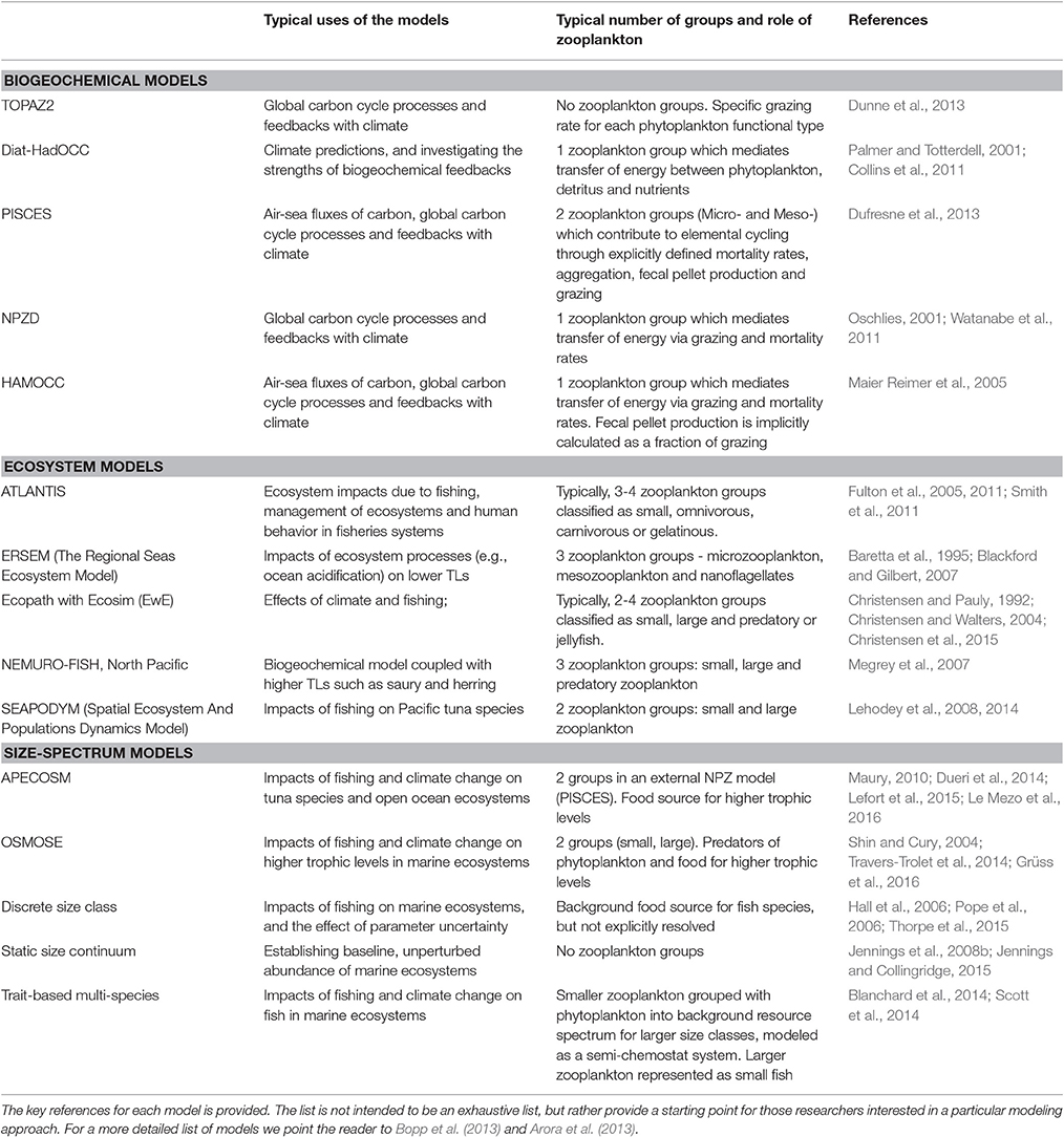
Table 1. A list of common biogeochemical, ecosystem and size-based models and how they represent zooplankton groups.
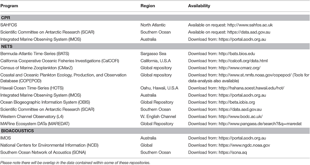
Table 2. A list of some zooplankton data repositories whose data can be used for model assessment.
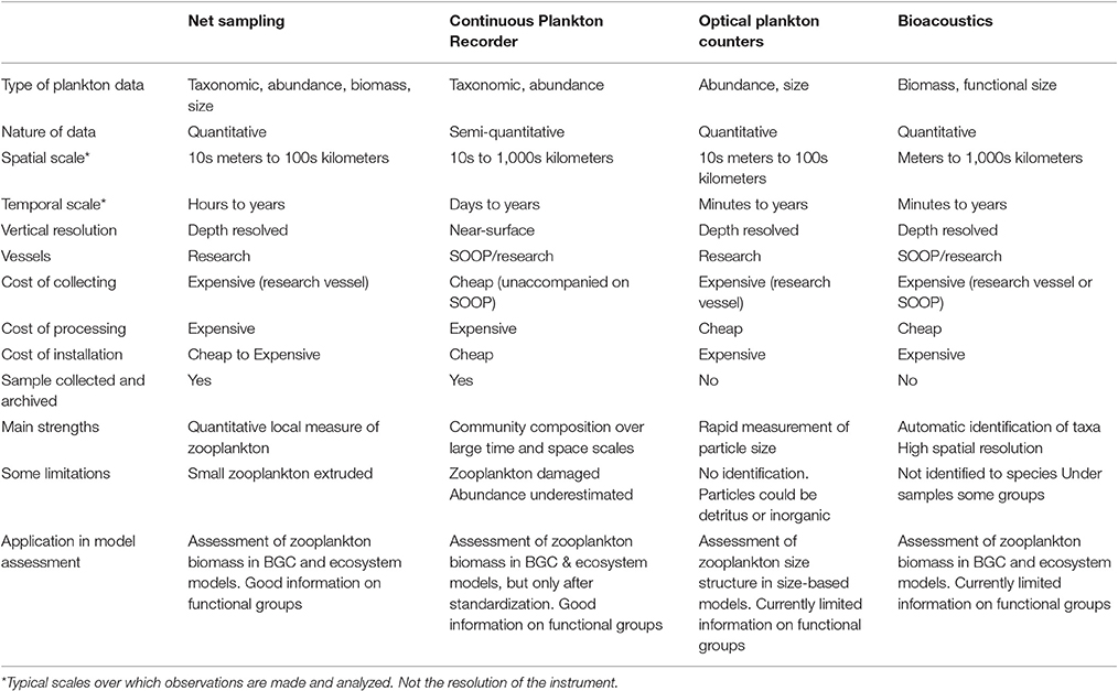
Table 3. An overview of the resolution, data type and strengths and weaknesses of the four main observation platforms described in this manuscript.
Our focus in this review is on assessment of zooplankton state variables (i.e., abundance and biomass pools) and we do not address better model parameterization (Mitra et al., 2014) or better representation of zooplankton functional groups (Le Quere et al., 2005) which have previously been well-reviewed. Additionally, we do not consider model initialization, although the approaches we suggest for model assessment are equally applicable. We also do not consider data assimilation, although we would highlight that the more modern observation approaches (e.g., laser optical plankton counters and bioacoustics) have considerable potential in this regard. This review will be useful for both zooplankton observationalists who want to produce useful data products for modelers, and modelers interested in new and robust ways of assessment of zooplankton biomass and abundance in their models.
Current Zooplankton Representation in Models
Biogeochemical Models
The classic structure of a marine biogeochemical model includes Nutrients, Phytoplankton, Zooplankton, Detritus (NPZD; Figure 1A). In the simplest NPZD structure, a single zooplankton compartment represents a broad spectrum of zooplankton and denotes the highest trophic level, which grazes on the single phytoplankton class (Wroblewski et al., 1988; Oke et al., 2013; Robson, 2014). In many biogeochemical models, if zooplankton are included, it is often as the top closure term (Steele and Henderson, 1992; Edwards and Yool, 2000), meaning that the mortality rate in the zooplankton compartment is treated as both a natural and predatory mortality rate. This releases nutrients held within the zooplankton back into the environment over time. Given this simple structure, it is arguable whether “zooplankton” included in some biogeochemical (lower trophic level) models can be considered to equate even conceptually with zooplankton in real systems. The “zooplankton” pool in these models must account for storage of all carbon and nutrients that has been taken up from phytoplankton and detritus by grazing but not yet returned to the pool of detritus and available nutrients through respiration and mortality, i.e., the biomass of all animals in the system.
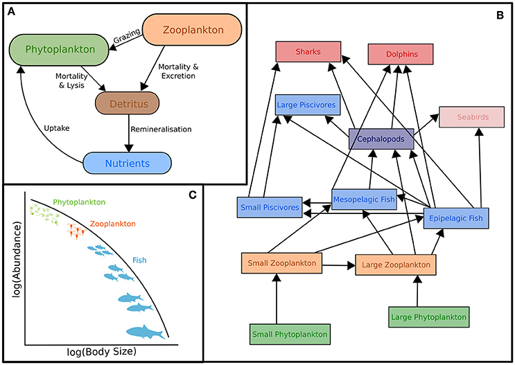
Figure 1. Representation of typical models featuring zooplankton: (A) Biogeochemical (NPZD or LTL) models, (B) Ecosystem models (HTL) and (C) Size-spectra models. Although not shown, all these models have temporal and spatial components. Individual-Based Models are not included in this schematic because they have many different forms which cover (A–C). For more information on IBMs see Section Individual Based Models and references therein.
In addition, many of the global biogeochemical models do not include a zooplankton compartment. Instead, the role of zooplankton is represented as an all-encompassing mortality rate for phytoplankton (Christian et al., 2010; Dunne et al., 2013; Holzer and Primeau, 2013; Matear and Lenton, 2014). Instead of explicitly modeling the interaction between primary and secondary consumers, these models include a parameter that captures the consumption of phytoplankton. These kinds of scaling parameters are rarely determined experimentally but rather they are tuned during model development and assessment to produce realistic model outputs for the region and parameter set (e.g., Holzer and Primeau, 2013).
Biological complexity can be increased within this simple NPZD structure to represent the lower trophic levels of marine ecosystems with various elemental cycles or to include multi-zooplankton compartments separated into different functional and/or size groups (Fennel and Neumann, 2004). The use of multiple phytoplankton functional groups based on physiology (Follows et al., 2007), taxonomy (Chan et al., 2002), or morphology (Kruk et al., 2010) is common, but the use of zooplankton functional groups is relatively less common. There are however some examples that distinguish zooplankton functional groups on the basis of grazing strategies and basal metabolism (Zhao et al., 2008) or feeding strategies, size and palatability to higher trophic levels (Sun et al., 2010). If we are to increase the complexity of zooplankton in a biogeochemical model, we not only need improved parameterization (Mitra, 2009), but also quantitative observations with which to help assess an expanded model that includes multiple zooplankton functional groups.
Ecosystem Models
Ecosystem models attempt to describe the whole ecological system, from primary producers to higher trophic levels, often including human components (Figure 1B). Generally, these models have complex predator-prey interactions, including dozens to hundreds of species. Zooplankton however, are generally only represented by a few classes (e.g., Yool et al., 2011; Piroddi et al., 2015; Table 2), defined by diet (Pinnegar et al., 2005), functional type (Le Quere et al., 2005), or size (Griffiths et al., 2010; Ward et al., 2012; Savina et al., 2013; Watson et al., 2013; Pedersen et al., 2016), or a combination of these. Of course, some ecosystem models have many more zooplankton classes (e.g., Pavés et al., 2013). Despite these exceptions, research using common ecosystem modeling approaches—ECOPATH with ECOSIM (Christensen and Walters, 2004), ATLANTIS (Fulton et al., 2005), ERSEM (Baretta et al., 1995), and SEAPODYM (Lehodey et al., 2008)—tend to focus on fish and fisheries (Griffiths et al., 2010) and are hindered by uncertainties in the prey and predator relationships of zooplankton (Mitra and Flynn, 2006). Of course, models (of any kind) do not need to represent every detail of the environment to be useful or address a specific question (Fulton et al., 2003), however we do know that zooplankton is essential to understanding the transfer of energy to fish and fisheries (Friedland et al., 2012; Lassalle et al., 2013), and therefore care needs to be taken in the representation of this link between the lower and upper tropic levels (Rose et al., 2010; Shin et al., 2010).
The simplification of zooplankton groups in ecosystem models, while not always ideal, enables operationalization of the model, however understanding the effects of climate variability and change on the target species or fisheries (for example), can only be understood if the trophic pathways leading to them are well-defined. A common problem with how zooplankton are represented in both ecosystem and biogeochemical models is the false assumption that the same zooplankton assemblage is present throughout the whole domain, both horizontally and vertically, and the structure of this assembly does not change over time (Ward et al., 2014). These models lump multiple zooplankton functional groups together and use an “average” set of parameter estimates. Zooplankton assemblages change markedly in character from eutrophic systems, dominated by the classic short food chains and larger species, to oligotrophic systems, dominated by longer food chains and smaller species. They differ vertically, with predatory and larger species below the euphotic zone and are further complicated due to the complexity of zooplankton behavior and life-cycle strategies such as molting and diapause. These changes, which fundamentally affect nutrient cycles and fisheries production, are often poorly represented in models.
Size-Based Models
The size-based approach to marine ecosystem modeling (Figure 1C) has developed as an alternative to more traditional taxonomy-based frameworks by simplifying the community structure through classifying individuals based on size as opposed to species identity (Figure 1C; Sheldon and Parsons, 1967; Sheldon et al., 1972; Andersen and Beyer, 2015; Andersen et al., 2016). Developed over the past 50 years, this approach is based on empirical observations that individual and community processes such as growth, respiration, and predator-prey relationships and trophic position all scale with body size (Peters, 1983; Jennings et al., 2001; Brown et al., 2004; Andersen et al., 2016). Size-based modeling has two main approaches: (1) static size spectra models (Trebilco et al., 2013) and (2) dynamic size spectra models (Blanchard et al., 2017). Similar to the trophic food web structuring of Lindeman (1942), discrete size spectrum models (or macroecological models) aggregate individual organisms into discrete trophic levels based on size (Jennings and Mackinson, 2003; Jennings et al., 2008a). In comparison, dynamic size spectrum models add the element of time, and scale individual size-based growth and mortality rates to the population and community level (Benoit and Rochet, 2004; Blanchard et al., 2009; Hartvig et al., 2011; Jacobsen et al., 2013; Maury and Poggiale, 2013; Dueri et al., 2014; Guiet et al., 2016).
How zooplankton are treated in size-based models depends on the primary focus. Most of these models focus on higher trophic levels and simply lump microzooplankton together with phytoplankton into a background food source for fish and macrozooplankton as “small fish”—i.e., using equations and parameters for metabolism and feeding for fish that are the size of zooplankton (Heneghan et al., 2016). This simplification eases computational costs, but has recently been called into question because lower trophic levels are critical to improving predictions of biomass and production at higher tropic levels in these models (Jennings and Collingridge, 2015).
Those models that have focused on zooplankton dynamics and food web structure explicitly resolve size-based zooplankton dynamics (Zhou and Huntley, 1997; Zhou, 2006; Baird and Suthers, 2007, 2010; Zhou et al., 2010), but do not explicitly include fish. To date, there have been few attempts to link these size-based zooplankton models to dynamic size spectrum models that have focused on higher trophic levels (but see OSMOSE; Shin and Cury, 2004). With increasing emphasis on understanding ecosystem impacts of climate variability and change, comes the need to better model bottom-up processes and thus the representation of zooplankton.
Individual Based Models
Individual based models (IBM) simulate individual animals, or groups of individuals as “superorganisms” that are treated as individuals. This allows a sophisticated representation of the behavior and/or physiology of each animal. For instance, IBMs can be structured so that they simulate the movements of animals in response to local light conditions (Batchelder et al., 2002), predator/prey encounters (Gerritsen and Strickler, 1977), or other environmental cues (Batchelder et al., 2002). In the planktonic environment, the main advantage of using an IBM is to account for rare individuals, circumstances or behaviors that contribute strongly to determining the overall population structure or variability; these are difficult to include in a state-variable approach (Werner et al., 2001). Rice et al. (1993), for example, show how variability in larval growth and survival rates can mean that the characteristics of a population of zooplankton can be quite different from the mean characteristics of the individuals within that population.
By simulating individual organisms, IBMs replicate the stochastic variability in the nutritional status, life-cycle stage, or behavior that exists within a population and that may have emergent implications for the overall properties of that population. These include modeling the variability in the survival of larval fish (Letcher et al., 1996), investigating implications of nutrition and reproductive status for food web dynamics of Daphnia (Perhar et al., 2016), the role of individual variability in physiological traits in sustaining zooplankton populations (Bi and Liu, 2017), and examining the effect of early/late diapause termination, food availability and initial stock size of the copepod Calanus finmarchicus in the Norwegian Sea (Hjøllo et al., 2012). This may come at a cost of increased model complexity and computational costs. In addition, IBMs require significantly more information on the modeled species if the model is to be rigorously parameterised and evaluated. As a result, IBMs are often applied to well-studied species such as the krill Euphausia pacifica (Dorman et al., 2015a,b) and the copepod C. finmarchicus (Skaret et al., 2014; Opdal and Vikebø, 2016). IBMs are also coupled to hydrodynamic, ecosystem or biogeochemical models (Skaret et al., 2014; Dorman et al., 2015a; Opdal and Vikebø, 2016; Parada et al., 2016), thus allowing two-way nesting within larger-scale modeling environments. Werner et al. (2001) reviewed the use of IBMs in marine modeling, while Breckling et al. (2006) provide a more general discussion of the use of IBMs in ecological theory.
Zooplankton Sampling Systems for Model Assessment
Before we discuss approaches to integrate zooplankton observations and models, we will briefly describe the major zooplankton sampling systems used for collecting zooplankton observations (Table 3), the different types of data each produces, and the characteristic temporal and spatial sampling scale, which includes the sampling extent, interval, and grain size (resolution).
There is no single best way to sample zooplankton. In the treatise by Wiebe and Benfield (2003), essential reading for observationalists and modelers, they describe 164 different zooplankton sampling systems, ranging from nets to optical sensors. This staggering variety of systems, each with distinct sampling characteristics, has evolved to answer specific zooplankton research questions, not for ease of uptake into models. Here we discuss four major types of zooplankton sampling systems that have been used in model assessment: nets; the CPR; size-based systems (e.g., OPC/LOPC and ZooScan); and bioacoustics (see Table 3).
Net Sampling
The use of nets is the oldest and most common method of sampling zooplankton. The recent history of zooplankton net sampling dates back to Thompson in 1828 (Wiebe and Benfield, 2003), but there are recorded observations prior to this (e.g., Sir Joseph Banks on the Endeavor in 1770; Baird et al., 2011). There are many different net configurations in use, but the key attributes that influence model assessment are the monitoring design, sampling characteristics, and the information derived from samples.
Sampling Characteristics
The large spatial and temporal extents of net sampling programs make their data well-suited for model assessment. Nets are used to collect zooplankton over a broad range of temporal extents—from hours to decades—and horizontal and vertical sampling grain sizes—from 10s of meters to 100s of kilometers (Table 3). The scale of a particular data set is usually dependent upon the aim of the survey. Process cruises tend to be one-off and are usually less useful for model assessment, unless the research cruise was specifically designed to answer a question that the model is addressing. Typically, data collected from long-term monitoring programs are more useful. Most monitoring programs involve point sampling, sampling weekly or monthly over many years. There are also many larger-scale surveys, often linked with fisheries assessments, that are collected seasonally or annually (e.g., CalCOFI: Edwards et al., 2010; or SARDI: Ward and Staunton-Smith, 2002).
There are four main characteristics to consider when using zooplankton data for model evaluation: type of tow, depth (and vertical resolution) of sampling, time of day, and mesh size. In terms of type of tow, nets can be dragged vertically, obliquely or more or less horizontally at specific depths (depth-stratified by an opening-closing net). All three types of net tows are good for sampling mesozooplankton (0.2–20 mm), although oblique and depth-stratified tows are better for capturing macrozooplankton (2–20 cm), as the net often has a larger mouth area and is towed faster, providing less opportunity for zooplankton to escape. Conversely, faster tow-speeds can result in increased extrusion of smaller individuals. Net avoidance of macrozooplankton such as Antarctic Krill can be minimized with the use of strobe-lights (Wiebe et al., 2004) which are thought to either “dazzle” the plankton, or attract them. Nets are typically towed in the mixed layer (top 50–100 m) or from near the seafloor to the surface. Nets that sample in the mixed layer during the day typically underestimate zooplankton abundance and biomass because larger zooplankton often vertically migrate out of the mixed layer during the day; thus, higher biomass is typically found during the night.
Mesh size is probably the most important net characteristic and varies depending on the size of the target group of zooplankton and the ecosystem of interest. Macrozooplankton are usually sampled with a larger mesh size—500 μm, for example, is commonly used for fish larvae. Historically, many researchers have used 330 μm mesh for mesozooplankton (Moriarty and O'Brien, 2013), but a finer mesh of 200 μm is now almost universally used in temperate and polar systems to better sample smaller zooplankton (Sameoto et al., 2000). However, fine mesh nets (100 μm) more quantitatively capture the smaller part of the mesozooplankton and some of the larger microzooplankton (e.g., juvenile stages of small copepods). Fine mesh nets are most commonly used in tropical areas where the zooplankton are generally smaller. Although coarse mesh nets extrude smaller zooplankton and thus underestimate abundance and biomass (Box 1), they still capture large organisms reasonably well (Sameoto et al., 2000).
Box 1. Data Wrangling: converting Zooplankton Biomass between Different Units.
Model assessment using zooplankton biomass is not as straightforward as it might seem because observationalists use a range of different measures, from volumetric to elemental measures, of zooplankton biomass. Table B1 briefly outlines the different units used to measure zooplankton biomass; for detailed information on the various methods see Postel et al. (2000). These different measures of zooplankton biomass all have their different strengths and weaknesses. We have ordered the rows of Table B1 by the robustness of the different methods and the ease in which they can be used in modeling, ranging from the most imprecise (Settled Volume) to the most robust (Carbon Mass).
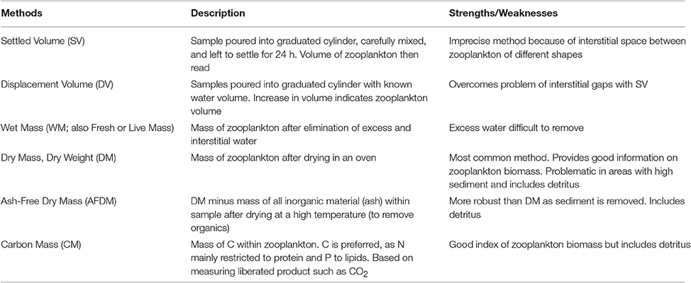
Table B1. Glossary of zooplankton biomass terms, and their strengths/weaknesses.
Most models usually use a currency of Nitrogen (or sometimes Carbon) biomass, which is rarely measured. Table B2 provides a series of equations to convert different biomass to Carbon Mass. Once estimates are in Carbon Mass, they can be converted to Nitrogen Mass by using the C:N ratio of zooplankton, which typically varies from 4:1 to 6:1, but is commonly 5:1 (Postel et al., 2000).
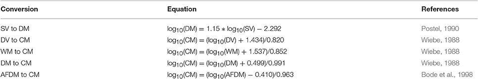
Table B2. Equations to convert different biomass methods to carbon mass, Rearranged from Postel et al. (2000).
Information Derived from Net Samples
For model assessment, probably the simplest and most useful information derived from net samples is zooplankton biomass. Biomass is measured in several different ways: settled volume, displacement volume, wet weight, dry weight, or occasionally carbon (Postel et al., 2000). Each is measured on different scales, and can be converted from one to another using standard conversions (Box 1). Occasionally, samples are poured through meshes of several different sizes and then weighed, providing biomass in different size categories (Huo et al., 2012; Banaru et al., 2014). Other information available from net samples is typically some idea of the zooplankton community present. This can vary from a coarse identification of the community (e.g., copepods, chaetognaths, jellyfish) to species-level identification. Taxonomic identification allows for use in IBM, or the subsequent aggregation of data into functional groups that might be represented in ecosystem models (e.g., mesozooplankton, herbivores, calcifiers).
The Continuous Plankton Recorder
The CPR has been used for the past 85 years to sample over large regions of the North Atlantic Ocean, and has spawned surveys in the North Pacific Ocean, Southern Ocean, around Australia, and in southern Africa. Unlike nets, there is only one main CPR design that has remained relatively unchanged over the years (Reid et al., 2003). Key attributes of the CPR that influence model assessment are monitoring design, its sampling characteristics, and the information derived from the samples (Richardson et al., 2006).
Sampling Characteristics
The large spatial and temporal extents characteristic of CPR surveys make the data well-suited for model assessment. The CPR collects zooplankton over greater time and space scales than net sampling—from days to decades and from 10s of kilometers to 1,000s of kilometers (Table 3). The temporal grain size (duration of a transect segment) is 15–30 min and the sampling interval between transects is typically a month or longer. The horizontal resolution (length of a transect segment) is 10–20 km. The CPR is not used for short-term process studies, but is deployed routinely by commercial vessels plying common shipping routes, making it ideal for studying trends over time (Richardson et al., 2006).
The CPR is towed near-surface (~7 m), but the draft of the large towing vessels probably mixes water down to 15 m. The aperture of the CPR is small (1.27 × 1.27 cm) and prevents large macrozooplankton such as jellyfish (scyphomedusae) from entering, although small and juvenile euphausiids are sampled (Hunt and Hosie, 2003). Fragile organisms, such as gelatinous plankton, are poorly sampled by the CPR because they are damaged when they come in contact with the silk mesh. For more detailed information about CPR sampling characteristics, see Richardson et al. (2006).
It is well-known that the CPR provides semi-quantitative rather than truly quantitative estimates of zooplankton abundance (Clark et al., 2001; John et al., 2001; Batten et al., 2003; Richardson et al., 2004, 2006), underestimating absolute numbers of zooplankton, but relative changes through time and over space are robust (see Section Simple Observation Models: Simulated Sampling from a Model). Small zooplankton are likely to be under-sampled because of extrusion through the relatively large mesh size of silk used in the CPR (270 μm) compared with standard nets (Sameoto et al., 2000). Large zooplankton are likely to be under-sampled by the CPR because of active avoidance (Clark et al., 2001; Hunt and Hosie, 2003; Richardson et al., 2004).
Notwithstanding the semi-quantitative nature of CPR sampling, it captures a roughly consistent fraction of the in situ abundance of each taxon and thus reflects the major patterns observed in the plankton (Batten et al., 2003). Seasonal cycles estimated from CPR data for relatively abundant taxa are repeatable each year (Edwards and Richardson, 2004) and show good agreement with other samplers such as WP-2 nets (Clark et al., 2001; John et al., 2001) and the Longhurst Hardy Plankton Recorder (Richardson et al., 2004). Inter-annual changes in plankton abundance are also captured relatively well by the CPR (Clark et al., 2001; John et al., 2001; Melle et al., 2014) because the time-series has remained internally consistent, with few changes in the design of the CPR or in counting procedures.
Information Derived from CPR Samples
Data from the CPR are zooplankton abundance, with no direct estimate of biomass. Data are normally expressed in numbers per sample. Although each sample represents ~3 m3 of filtered seawater, abundance estimates are seldom converted to per m3 estimates in practice because of their semi-quantitative nature.
As with net samples, a strength of CPR data is that taxonomic information is available. Typically, the copepods are well-resolved to species and the other groups to higher taxonomic levels (see Table 5 in (Richardson et al., 2006) for the taxa counted). This means that the data may be aggregated into functional groups that equate to those in models (e.g., Lewis et al., 2006). The CPR also retains phytoplankton (although not quantitatively) because of the leno silk weave of the mesh (see Richardson et al., 2006 for details). Phytoplankton are counted to the lowest possible level using light microscopy and these data can be aggregated into phytoplankton functional groups that equate to those in models, such as diatoms and dinoflagellates, and used for model assessment alongside zooplankton data (e.g., Lewis et al., 2006).
Optical Plankton Counters
The most common instruments for measuring in-situ size spectra are the Optical Plankton Counter (Herman, 1988) and Laser Optical Plankton Counter (Herman, 2004). These instruments use either light emitting diodes-LEDs (LED-OPC) or lasers (LOPC) to measure the optical density and cross-sectional area of each particle as it passes through the sampling tunnel, and thereby estimate surface area (Sprules and Munawar, 1986; Suthers et al., 2006; Basedow et al., 2010). Hereafter we generalize, and refer collectively to both instruments as an OPC.
Sampling Characteristics
The large temporal and/or spatial extents and high temporal and spatial resolutions characteristic of OPC deployments make the data well-suited for model assessment. The OPC collects information of the size-spectra of zooplankton over a broad range of temporal and spatial extents—from minutes to years and from 10s of meters to 100s of kilometers (Table 3). Due to the continuous electronic data collection of OPCs, there is no typical grain size (length of sample segment), and it depends largely on the purpose of the study and deployment method. OPCs can be deployed vertically (Vandromme et al., 2014; Marcolin et al., 2015; Wallis et al., 2016), mounted on a towed undulating vehicle to obtain high-resolution estimates of size spectra through space and time (Zhou et al., 2009; Everett et al., 2011; Basedow et al., 2014), mounted on a net frame (Herman and Harvey, 2006; Checkley et al., 2008; Marcolin et al., 2013), integrated with autonomous floats (Checkley et al., 2008), or mounted in the laboratory for the processing of net-samples (Moore and Suthers, 2006). OPCs are capable of sampling through the water column (up to 660 m deep) and if mounted on a towed body, over regional scales (100s km). OPCs are only deployable on research vessels for a range of reasons including: they need a trained technician to monitor them, require power via the tow-cable (or regular changing of data-logger batteries) and cannot be towed at the full speed of most commercial vessels. Therefore, unlike the CPR, they are not suited to ships of opportunity.
Taxonomic information is not directly available from OPCs, but they are often partnered with net samples, either by mounting within the net mouth (Herman, 2004) or as part of a broader sampling program whereby net and OPC samples are taken in close proximity to provide species-specific information, particularly for mono-cultures (e.g., overwintering C. finmarchicus; Gaardsted et al., 2011 or swarms of Thalia democratica; Everett et al., 2011). As for all sampling techniques, gear avoidance and sampling volume can be a problem when zooplankton abundance is low (Basedow et al., 2013), due to the small aperture of the OPC (20–49 cm2) however these can be partially resolved by towing at a higher speed or for longer periods. Size-based data are also available from other instruments such as the in-situ Video Plankton Recorder (Davis et al., 2004) or the lab-based ZooScan (Vandromme et al., 2014 requires net samples). Inter-comparisons of size spectra between LOPC and ZooScan (Schultes and Lopes, 2009; Vandromme et al., 2014; Marcolin et al., 2015) or LOPC and VPR (Basedow et al., 2013) have shown mixed results. The biggest differences between ZooScan and the LOPC are thought to be due to the sampling of sediment in the small size-classes by the LOPC in coastal areas (Schultes and Lopes, 2009), although techniques have been developed to account for this (Jackson and Checkley, 2011) and can result in improved correlations between LOPC and ZooScan (Marcolin et al., 2015).
Information Derived from OPC
The key strength of OPCs is their ability to quantify abundance, size and biovolume of plankton simultaneously over a large size range (0.1–35 mm for LOPC; Herman, 2004). In particular, OPCs are ideal for comparison with size-based models as they share the common currency of size and abundance. One common way to represent the size-distribution of plankton in the ocean is the normalized biomass size spectrum (NBSS; Silvert and Platt, 1978). The NBSS is a histogram-style size-distribution, in which the biovolume (or biomass) in a size class is normalized by the width of the size-class, such that the normalized distribution is independent of the width of size-classes (Platt and Denman, 1977). Using size-spectra theory, it is possible to extract trophic level and growth and mortality rates from in-situ OPC data (Edvardsen et al., 2002; Zhou, 2006; Basedow et al., 2014).
Other Optical Instruments
While OPCs are the most common in-situ optical instruments, the field is developing rapidly and there are a range of other systems which deserve to be mentioned. In particular, camera and imaging systems such as ZooScan (Laboratory only; Grosjean et al., 2004), FlowCam (Laboratory only; Sieracki et al., 1998), Zooplankton Visualization system (ZOOVIS; Trevorrow et al., 2005), Video Plankton Recorder (VPR; Davis et al., 2005), Lightframe On-sight Keyspecies Investigation (LOKI; Schmid et al., 2016), and the In Situ Ichthyoplankton Imaging System (ISIIS; Cowen and Guigand, 2008) have become more widespread. Additionally, increased effort has been invested in the identification of zooplankton from images (Zooniverse, www.planktonportal.org). The highly depth-resolved individual images from these systems provide detailed information on both taxonomy and individual features (e.g., proportion of females carrying egg sacs) which will be beneficial to model assessment of IBM's. Moreover, developing artificial intelligence techniques (Layered neural networks, random forest algorithm and evolutionary algorithms) have permitted impressive advances in the automated detection of such features (Bi et al., 2015) and will add significant value to these optical systems.
Bioacoustics
Sampling Characteristics
Bioacoustic data can provide estimates of zooplankton and fish distribution, behavior and abundance using soundwaves and knowledge of the target strength of individual taxa (Foote and Stanton, 2000; Simmonds and MacLennan, 2005). Bioacoustic systems operate over fine to large scales, and are able to measure horizontal and vertical scales simultaneously (Table 3). Bioacoustic data for zooplankton can be obtained from single, multiple and broad band frequencies using ship-based systems or fixed platforms such as moorings (Godø et al., 2014). For mesozooplankton (~0.2–20 mm) high frequencies are used from 100 KHz to 10 MHz in moored or profiling devices to resolve the size classes and types of organisms (Holliday et al., 2009). Acoustical backscatter from zooplankton are collected by the acoustic receiver and analyzed to estimate biomass or relative change in biomass of dominant scattering groups (Holliday and Pieper, 1995; Lavery et al., 2007; Kloser et al., 2009; Godø et al., 2014; Irigoien et al., 2014; Lehodey et al., 2014). The spatial resolution can be increased by moving the acoustic sensor, by using multiple spatially distributed sensors, or by tracking organisms within the acoustic beam (Godø et al., 2014). The temporal resolution of the backscatter can be improved by increasing the ping rates to resolve an individual's distribution and behavior patterns (Holliday et al., 2009; Godø et al., 2014).
Bioacoustic techniques offer a number of advantages over traditional net or CPR sampling because they provide high-resolution data at both spatial (horizontal and vertical) and temporal scales depending on the deployment platform. High-frequency, broadband systems enhance the sampling resolution to millimeter scale so that smaller targets, such as copepods, can be quantified (Holliday et al., 2009; Godø et al., 2014). Where patches of plankton and fish are small (Benoit-Bird et al., 2013), plankton nets and the CPR do not provide an accurate picture of the spatial distribution of the organisms that they capture as the sampling volumes are far larger than the patches (Godø et al., 2014). In addition, bioacoustics can provide better biomass estimates when combined with other methods such as nets (Kaartvedt et al., 2012) as there are minimal gear avoidance problems.
Information Derived from Bioacoustics
Raw data from bioacoustics platforms is backscatter intensity over a single multiple or broad band of frequencies. A skilled analyst, using in isolation or a combination of scattering models, nets or optical sampling, is able to convert backscatter intensity to estimates of either biomass, abundance or (with more difficulty) broad taxa or potentially size groups (Holliday et al., 2009) depending on the region being considered. The high spatial and temporal resolution of these data are ideal for integration with modeling techniques. In the case of zooplankton, a major complicating factor in the use of multi-frequency bio-acoustic techniques is the diversity of this community, where a wide range of organisms of different sizes, shapes, orientations, and material properties occur together in the water column (Holliday and Pieper, 1995; Lavery et al., 2007). All these characteristics, along with their behavior, influence the way in which they scatter sound. To estimate their individual acoustic reflectance or target strength (TS), a series of zooplankton sound scattering models have been developed (Table 1 from Lavery et al., 2007) to account for that diversity.
Zooplankton Data in Model Assessment
The performance of the zooplankton component of numerical models is rarely assessed against field observations because, unlike other parameters such as temperature or chlorophyll a biomass, observations of zooplankton do not generally resemble the resolution of the modeled zooplankton variables (temporally or spatially), are in a very different format (species abundance rather than mass of nitrogen), or are inaccessible (e.g., hidden in gray literature/personal collections). Because zooplankton observations are collected using a range of platforms that measure different parameters such as abundance (e.g., CPR, nets, bioacoustics), size (e.g., LOPC) or biomass (e.g., nets), model assessment requires uncertain and generally species- and location-dependent conversion factors (Arhonditsis and Brett, 2004) to approximate the zooplankton biomass in models (Postel et al., 2000). This makes it difficult to compare modeled zooplankton information with observed data. To address this challenge, we turn our focus to a discussion of the two primary ways to link zooplankton in models with zooplankton observations: (1) data wrangling that transforms observational data to be directly comparable with model outputs; and (2) observation models that transform model output to be more comparable with observational data.
Data Wrangling: Transforming Observational Data to Be More Like Model Outputs
Data wrangling is the process of iterative data exploration and transformation from one format to another to make them more useful (Kandel et al., 2011). We use the term here to describe the series of steps that transforms observational data into a form that is more comparable with model output. Data wrangling transforms observed data into model-ready datasets. Data wrangling takes many forms, but two of the most important are conversion of observed biomass into appropriate values to compare with model estimates (see Box 1 for details), and collating biomass estimates collected using nets with different mesh sizes or different sampling devices (see Box 2 for details).
Box 2. Data Wrangling: Converting Zooplankton Biomass between Different Mesh Sizes and Using Proxy Estimates
Different mesh sizes: Different mesh sizes of nets provide very different biomass values, with higher zooplankton biomass estimates from finer mesh nets. To convert biomass data collected with different mesh sizes to an equivalent mesh size, common conversions can be applied (Table B3; Moriarty and O'Brien, 2013), although it must be acknowledged that the best conversion is dependent upon the zooplankton assemblage present. Fortunately, different net systems produce similar estimates of zooplankton when operated with similar mesh sizes (Skjoldal et al., 2013).
Table B3. Equivalent mesh size conversions (modified from Moriarty and O'Brien, 2013).
Proxy estimates—Abundance: Sometimes zooplankton abundance and not biomass is measured. It is difficult to convert abundance to biomass because you do not know the size of individuals and thus their mass. In this situation, we recommend using abundance data for relative patterns—for example seasonal cycles, spatial variation, or inter-annual variation. Lewis et al. (2006) assessed their ecosystem model by normalizing both the model biomass and the observed abundance data and comparing the normalized patterns spatially and temporally.
Proxy estimates—Biovolume: Size-based methods of measuring zooplankton (LOPC/OPC/VPR/ZooScan) can provide estimates of zooplankton biomass. These instruments measure organism size (2-D area) and this can be converted to organism volume. Biovolume can then be converted to biomass by summing organism volume across all individuals and assuming zooplankton has the same density of seawater. Zooplankton biomass from the VPR and ZooScan has the advantage that detritus and sediment can be removed. An advantage of these size-based methods are that they can be used to estimate biomass in size classes. They could also be used to partition observed zooplankton total biomass into size classes (i.e., using the size spectra to estimate the % of biomass in different size classes and applying this to measured biomass).
One example of data wrangling is finding the optimal way to interpolate scattered observations onto a regular model grid at a fixed point in time (Buitenhuis et al., 2013; Moriarty and O'Brien, 2013). A more complex example is the conversion of observed zooplankton abundance (or biovolume) to nitrogen (or carbon) biomass, which is how many models represent zooplankton biomass (Box 1). This approach requires assumptions about the size distribution and stoichiometry of zooplankton in the sample. Given these assumptions, modelers are able to use these data, but need to understand the basis of the assumptions that are made, and the magnitude of the error inherent in the conversion.
Often gridded data products—think of the global chlorophyll a products—are the most readily used for model assessment of phytoplankton. Similarly, the wrangling of 153,163 zooplankton biomass values, from a variety of locations, formats and collection methods, into a freely-available gridded global database of consistent biomass units was an amazing effort (COPEPOD; http://www.st.nmfs.noaa.gov/copepod/; Moriarty and O'Brien, 2013). Unlike chlorophyll a however whose global satellite maps are updated daily, the time-consuming nature of zooplankton collection means there isn't a truly global database (see gaps in Figure 2) which is updated on time-scales relevant to many modeling studies. These data are extremely useful however, to constrain model estimates by providing biomass limits against which to assess our models. There are many statistical tools available to assist with the practical side of data-wrangling (e.g., “tidyr” or “dplyr” in R), but the most important aspect is dialogue between modelers and observationalists.
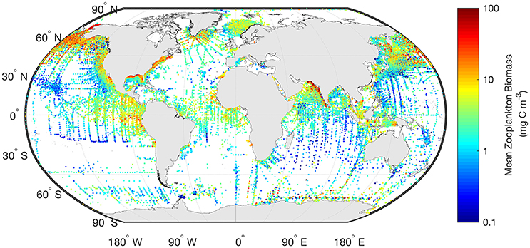
Figure 2. The mean marine zooplankton biomass (mg C m−3) for mesozooplankton (0–200 m depth) is shown illustrating the distribution of records from the most comprehensive database available. The data shown here are freely available from “COPEPOD: The Global Plankton Database” (http://www.st.nmfs.noaa.gov/copepod/).
Observation Models: Transforming Model Output So It Is More Like Observational Data
Where zooplankton observations are incorporated into models, there is often a mismatch between the observations (often infrequent point measurements) and the high spatial and temporal resolution of models. Observation models are one technique that can help address these mismatches, allowing model assessment at a range of scales. We define an observation model as a model that takes the output of a simulation and transforms it to a form that closely resembles the observations with which it is being compared. This approach of generating observations from models is used in numerical weather prediction (Dee et al., 2011), acoustic observations of mid-trophic levels (Handegard et al., 2012), and remotely-sensed ocean color observations (Baird et al., 2016).
The observation model needs to be based on sufficient process understanding, so that it applies well over a broad range of environments and the error in the output of the observation model is due primarily to the simulation model estimate (i.e., zooplankton biomass) and not the accuracy of the parameters or equations within the observation model itself. Essentially, the rationale of an observation model is to allow comparison of observed and modeled data, by removing inconsistencies in the structure or scale of these data. Here we review some of the steps and challenges to developing zooplankton observation models, for improved interpretation of the observations and assessment of numerical models. Below we discuss the range of observation models, from simple to more complex.
Simple Observation Models: Simulated Sampling from a Model
The simplest approach to developing an observation model is to undertake simulated sampling within a model, and compare these sampled data to zooplankton observations. For example, zooplankton biomass estimates can be extracted from a simulation corresponding to the time, location, and depth of the samples collected by nets, CPR, OPC, or bioacoustics. While not directly comparing their model to observations, Wiebe and Holland (1968) were likely the first to simulate net tows within a computer simulation when they determined the effect of net size and patchiness on sampling error.
An example using the CPR highlights the approach of simulated sampling from a model. Lewis et al. (2006) compared the abundance of zooplankton as measured by the CPR with plankton output from an ecosystem model of the Northeast Atlantic Ocean. Simulated “tows” were performed by extracting biomass data of omnivorous mesozooplankton from the model at the time (day and nearest hour), location (longitude and latitude), and depth (7 m) of corresponding samples collected by the CPR (Figure 3). Because the CPR provides semi-quantitative abundance estimates, and not biomass (Richardson et al., 2006), both the samples and corresponding model output were standardized to a mean of zero and a unit standard deviation to produce a dimensionless z-score (Cheadle et al., 2003). This allowed a direct semi-quantitative evaluation of spatio-temporal model performance of omnivorous mesozooplankton. This evaluation highlighted that the model had the ability to reproduce the main seasonal features such as the spring and autumn blooms, and plankton succession observed in the CPR data and showed good correlation between magnitudes of these features with respect to standard deviations from a long-term mean. The model assessment also highlighted differences in the timing of patterns in phytoplankton seasonality (e.g., spring diatom bloom in the model is too early), allowing the reparametrizing of the model (Lewis et al., 2006).
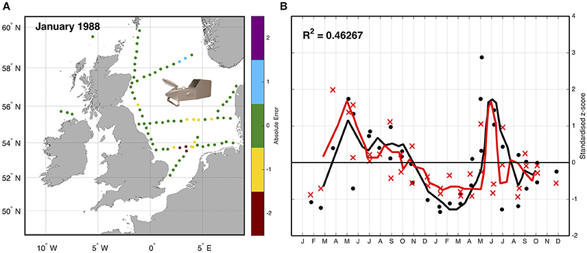
Figure 3. Sampling the model—(A) Simulated “tows” within the model were performed by extracting biomass data of omnivorous mesozooplankton from the exact time (day and nearest hour), location (longitude and latitude), and depth (7 m) of corresponding samples collected by the CPR. (B) The data are then standardized due to the different units, and the difference between normalized z -scores for both simulation and observation between January 1988 and December 1989 with a 3-day running mean (solid line) is shown. Black is model data, red is CPR data; dots are individual model tow points, crosses are individual CPR tow points (redrawn from Lewis et al., 2006).
More Complex Observation Models: Add-On Models That Convert Output to Observations
With improving technologies and computing power comes the opportunity to embrace increasingly complex observation models. Here we borrow many examples from state-of-the-art applications in other fields of model assessment that have not yet been fully applied to zooplankton. These are ideally suited for the assessment of zooplankton models due to the inherent disconnect between the spatial and temporal resolution and model currency of observations and models.
Historically, in phytoplankton model assessment, satellite-derived chlorophyll a is compared with modeled phytoplankton (Oschlies and Schartau, 2005; Lacroix et al., 2007; Gregg, 2008; Brewin et al., 2010; Kidston et al., 2011, 2013), but inaccuracies in both the satellite observation (e.g., measurement error due to CDOM in the water) and conversion of model units (e.g., conversion of nitrogen biomass to chlorophyll a) introduce errors into the model assessment. To limit these inaccuracies, Baird et al. (2016) used an optical observation model, nested within a biogeochemical model, to assess water-leaving irradiance from the model, against satellite-derived water-leaving irradiance. The water-leaving irradiances, from the observation model and the satellite, can be directly compared against each other to assess the model. Alternatively, the water-leaving irradiance measures from both the observation model and the satellite, can be converted to chlorophyll a using one of the satellite algorithms in order to allow a comparison which may be more informative for those used to thinking about chlorophyll a. In either case, both the units of assessment, and the method used to derive them, are the same. Thus, the mismatch between simulated and observed remote-sensing reflectance provides an excellent metric for model assessment of the coupled biogeochemical model (Baird et al., 2016; Jones et al., 2016).
This approach—of building an observation model that enables the model to produce information more comparable to observations—has not yet been applied to zooplankton but would be a valuable way forward. For zooplankton model assessment, building observation models for size-spectra models would be fairly straightforward given that observational techniques (OPC, ZooScan and VPR) measure the size and abundance of the zooplankton community—metrics easily extracted from size-spectra models. It is also made easier because size spectra are typically represented as Normalized Biomass Size Spectra (NBSS; Section Optical Plankton Counters), where size classes are normalized by the width of the size-class, making the shape of the spectrum independent of the size-classes chosen (Platt and Denman, 1977). The NBSS can thus be generated from both the observations and models, even if they each have different size-resolutions. In addition to comparing state-variables, the size-based approach developed by Zhou (2006), Zhou et al. (2010) provides an intuitive framework for estimating time-averaged rates (e.g., growth, mortality) for zooplankton from observed NBSS, which could then be tested within dynamic size spectrum models that include zooplankton (Heneghan et al., 2016) or compared to observed rates in the field (Zhou et al., 2010).
Another potential area for development of an observation model is in bioacoustics. Traditional outputs from zooplankton bioacoustic observations are the distribution, behavior, biomass and abundance of trophic levels, size categories, or species of interest derived from scattering models (Lavery et al., 2007; Holliday et al., 2009; Kloser et al., 2009; Godø et al., 2014). These scattering model measures can then be used to assess ecosystem models (Luo and Brandt, 1993; Holliday et al., 2009; Kloser et al., 2009). This requires the aggregation of focal taxa from the ecosystem model output and conversion to a common currency. This need to transform both observation and model outputs to a common format introduces error and inconsistencies into each. An alternative approach is to create a bioacoustic observation model which uses scattering models to estimate the backscatter intensity of zooplankton within the ecosystem model and compare this to bioacoustic observations in the ocean (Figure 4; Handegard et al., 2012). The main challenge for the observation model is to simulate the observed backscatter at a particular frequency and depth within the model. In this case, we are not directly modeling sound within the ecosystem model, so this observation model does not provide feedback (external forcings or changes in state variables) to the ecosystem model. It is simply about avoiding inconsistencies in the comparison of modeled and observed data, and enabling the comparison of “like with like.” Building such an acoustic observation model would simulate acoustic observations, producing an echogram (Figure 4). Thus, for all model points in time and space, the observation model could produce an echogram based on the zooplankton functional groups predicted by the ecosystem model. As with all model-observation comparisons, care must be taken to consider the temporal and spatial resolution measured or modeled. In the case of bioacoustics, the measurements will often be at a higher spatial resolution (meters; Table 3), but lower temporal resolution (minutes; Table 3) than the model. High-resolution bioacoustic measurements of abundance and biomass can be downscaled to match the resolution of ecosystem models. Clean acoustic observations will need to be readily available for comparison with the simulated outputs of the observation model, which could be achieved with the use of a multi-frequency acoustic mooring, which delivers acoustic data resolved vertically and temporally at a single site (Urmy et al., 2012).
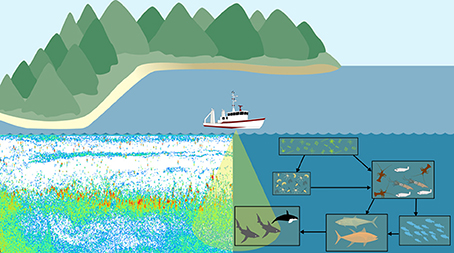
Figure 4. A bioacoustic observation model would apply the same scattering models to both the backscatter measurements from the ocean and the ecosystem model. Regardless of environment (ocean or model), we can use the same principle of the scattering models to produce echograms which can be directly compared.
Concluding Remarks
In this review, we summarize many of the fundamentals of zooplankton modeling for observationalists and zooplankton observations for modelers. As highlighted by Flynn (2005), we believe that there needs to be greater discussion and collaboration between modelers and observationalists. Only through dialogue will we be able to perform the data wrangling and develop the observation models that are needed so our observations and model outputs align. In particular, observation models have not been applied in the assessment of zooplankton in models and are likely to be a powerful approach, as they have been in other disciplines. These observation models range from the simple (sampling the model) to the more complex (bioacoustics) and can even result in the underlying model being changed to output data that is directly comparable to the observations (e.g., water leaving irradiance and chlorophyll a). The development and use of complex observing models can be time consuming, but many of the techniques described above are already being implemented (Handegard et al., 2012; Baird et al., 2016). The adoption of these ideas for use in zooplankton research would be a major step forward, allowing zooplankton observations to be more readily used in model assessment as real-time data becomes a possibility with optical and acoustic systems. Here we have provided a few ideas. We hope that this review will increase the dialogue between modelers and observationalists, and provide the impetus for greater model assessment of zooplankton output through data wrangling and state-of-the-art observation models.
Author Contributions
JE, AR, and MB conceived the original idea for this workshop and manuscript. All authors contributed to the writing of the manuscript. JE and AR wrote the final draft.
Conflict of Interest Statement
The authors declare that the research was conducted in the absence of any commercial or financial relationships that could be construed as a potential conflict of interest.
Acknowledgments
This manuscript was written as part of the Integrated Marine Observing System (IMOS) “Zooplankton Ocean Observing and Modelling” workshop held in Hobart 15–16 February 2016. The workshop was funded by IMOS. JE was funded by an Australian Research Council Discovery Grant (DP150102656). The CPR and fauna images in Figures 1, 4, and 5 were provided by the Integration and Application Network, University of Maryland Center for Environmental Science (ian.umces.edu/imagelibrary/).
References
Andersen, K. H., and Beyer, J. E. (2015). Size structure, not metabolic scaling rules, determines fisheries reference points. Fish Fish. 16, 1–22. doi: 10.1111/faf.12042
Andersen, K. H., Berge, T., Gonçalves, R. J., Hartvig, M., Heuschele, J., Hylander, S., et al. (2016). Characteristic sizes of life in the oceans, from bacteria to whales. Annu. Rev. Mar. Sci. 8, 217–241. doi: 10.1146/annurev-marine-122414-034144
Arhonditsis, G. B., and Brett, M. T. (2004). Evaluation of the current state of mechanistic aquatic biogeochemical modeling. Mar. Ecol. Prog. Ser. 271, 13–26. doi: 10.3354/meps271013
Ariza, A., Garijo, J. C., Landeira, J. M., Bordes, F., and Hernandez-Leon, S. (2015). Migrant biomass and respiratory carbon flux by zooplankton and micronekton in the subtropical northeast Atlantic Ocean (Canary Islands). Prog. Oceanogr. 134, 330–342. doi: 10.1016/j.pocean.2015.03.003
Arora, V. K., Boer, G. J., Friedlingstein, P., Eby, M., Jones, C. D., Christian, J. R., et al. (2013). Carbon–concentration and carbon–climate feedbacks in CMIP5 earth system models. J. Clim. 26, 5289–5314. doi: 10.1175/JCLI-D-12-00494.1
Baird, M. E., and Suthers, I. M. (2007). A size-resolved pelagic ecosystem model. Ecol. Modell. 203, 185–203. doi: 10.1016/j.ecolmodel.2006.11.025
Baird, M. E., and Suthers, I. M. (2010). Increasing model structural complexity inhibits the growth of initial condition errors. Ecol. Complexity 7, 478–486. doi: 10.1016/j.ecocom.2009.12.001
Baird, M. E., Cherukuru, N., Jones, E., Margvelashvili, N., Mongin, M., Oubelkheir, K., et al. (2016). Remote-sensing reflectance and true colour produced by a coupled hydrodynamic, optical, sediment, biogeochemical model of the Great Barrier Reef, Australia: comparison with satellite data. Environ. Modell. Softw. 78, 79–96. doi: 10.1016/j.envsoft.2015.11.025
Baird, M. E., Everett, J. D., and Suthers, I. M. (2011). Analysis of southeast Australian zooplankton observations of 1938–42 using synoptic oceanographic conditions. Deep Sea Res. Part II Top. Stud. Oceanogr. 58, 699–711. doi: 10.1016/j.dsr2.2010.06.002
Banaru, D., Carlotti, F., Barani, A., Gregori, G., Neffati, N., and Harmelin-Vivien, M. (2014). Seasonal variation of stable isotope ratios of size-fractionated zooplankton in the Bay of Marseille (NW Mediterranean Sea). J. Plankton Res. 36, 145–156. doi: 10.1093/plankt/fbt083
Baretta, J. W., Ebenhoh, W., and Ruardij, P. (1995). The european-regional-seas-ecosystem-model, a complex marine ecosystem model. Neth. J. Sea Res. 33, 233–246. doi: 10.1016/0077-7579(95)90047-0
Basedow, S. L., Tande, K. S., and Zhou, M. (2010). Biovolume spectrum theories applied: spatial patterns of trophic levels within a mesozooplankton community at the polar front. J. Plankton Res. 32, 1105–1119. doi: 10.1093/plankt/fbp110
Basedow, S. L., Tande, K. S., Norrbin, M. F., and Kristiansen, S. A. (2013). Capturing quantitative zooplankton information in the sea: performance test of laser optical plankton counter and video plankton recorder in a Calanus finmarchicus dominated summer situation. Prog. Oceanogr. 108, 72–80. doi: 10.1016/j.pocean.2012.10.005
Basedow, S. L., Zhou, M., and Tande, K. S. (2014). Secondary production at the polar front, barents sea, August 2007. J. Mar. Syst. 130, 147–159. doi: 10.1016/j.jmarsys.2013.07.015
Batchelder, H. P., Edwards, C. A., and Powell, T. M. (2002). Individual-based models of copepod populations in coastal upwelling regions: implications of physiologically and environmentally influenced diel vertical migration on demographic success and nearshore retention. Prog. Oceanogr. 53, 307–333. doi: 10.1016/S0079-6611(02)00035-6
Batten, S. D., Clark, R., Flinkman, J., Hays, G., John, E., John, A. W. G., et al. (2003). CPR sampling: the technical background, materials and methods, consistency and comparability. Prog. Oceanogr. 58, 193–215. doi: 10.1016/j.pocean.2003.08.004
Benoit, E., and Rochet, M. J. (2004). A continuous model of biomass size spectra governed by predation and the effects of fishing on them. J. Theor. Biol. 226, 9–21. doi: 10.1016/S0022-5193(03)00290-X
Benoit-Bird, K. J., Shroyer, E. L., and McManus, M. A. (2013). A critical scale in plankton aggregations across coastal ecosystems. Geophys. Res. Lett. 40, 1–7. doi: 10.1002/grl.50747
Bi, H., Guo, Z., Benfield, M. C., Fan, C., Ford, M., Shahrestani, S., et al. (2015). A Semi-automated image analysis procedure for in situ plankton imaging systems. PLoS ONE 10:e0127121. doi: 10.1371/journal.pone.0127121
Bi, R., and Liu, H. (2017). Effects of variability among individuals on zooplankton population dynamics under environmental conditions. Mar. Ecol. Prog. Ser. 564, 9–28. doi: 10.3354/meps11967
Bianchi, D., Galbraith, E. D., Carozza, D. A., Mislan, K. A. S., and Stock, C. A. (2013). Intensification of open-ocean oxygen depletion by vertically migrating animals. Nat. Geosci. 6, 545–548. doi: 10.1038/ngeo1837
Blackford, J. C., and Gilbert, F. J. (2007). pH variability and CO2 induced acidification in the North Sea. J. Mar. Syst. 64, 229–241. doi: 10.1016/j.jmarsys.2006.03.016
Blanchard, J. L., Andersen, K. H., Scott, F., Hintzen, N. T., Piet, G., and Jennings, S. (2014). Evaluating targets and trade-offs among fisheries and conservation objectives using a multispecies size spectrum model. J. Appl. Ecol. 51, 612–622. doi: 10.1111/1365-2664.12238
Blanchard, J. L., Heneghan, R. F., Everett, J. D., Trebilco, R., and Richardson, A. J. (2017). From bacteria to whales: using functional size spectra to model marine ecosystems. Trends Ecol. Evol. 32, 174–186. doi: 10.1016/j.tree.2016.12.003
Blanchard, J. L., Jennings, S., Law, R., Castle, M. D., McCloghrie, P., Rochet, M.-J., et al. (2009). How does abundance scale with body size in coupled size-structured food webs? J. Anim. Ecol. 78, 270–280. doi: 10.1111/j.1365-2656.2008.01466.x
Bode, A., Álvarez-Ossorio, M. T., and González, N. (1998). Estimations of mesozooplankton biomass in a coastal upwelling area off NW Spain. J. Plankton Res. 20, 1005–1014. doi: 10.1093/plankt/20.5.1005
Bopp, L., Resplandy, L., Orr, J. C., Doney, S. C., Dunne, J. P., Gehlen, M., et al. (2013). Multiple stressors of ocean ecosystems in the 21st century: projections with CMIP5 models. Biogeosciences 10, 6225–6245. doi: 10.5194/bg-10-6225-2013
Breckling, B., Middelhoff, U., and Reuter, H. (2006). Individual-based models as tools for ecological theory and application: understanding the emergence of organisational properties in ecological systems. Ecol. Modell. 194, 102–113. doi: 10.1016/j.ecolmodel.2005.10.005
Brewin, R. J. W., Sathyendranath, S., Hirata, T., Lavender, S. J., Barciela, R. M., and Hardman-Mountford, N. J. (2010). A three-component model of phytoplankton size class for the Atlantic Ocean. Ecol. Modell. 221, 1472–1483. doi: 10.1016/j.ecolmodel.2010.02.014
Brown, J. H., Gillooly, J. F., Allen, A. P., Savage, V. M., and West, G. B. (2004). Toward a metabolic theory of ecology. Ecology 85, 1771–1789. doi: 10.1890/03-9000
Buitenhuis, E., Vogt, M., Moriarty, R., Bednaršek, N., Doney, S. C., Leblanc, K., et al. (2013). MAREDAT: towards a world atlas of MARine Ecosystem DATa. Earth Syst. Sci. Data 5, 227–239. doi: 10.5194/essd-5-227-2013
Carlotti, F., and Poggiale, J. C. (2010). Towards methodological approaches to implement the zooplankton component in “end to end” food-web models. Prog. Oceanogr. 84, 20–38. doi: 10.1016/j.pocean.2009.09.003
Champion, C., Suthers, I. M., and Smith, J. A. (2015). Zooplanktivory is a key process for fish production on a coastal artificial reef. Mar. Ecol. Prog. Ser. 541, 1–14. doi: 10.3354/meps11529
Chan, T. U., Hamilton, D. P., Robson, B. J., Hodges, B. R., and Dallimore, C. (2002). Impacts of hydrological changes on phytoplankton succession in the Swan River, Western Australia. Estuaries 25, 1406–1415. doi: 10.1007/BF02692234
Cheadle, C., Vawter, M. P., Freed, W. J., and Becker, K. G. (2003). Analysis of microarray data using Z score transformation. J. Mol. Diagn. 5, 73–81. doi: 10.1016/S1525-1578(10)60455-2
Checkley, D. M. Jr., Davis, R. E., Herman, A. W., Jackson, G. A., Beanlands, B., and Regier, L. A. (2008). Assessing plankton and other particles in situ with the SOLOPC. Limnol. Oceanogr. 53, 2123–2136. doi: 10.4319/lo.2008.53.5_part_2.2123
Christensen, V., and Pauly, D. (1992). Ecopath-II - a software for balancing steady-state ecosystem models and calculating network characteristics. Ecol. Modell. 61, 169–185. doi: 10.1016/0304-3800(92)90016-8
Christensen, V., and Walters, C. J. (2004). Ecopath with Ecosim: methods, capabilities and limitations. Ecol. Modell. 172, 109–139. doi: 10.1016/j.ecolmodel.2003.09.003
Christensen, V., Coll, M., Buszowski, J., Cheung, W. W. L., Frölicher, T., Steenbeek, J., et al. (2015). The global ocean is an ecosystem: simulating marine life and fisheries. Glob. Ecol. Biogeogr. 24, 507–517. doi: 10.1111/geb.12281
Christian, J. R., Arora, V. K., Boer, G. J., Curry, C. L., Zahariev, K., Denman, K. L., et al. (2010). The global carbon cycle in the Canadian Earth system model (CanESM1): preindustrial control simulation. J. Geophys. Res. 115, G03014–G03020. doi: 10.1029/2008JG000920
Clark, R. A., Frid, C. L. J., and Batten, S. (2001). A critical comparison of two long-term zooplankton time series from the Central-west North Sea. J. Plankton Res. 23, 27–39. doi: 10.1093/plankt/23.1.27
Collins, W. J., Bellouin, N., Doutriaux-Boucher, M., Gedney, N., Halloran, P., Hinton, T., et al. (2011). Development and evaluation of an Earth-System model – HadGEM2. Geosci. Model Dev. 4, 1051–1075. doi: 10.5194/gmd-4-1051-2011
Cowen, R. K., and Guigand, C. M. (2008). In situ ichthyoplankton imaging system (ISIIS): system design and preliminary results. Limnol. Oceanogr. Methods 6, 126–132. doi: 10.4319/lom.2008.6.126
Davis, C. S., Hu, Q., Gallager, S. M., Tang, X., and Ashjian, C. J. (2004). Real-time observation of taxa-specific plankton distributions: an optical sampling method. Mar. Ecol. Prog. Ser. 284, 77–96. doi: 10.3354/meps284077
Davis, C. S., Thwaites, F. T., Gallager, S. M., and Hu, Q. (2005). A three-axis fast-tow digital Video Plankton Recorder for rapid surveys of plankton taxa and hydrography. Limnol. Oceanogr. Methods 3, 59–74. doi: 10.4319/lom.2005.3.59
Dee, D. P., Uppala, S. M., Simmons, A. J., Berrisford, P., Poli, P., Kobayashi, S., et al. (2011). The ERA-Interim reanalysis: configuration and performance of the data assimilation system. Q. J. R. Meteorol. Soc. 137, 553–597. doi: 10.1002/qj.828
Dorman, J. G., Sydeman, W. J., Bograd, S. J., and Powell, T. M. (2015a). An individual-based model of the krill Euphausia pacifica in the California Current. Prog. Oceanogr. 138, 504–520. doi: 10.1016/j.pocean.2015.02.006
Dorman, J. G., Sydeman, W. J., García-Reyes, M., Zeno, R. A., and Santora, J. A. (2015b). Modeling krill aggregations in the central-northern California Current. Mar. Ecol. Prog. Ser. 528, 87–99. doi: 10.3354/meps11253
Dueri, S., Bopp, L., and Maury, O. (2014). Projecting the impacts of climate change on skipjack tuna abundance and spatial distribution. Glob. Chang. Biol. 20, 742–753. doi: 10.1111/gcb.12460
Dufresne, J. L., Foujols, M. A., Denvil, S., Caubel, A., Marti, O., Aumont, O., et al. (2013). Climate change projections using the IPSL-CM5 Earth System Model: from CMIP3 to CMIP5. Clim. Dyn. 40, 2123–2165. doi: 10.1007/s00382-012-1636-1
Dunne, J. P., John, J. G., Shevliakova, E., Stouffer, R. J., Krasting, J. P., Malyshev, S. L., et al. (2013). GFDL's ESM2 Global Coupled Climate–Carbon Earth System Models. Part II: carbon system formulation and baseline simulation characteristics*. J. Clim. 26, 2247–2267. doi: 10.1175/JCLI-D-12-00150.1
Edgar, G. J., and Shaw, C. (1995). The production and trophic ecology of shallow-water fish assemblages in southern Australia. 2. Diets of fishes and trophic relationships between fishes and benthos at Western Port, Victoria. J. Exp. Mar. Biol. Ecol. 194, 83–106. doi: 10.1016/0022-0981(95)00084-4
Edvardsen, A., Zhou, M., Tande, K. S., and Zhu, Y. W. (2002). Zooplankton population dynamics: measuring in situ growth and mortality rates using an Optical Plankton Counter. Mar. Ecol. Prog. Ser. 227, 205–219. doi: 10.3354/meps227205
Edwards, A. M., and Yool, A. (2000). The role of higher predation in plankton population models. J. Plankton Res. 22, 1085–1112. doi: 10.1093/plankt/22.6.1085
Edwards, M., and Richardson, A. J. (2004). Impact of climate change on marine pelagic phenology and trophic mismatch. Nature 430, 881–884. doi: 10.1038/nature02808
Edwards, M., Beaugrand, G., Hays, G. C., Koslow, J. A., and Richardson, A. J. (2010). Multi-decadal oceanic ecological datasets and their application in marine policy and management. Trends Ecol. Evol. 25, 602–610. doi: 10.1016/j.tree.2010.07.007
Everett, J. D., Baird, M. E., and Suthers, I. M. (2011). Three-dimensional structure of a swarm of the salp Thalia democratica within a cold-core eddy off southeast Australia. J. Geophys. Res. Oceans 116:C12046. doi: 10.1029/2011JC007310
Fennel, W., and Neumann, T. (2004). Introduction to the Modelling of Marine Ecosystems. Amsterdam: Elsevier Science.
Flynn, K. J. (2005). Castles built on sand: dysfunctionality in plankton models and the inadequacy of dialogue between biologists and modellers. J. Plankton Res. 27, 1205–1210. doi: 10.1093/plankt/fbi099
Follows, M. J., Dutkiewicz, S., Grant, S., and Chisholm, S. W. (2007). Emergent biogeography of microbial communities in a model ocean. Science 315, 1843–1846. doi: 10.1126/science.1138544
Foote, K. G., and Stanton, T. K. (2000). “Chapter 6: acoustical methods,” in Zooplankton Methodology Manual, eds R. P. Harris, P. H. Wiebe, J. Lenz, H. R. Skjoldal, and M. E. Huntley (London: Academic Press), 223–259.
Friedland, K. D., Stock, C., Drinkwater, K. F., Link, J. S., Leaf, R. T., Shank, B. V., et al. (2012). Pathways between primary production and fisheries yields of large marine ecosystems. PLoS ONE 7:e28945. doi: 10.1371/journal.pone.0028945
Frisch, A. J., Ireland, M., and Baker, R. (2014). Trophic ecology of large predatory reef fishes: energy pathways, trophic level, and implications for fisheries in a changing climate. Mar. Biol. 161, 61–73. doi: 10.1007/s00227-013-2315-4
Fulton, E. A., Fuller, M., Smith, A. D. M., and Punt, A. (2005). Ecological Indicators of the Ecosystem Effects of Fishing: Final Report. Australian Fisheries Management Authority. Report Number R99/1546.
Fulton, E. A., Smith, A. D. M., and Johnson, C. R. (2003). Mortality and predation in ecosystem models: is it important how these are expressed? Ecol. Modell. 169, 157–178. doi: 10.1016/S0304-3800(03)00268-0
Fulton, E. A., Smith, A. D. M., Smith, D. C., and van Putten, I. E. (2011). Human behaviour: the key source of uncertainty in fisheries management. Fish Fish. 12, 2–17. doi: 10.1111/j.1467-2979.2010.00371.x
Gaardsted, F., Tande, K. S., and Pedersen, O. P. (2011). Vertical distribution of overwintering Calanus finmarchicus in the NE Norwegian Sea in relation to hydrography. J. Plankton Res. 33, 1477–1486. doi: 10.1093/plankt/fbr042
Gerritsen, J., and Strickler, J. R. (1977). Encounter probabilities and community structure in zooplankton: a mathematical model. J. Fish. Res. Board Can. 34, 73–82. doi: 10.1139/f77-008
Godø, O. R., Handegard, N. O., Browman, H. I., Macaulay, G. J., Kaartvedt, S., Giske, J., et al. (2014). Marine ecosystem acoustics (MEA): quantifying processes in the sea at the spatio-temporal scales on which they occur. ICES J. Mar. Sci. 71, 2357–2369. doi: 10.1093/icesjms/fsu116
Greene, C., and Wiebe, P. (1990). Bioacoustical oceanography: new tools for zooplankton and micronekton research in the 1990s. Oceanography 3, 12–17. doi: 10.5670/oceanog.1990.15
Gregg, W. W. (2008). Assimilation of SeaWiFS ocean chlorophyll data into a three-dimensional global ocean model. J. Mar. Syst. 69, 205–225. doi: 10.1016/j.jmarsys.2006.02.015
Griffiths, S. P., Young, J. W., Lansdell, M. J., Campbell, R. A., Hampton, J., Hoyle, S. D., et al. (2010). Ecological effects of longline fishing and climate change on the pelagic ecosystem off eastern Australia. Rev. Fish Biol. Fish. 20, 239–272. doi: 10.1007/s11160-009-9157-7
Grosjean, P., Picheral, M., Warembourg, C., and Gorsky, G. (2004). Enumeration, measurement, and identification of net zooplankton samples using the ZOOSCAN digital imaging system. ICES J. Mar. Sci. 61, 518–525. doi: 10.1016/j.icesjms.2004.03.012
Grüss, A., Schirripa, M. J., Chagaris, D., Velez, L., Shin, Y.-J., Verley, P., et al. (2016). Estimating natural mortality rates and simulating fishing scenarios for Gulf of Mexico red grouper (Epinephelus morio) using the ecosystem model OSMOSE-WFS. J. Mar. Syst. 154, 264–279. doi: 10.1016/j.jmarsys.2015.10.014
Guiet, J., Poggiale, J.-C., and Maury, O. (2016). Modelling the community size-spectrum: recent developments and new directions. Ecol. Modell. 337, 4–14. doi: 10.1016/j.ecolmodel.2016.05.015
Hall, S. J., Collie, J. S., Duplisea, D. E., Jennings, S., Bravington, M., and Link, J. (2006). A length-based multispecies model for evaluating community responses to fishing. Can. J. Fish. Aquat. Sci. 63, 1344–1359. doi: 10.1139/f06-039
Hamner, W. M., Jones, M. S., Carleton, J. H., Hauri, I. R., and Williams, D. M. (1988). Zooplankton, planktivorous fish, and water currents on a windward reef face - great barrier-reef, Australia. Bull. Mar. Sci. 42, 459–479.
Handegard, N. O., Buisson, L. D., Brehmer, P., Chalmers, S. J., De Robertis, A., Huse, G., et al. (2012). Towards an acoustic-based coupled observation and modelling system for monitoring and predicting ecosystem dynamics of the open ocean. Fish Fish. 14, 605–615. doi: 10.1111/j.1467-2979.2012.00480.x
Hartvig, M., Andersen, K. H., and Beyer, J. E. (2011). Food web framework for size-structured populations. J. Theor. Biol. 272, 113–122. doi: 10.1016/j.jtbi.2010.12.006
Heneghan, R. F., Everett, J. D., Blanchard, J. L., and Richardson, A. J. (2016). Zooplankton are not fish: improving zooplankton realism in size-spectrum models mediates energy transfer in food webs. Front. Mar. Sci. 3:201. doi: 10.3389/fmars.2016.00201
Henschke, N., Bowden, D. A., Everett, J. D., Holmes, S. P., Kloser, R. J., Lee, R. W., et al. (2013). Salp-falls in the Tasman Sea: a major food input to deep-sea benthos. Mar. Ecol. Prog. Ser. 491, 165–175. doi: 10.3354/meps10450
Henschke, N., Everett, J. D., Richardson, A. J., and Suthers, I. M. (2016). Rethinking the role of salps in the ocean. Trends Ecol. Evol. 31, 720–733. doi: 10.1016/j.tree.2016.06.007
Herman, A. W. (1988). Simultaneous measurement of zooplankton and light attenuance with a new optical plankton counter. Cont. Shelf Res. 8, 205–221. doi: 10.1016/0278-4343(88)90054-4
Herman, A. W. (2004). The next generation of Optical Plankton Counter: the Laser-OPC. J. Plankton Res. 26, 1135–1145. doi: 10.1093/plankt/fbh095
Herman, A. W., and Harvey, M. (2006). Application of normalized biomass size spectra to laser optical plankton counter net intercomparisons of zooplankton distributions. J. Geophys. Res. Oceans 111:C05S05. doi: 10.1029/2005jc002948
Hjøllo, S. S., Huse, G., Skogen, M. D., and Melle, W. (2012). Modelling secondary production in the Norwegian Sea with a fully coupled physical/primary production/individual-based Calanus finmarchicusmodel system. Mar. Biol. Res. 8, 508–526. doi: 10.1080/17451000.2011.642805
Holliday, D. V., and Pieper, R. E. (1995). Bioacoustical oceanography at high frequencies. ICES J. Mar. Sci. 52, 279–296. doi: 10.1016/1054-3139(95)80044-1
Holliday, D. V., Donaghay, P. L., Greenlaw, C. F., Napp, J. M., and Sullivan, J. M. (2009). High-frequency acoustics and bio-optics in ecosystems research. ICES J. Mar. Sci. 66, 974–980. doi: 10.1093/icesjms/fsp127
Holzer, M., and Primeau, F. W. (2013). Global teleconnections in the oceanic phosphorus cycle: patterns, paths, and timescales. J. Geophys. Res. Oceans 118, 1775–1796. doi: 10.1002/jgrc.20072
Hunt, B. P. V., and Hosie, G. W. (2003). The Continuous Plankton Recorder in the Southern Ocean: a comparative analysis of zooplankton communities sampled by the CPR and vertical net hauls along 140°E. J. Plankton Res. 25, 1561–1579. doi: 10.1093/plankt/fbg108
Huo, Y., Sun, S., Zhang, F., Wang, M., Li, C., and Yang, B. (2012). Biomass and estimated production properties of size-fractionated zooplankton in the Yellow Sea, China. J. Mar. Syst. 94, 1–8. doi: 10.1016/j.jmarsys.2011.09.013
Irigoien, X., Klevjer, T. A., Røstad, A., and Martinez, U. (2014). Large mesopelagic fishes biomass and trophic efficiency in the open ocean. Nat. Commun. 5:3271. doi: 10.1038/ncomms4271
Jackson, G. A., and Checkley, D. M. Jr (2011). Particle size distributions in the upper 100m water column and their implications for animal feeding in the plankton. Deep Sea Res. Part I Oceanogr. Res. Pap. 58, 283–297. doi: 10.1016/j.dsr.2010.12.008
Jacobsen, N. S., Gislason, H., and Andersen, K. H. (2013). The consequences of balanced harvesting of fish communities. Proc. R. Soc. B Biol. Sci. 281:20132701. doi: 10.1098/rspb.2013.2701
Jennings, S., and Collingridge, K. (2015). Predicting consumer biomass, size-structure, production, catch potential, responses to fishing and associated uncertainties in the world's marine ecosystems. PLoS ONE 10:e0133794. doi: 10.1371/journal.pone.0133794
Jennings, S., and Mackinson, S. (2003). Abundance-body mass relationships in size-structured food webs. Ecol. Lett. 6, 971–974. doi: 10.1046/j.1461-0248.2003.00529.x
Jennings, S., Barnes, C., Sweeting, C. J., and Polunin, N. V. C. (2008a). Application of nitrogen stable isotope analysis in size-based marine food web and macroecological research. Rapid Commun. Mass Spectrom. 22, 1673–1680. doi: 10.1002/rcm.3497
Jennings, S., Melin, F., Blanchard, J. L., Forster, R. M., Dulvy, N. K., and Wilson, R. W. (2008b). Global-scale predictions of community and ecosystem properties from simple ecological theory. Proc. R. Soc. B Biol. Sci. 275, 1375–1383. doi: 10.1098/rspb.2008.0192
Jennings, S., Pinnegar, J. K., Polunin, N., and Boon, T. W. (2001). Weak cross-species relationships between body size and trophic level belie powerful size-based trophic structuring in fish communities. J. Anim. Ecol. 70, 934–944. doi: 10.1046/j.0021-8790.2001.00552.x
John, E. H., Batten, S. D., Harris, R. P., and Hays, G. C. (2001). Comparison between zooplankton data collected by the Continuous Plankton Recorder survey in the English Channel and by WP-2 nets at station L4, Plymouth (UK). J. Sea Res. 46, 223–232. doi: 10.1016/S1385-1101(01)00085-5
Jones, E. M., Baird, M. E., Mongin, M., Parslow, J., Skerratt, J., Lovell, J., et al. (2016). Use of remote-sensing reflectance to constrain a data assimilating marine biogeochemical model of the Great Barrier Reef. Biogeosciences 13, 6441–6469. doi: 10.5194/bg-13-6441-2016
Kaartvedt, S., Staby, A., and Aksnes, D. L. (2012). Efficient trawl avoidance by mesopelagic fishes causes large underestimation of their biomass. Mar. Ecol. Prog. Ser. 456, 1–6. doi: 10.3354/meps09785
Kandel, S., Heer, J., Plaisant, C., Kennedy, J., van Ham, F., Riche, N. H., et al. (2011). Research directions in data wrangling: visualizations and transformations for usable and credible data. Inform. Vis. J. 10, 271–288. doi: 10.1177/1473871611415994
Kidston, M., Matear, R. J., and Baird, M. E. (2011). Parameter optimisation of a marine ecosystem model at two contrasting stations in the Sub-Antarctic Zone. Deep Sea Res. Part II Top. Stud. Oceanogr. 58, 2301–2315. doi: 10.1016/j.dsr2.2011.05.018
Kidston, M., Matear, R., and Baird, M. E. (2013). Phytoplankton growth in the Australian sector of the Southern Ocean, examined by optimising ecosystem model parameters. J. Mar. Syst. 128, 123–137. doi: 10.1016/j.jmarsys.2013.04.011
Kingsford, M. J., and MacDiarmid, A. B. (1988). Interrelations Between Planktivorous Reef Fish and Zooplankton in Temperate Waters. Mar. Ecol. Prog. Ser. 48, 103–117. doi: 10.3354/meps048103
Kloser, R. J., Ryan, T. E., Young, J. W., and Lewis, M. E. (2009). Acoustic observations of micronekton fish on the scale of an ocean basin: potential and challenges. ICES J. Mar. Sci. 66, 998–1006. doi: 10.1093/icesjms/fsp077
Kruk, C., Huszar, V. L. M., Peeters, E. T. H. M., Bonilla, S., Costa, L., Lürling, M., et al. (2010). A morphological classification capturing functional variation in phytoplankton. Freshw. Biol. 55, 614–627. doi: 10.1111/j.1365-2427.2009.02298.x
Lacroix, G., Ruddick, K., Park, Y., Gypens, N., and Lancelot, C. (2007). Validation of the 3D biogeochemical model MIRO&CO with field nutrient and phytoplankton data and MERIS-derived surface chlorophyll a images. J. Mar. Syst. 64, 66–88. doi: 10.1016/j.jmarsys.2006.01.010
Lassalle, G., Lobry, J., Le Loc'h, F., Mackinson, S., Sanchez, F., Tomczak, M. T., et al. (2013). Ecosystem status and functioning: searching for rules of thumb using an intersite comparison of food-web models of Northeast Atlantic continental shelves. ICES J. Mar. Sci. 70, 135–149. doi: 10.1093/icesjms/fss168
Lavery, A. C., Wiebe, P. H., Stanton, T. K., Lawson, G. L., Benfield, M. C., and Copley, N. (2007). Determining dominant scatterers of sound in mixed zooplankton populations. J. Acoust. Soc. Am. 122, 3304–3323. doi: 10.1121/1.2793613
Le Mezo, P., Lefort, S., Seferian, R., Aurnont, O., Maury, O., Murtugudde, R., et al. (2016). Natural variability of marine ecosystems inferred from a coupled climate to ecosystem simulation. J. Mar. Syst. 153, 55–66. doi: 10.1016/j.jmarsys.2015.09.004
Le Quere, C., Buitenhuis, E. T., Moriarty, R., Alvain, S., Aumont, O., Bopp, L., et al. (2015). Role of zooplankton dynamics for Southern Ocean phytoplankton biomass and global biogeochemical cycles. Biogeosci. Discuss. 12, 11935–11985. doi: 10.5194/bgd-12-11935-2015
Le Quere, C., Harrison, S. P., Prentice, I. C., Buitenhuis, E. T., Aumont, O., Bopp, L., et al. (2005). Ecosystem dynamics based on plankton functional types for global ocean biogeochemistry models. Glob. Chang. Biol. 11, 2016–2040. doi: 10.1111/j.1365-2486.2005.1004.x
Lefort, S., Aumont, O., Bopp, L., Arsouze, T., Gehlen, M., and Maury, O. (2015). Spatial and body-size dependent response of marine pelagic communities to projected global climate change. Glob. Chang. Biol. 21, 154–164. doi: 10.1111/gcb.12679
Lehodey, P., Senina, I., and Dragon, A. C. (2014). Spatially explicit estimates of stock size, structure and biomass of North Atlantic albacore tuna (Thunnus alalunga). Earth Syst. Sci. Data 6, 317–329. doi: 10.5194/essd-6-317-2014
Lehodey, P., Senina, I., and Murtugudde, R. (2008). A spatial ecosystem and populations dynamics model (SEAPODYM) - Modeling of tuna and tuna-like populations. Prog. Oceanogr. 78, 304–318. doi: 10.1016/j.pocean.2008.06.004
Lenz, J. (2000). “Chapter 1: introduction,” in Zooplankton Methodology Manual, eds R. P. Harris, P. H. Wiebe, J. Lenz, H. R. Skjoldal, and M. E. Huntley (London: Academic Press), 1–32.
Letcher, B. H., Rice, J. A., Crowder, L. B., and Rose, K. A. (1996). Variability in survival of larval fish: disentangling components with a generalized individual-based model. Can. J. Fish. Aquat. Sci. 53, 787–801. doi: 10.1139/f95-241
Lewis, K., Allen, J. I., Richardson, A. J., and Holt, J. T. (2006). Error quantification of a high resolution coupled hydrodynamic-ecosystem coastal-ocean model: Part3, validation with Continuous Plankton Recorder data. J. Mar. Syst. 63, 209–224. doi: 10.1016/j.jmarsys.2006.08.001
Libralato, S., Christensen, V., and Pauly, D. (2006). A method for identifying keystone species in food web models. Ecol. Modell. 195, 153–171. doi: 10.1016/j.ecolmodel.2005.11.029
Lindeman, R. L. (1942). The trophic-dynamic aspect of ecology. Ecology 23, 399–418. doi: 10.2307/1930126
Luo, J. G., and Brandt, S. B. (1993). Bay anchovy anchoa-mitchilli production and consumption in mid-chesapeake bay based on a bioenergetics model and acoustic measures of fish abundance. Mar. Ecol. Prog. Ser. 98, 223–236. doi: 10.3354/meps098223
Maier Reimer, E., Kriest, I., Segschneider, J., and Wetzel, P. (2005). The HAMburg Ocean Carbon Cycle Model HAMOCC 5.1: Technical Description Release 1.1. Max Planck Institute for Meteorology. Reports on Earth System Science.
Marcolin, C. R., Lopes, R. M., and Jackson, G. A. (2015). Estimating zooplankton vertical distribution from combined LOPC and ZooScan observations on the Brazilian Coast. Mar. Biol. 162, 2171–2186. doi: 10.1007/s00227-015-2753-2
Marcolin, C. R., Schultes, S., Jackson, G. A., and Lopes, R. M. (2013). Plankton and seston size spectra estimated by the LOPC and ZooScan in the Abrolhos Bank ecosystem (SE Atlantic). Cont. Shelf Res. 70, 74–87. doi: 10.1016/j.csr.2013.09.022
Marquis, E., Niquil, N., Vezina, A. F., Petitgas, P., and Dupuy, C. (2011). Influence of planktonic foodweb structure on a system's capacity to support pelagic production: an inverse analysis approach. ICES J. Mar. Sci. 68, 803–812. doi: 10.1093/icesjms/fsr027
Matear, R. J., and Lenton, A. (2014). Quantifying the impact of ocean acidification on our future climate. Biogeosciences 11, 3965–3983. doi: 10.5194/bg-11-3965-2014
Maury, O. (2010). An overview of APECOSM, a spatialized mass balanced “Apex Predators ECOSystem Model” to study physiologically structured tuna population dynamics in their ecosystem. Prog. Oceanogr. 84, 113–117. doi: 10.1016/j.pocean.2009.09.013
Maury, O., and Poggiale, J.-C. (2013). From individuals to populations to communities: a dynamic energy budget model of marine ecosystem size-spectrum including life history diversity. J. Theor. Biol. 324, 52–71. doi: 10.1016/j.jtbi.2013.01.018
Megrey, B. A., Rose, K. A., Klumb, R. A., Hay, D. E., Werner, F. E., Eslinger, D. L., et al. (2007). A bioenergetics-based population dynamics model of Pacific herring (Clupea harengus pallasi) coupled to a lower trophic level nutrient–phytoplankton–zooplankton model: description, calibration, and sensitivity analysis. Ecol. Modell. 202, 144–164. doi: 10.1016/j.ecolmodel.2006.08.020
Melle, W. R., Runge, J., Head, E., Plourde, S., Castellani, C., Licandro, P., et al. (2014). The North Atlantic Ocean as habitat for Calanus finmarchicus: environmental factors and life history traits. Prog. Oceanogr. 129, 244–284. doi: 10.1016/j.pocean.2014.04.026
Mitra, A. (2009). Are closure terms appropriate or necessary descriptors of zooplankton loss in nutrient–phytoplankton–zooplankton type models? Ecol. Modell. 220, 611–620. doi: 10.1016/j.ecolmodel.2008.12.008
Mitra, A., and Flynn, K. J. (2006). Accounting for variation in prey selectivity by zooplankton. Ecol. Modell. 199, 82–92. doi: 10.1016/j.ecolmodel.2006.06.013
Mitra, A., Castellani, C., Gentleman, W. C., Jónasdóttir, S. H., Flynn, K. J., Bode, A., et al. (2014). Bridging the gap between marine biogeochemical and fisheries sciences; configuring the zooplankton link. Prog. Oceanogr. 129, 176–199. doi: 10.1016/j.pocean.2014.04.025
Moore, S. K., and Suthers, I. M. (2006). Evaluation and correction of subresolved particles by the optical plankton counter in three Australian estuaries with pristine to highly modified catchments. 111:C05SC04. doi: 10.1029/2005jc002920
Moriarty, R., and O'Brien, T. D. (2013). Distribution of mesozooplankton biomass in the global ocean. Earth Syst. Sci. Data 5, 45–55. doi: 10.5194/essd-5-45-2013
Oke, P. R., Griffin, D. A., Schiller, A., Matear, R. J., Fiedler, R., Mansbridge, J., et al. (2013). Evaluation of a near-global eddy-resolving ocean model. Geosci. Model Dev. 6, 591–615. doi: 10.5194/gmd-6-591-2013
Opdal, A. F., and Vikebø, F. B. (2016). Long-term stability in modelled zooplankton influx could uphold major fish spawning grounds on the Norwegian continental shelf 1. Can. J. Fish. Aquat. Sci. 73, 189–196. doi: 10.1139/cjfas-2014-0524
Oschlies, A. (2001). Model-derived estimates of new production: new results point towards lower values. Deep Sea Res. Part II Top. Stud. Oceanogr. 48, 2173–2197. doi: 10.1016/S0967-0645(00)00184-3
Oschlies, A., and Schartau, M. (2005). Basin-scale performance of a locally optimized marine ecosystem model. J. Mar. Res. 63, 335–358. doi: 10.1357/0022240053693680
Palmer, J. R., and Totterdell, I. J. (2001). Production and export in a global ocean ecosystem model. Deep Sea Res. Part I Oceanogr. Res. Pap. 48, 1169–1198. doi: 10.1016/S0967-0637(00)00080-7
Parada, C., Hinckley, S., Horne, J., Mazur, M., Hermann, A., and Curchister, E. (2016). Modeling connectivity of walleye pollock in the Gulf of Alaska: are there any linkages to the Bering Sea and Aleutian Islands? Deep Sea Res. Part II Top. Stud. Oceanogr. 132, 227–239. doi: 10.1016/j.dsr2.2015.12.010
Pavés, H. J., González, H. E., and Christensen, V. (2013). Structure and functioning of two pelagic communities in the North Chilean Patagonian coastal system. Hydrobiologia 717, 85–108. doi: 10.1007/s10750-013-1576-8
Pedersen, T., Ramsvatn, S., Nilssen, E. M., Nilsen, M., Morissette, L., Ivarjord, T., et al. (2016). Species diversity affects ecosystem structure and mass flows in fjords. Reg. Stud. Mar. Sci. 3, 205–215. doi: 10.1016/j.rsma.2015.10.007
Perhar, G., Kelly, N. E., Ni, F. J., Simpson, M. J., Simpson, A. J., and Arhonditsis, G. B. (2016). Using Daphnia physiology to drive food web dynamics: a theoretical revisit of Lotka-Volterra models. Ecol. Inform. 35, 29–42. doi: 10.1016/j.ecoinf.2016.07.001
Peters, R. H. (1983). The Ecological Implications of Body Size. Cambridge: Cambridge University Press.
Pinnegar, J. K., Blanchard, J. L., Mackinson, S., Scott, R. D., and Duplisea, D. E. (2005). Aggregation and removal of weak-links in food-web models: system stability and recovery from disturbance. Ecol. Modell. 184, 229–248. doi: 10.1016/j.ecolmodel.2004.09.003
Piroddi, C., Coll, M., Steenbeek, J., Moy, D. M., and Christensen, V. (2015). Modelling the Mediterranean marine ecosystem as a whole: addressing the challenge of complexity. Mar. Ecol. Prog. Ser. 533, 47–65. doi: 10.3354/meps11387
Platt, T., and Denman, K. (1977). Organisation in the pelagic ecosystem. Helgoländer Wiss. Meeresuntersuchungen 30, 575–581. doi: 10.1007/BF02207862
Pope, J. G., Rice, J. C., Daan, N., Jennings, S., and Gislason, H. (2006). Modelling an exploited marine fish community with 15 parameters–results from a simple size-based model. ICES J. Mar. Sci. 63, 1029–1044. doi: 10.1016/j.icesjms.2006.04.015
Postel, L. (1990). The mesozooplankton response to coastal upwelling off West Africa with particular regard to biomass. Mar. Sci. Rep. 1, 1–127.
Postel, L., Fock, H., and Hagen, W. (2000). “Biomass and abundance,” in ICES Zooplankton Methodology Manual, eds R. Harris, P. Wiebe, J. Lenz, H. R. Skjoldal, and M. Huntley (Cambridge, MA: Academic Press), 83–192.
Reid, P. C., Colebrook, J. M., Matthews, J. B. L., and Aiken, J. (2003). The Continuous Plankton Recorder: concepts and history, from Plankton Indicator to undulating recorders. Prog. Oceanogr. 58, 117–173. doi: 10.1016/j.pocean.2003.08.002
Rice, J. A., Miller, T. J., Rose, K. A., Crowder, L. B., Marschall, E. A., Trebitz, A. S., et al. (1993). Growth-Rate Variation and Larval Survival - Inferences From an Individual-Based Size-Dependent Predation Model. Can. J. Fish. Aquat. Sci. 50, 133–142. doi: 10.1139/f93-015
Richardson, A. J., John, E. H., Irigoien, X., Harris, R. P., and Hays, G. C. (2004). How well does the continuous plankton recorder (CPR) sample zooplankton? A comparison with the Longhurst Hardy Plankton Recorder (LHPR) in the northeast Atlantic. Deep Sea Res. Part I Oceanogr. Res. Pap. 51, 1283–1294. doi: 10.1016/j.dsr.2004.04.002
Richardson, A. J., Walne, A. W., John, A. W. G., Jonas, T. D., Lindley, J. A., Sims, D. W., et al. (2006). Using continuous plankton recorder data. Prog. Oceanogr. 68, 27–74. doi: 10.1016/j.pocean.2005.09.011
Robson, B. J. (2014). State of the art in modelling of phosphorus in aquatic systems: review, criticisms and commentary. Environ. Modell. Softw. 61, 339–359. doi: 10.1016/j.envsoft.2014.01.012
Rose, K. A., Allen, J. I., Artioli, Y., Barange, M., Blackford, J., Carlotti, F., et al. (2010). End-to-end models for the analysis of marine ecosystems: challenges, issues, and next steps. Mar. Coast. Fish. 2, 115–130. doi: 10.1577/C09-059.1
Sameoto, D. D., Wiebe, P. H., Runge, J., Postel, L., Dunn, J., Miller, C. B., et al. (2000). “Chapter 3: collecting zooplankton,” in Zooplankton Methodology Manual, eds R. P. Harris, P. H. Wiebe, J. Lenz, H. R. Skjoldal, and M. E. Huntley (London: Academic Press), 55–82.
Savina, M., Forrest, R. E., Fulton, E. A., and Condie, S. A. (2013). Ecological effects of trawling fisheries on the eastern Australian continental shelf: a modelling study. Mar. Freshw. Res. 64:1068. doi: 10.1071/MF12361
Schmid, M. S., Aubry, C., Grigor, J., and Fortier, L. (2016). The LOKI underwater imaging system and an automatic identification model for the detection of zooplankton taxa in the Arctic Ocean. Methods Oceanogr. 15–16, 129–160. doi: 10.1016/j.mio.2016.03.003
Schultes, S., and Lopes, R. M. (2009). Laser Optical Plankton Counter and Zooscan intercomparison in tropical and subtropical marine ecosystems. Limnol. Oceanogr. Methods 7, 771–784. doi: 10.4319/lom.2009.7.771
Scott, F., Blanchard, J. L., and Andersen, K. H. (2014). mizer: an R package for multispecies, trait-based and community size spectrum ecological modelling. Methods Ecol. Evol. 5, 1121–1125. doi: 10.1111/2041-210X.12256
Sheldon, R. W., and Parsons, T. R. (1967). A continuous size spectrum for particulate matter in the sea. J. Fish. Res. Board Can. 24, 909–915. doi: 10.1139/f67-081
Sheldon, R. W., Prakash, A., and Sutcliffe, W. H. Jr. (1972). The size distribution of particles in the ocean. Limnol. Oceanogr. 17, 327–340. doi: 10.4319/lo.1972.17.3.0327
Shin, Y. J., and Cury, P. (2004). Using an individual-based model of fish assemblages to study the response of size spectra to changes in fishing. Can. J. Fish. Aquat. Sci. 61, 414–431. doi: 10.1139/f03-154
Shin, Y.-J., Travers, M., and Maury, O. (2010). Coupling low and high trophic levels models: towards a pathways-orientated approach for end-to-end models. Prog. Oceanogr. 84, 105–112. doi: 10.1016/j.pocean.2009.09.012
Sieracki, C. K., Sieracki, M. E., and Yentsch, C. S. (1998). An imaging-in-flow system for automated analysis of marine microplankton. Mar. Ecol. Prog. Ser. 168, 285–296. doi: 10.3354/meps168285
Silvert, W., and Platt, T. (1978). Energy flux in the pelagic ecosystem: a time-dependent equation. Limnol. Oceanogr. 23, 813–816. doi: 10.4319/lo.1978.23.4.0813
Simmonds, J., and MacLennan, D. N. (2005). Fisheries Acoustics: Theory and Practice. Oxford: Blackwell Science Ltd.
Skaret, G., Dalpadado, P., Hjollo, S. S., Skogen, M. D., and Strand, E. (2014). Calanus finmarchicus abundance, production and population dynamics in the Barents Sea in a future climate. Prog. Oceanogr. 125, 26–39. doi: 10.1016/j.pocean.2014.04.008
Skjoldal, H. R., Wiebe, P. H., Postel, L., Knutsen, T., Kaartvedt, S., and Sameoto, D. D. (2013). Intercomparison of zooplankton (net) sampling systems: results from the ICES/GLOBEC sea-going workshop. Prog. Oceanogr. 108, 1–42. doi: 10.1016/j.pocean.2012.10.006
Smith, A. D. M., Brown, C. J., Bulman, C. M., Fulton, E. A., Johnson, P., Kaplan, I. C., et al. (2011). Impacts of fishing low-trophic level species on marine ecosystems. Science 333, 1147–1150. doi: 10.1126/science.1209395
Sprules, W. G., and Munawar, M. (1986). Plankton size spectra in relation to ecosystem productivity, size, and perturbation. Can. J. Fish. Aquat. Sci. 43, 1789–1794. doi: 10.1139/f86-222
Steele, J. H., and Henderson, E. W. (1992). The role of predation in plankton models. J. Plankton Res. 14, 157–172. doi: 10.1093/plankt/14.1.157
Stemmann, L., Picheral, M., and Gorsky, G. (2000). Diel variation in the vertical distribution of particulate matter (> 0.15 mm) in the NW Mediterranean Sea investigated with the Underwater Video Profiler. Deep Sea Res. Part I Oceanogr. Res. Pap. 47, 505–531. doi: 10.1016/S0967-0637(99)00100-4
Sun, S., Huo, Y., and Yang, B. (2010). Zooplankton functional groups on the continental shelf of the yellow sea. Deep Sea Res. Part II Top. Stud. Oceanogr. 57, 1006–1016. doi: 10.1016/j.dsr2.2010.02.002
Suthers, I. M., Taggart, C. T., Rissik, D., and Baird, M. E. (2006). Day and night ichthyoplankton assemblages and zooplankton biomass size spectrum in a deep ocean island wake. Mar. Ecol. Prog. Ser. 322, 225–238. doi: 10.3354/meps322225
Thorpe, R. B., Le Quesne, W. J. F., Luxford, F., Collie, J. S., and Jennings, S. (2015). Evaluation and management implications of uncertainty in a multispecies size-structured model of population and community responses to fishing. Methods Ecol. Evol. 6, 49–58. doi: 10.1111/2041-210X.12292
Tian, R. C. (2006). Toward standard parameterizations in marine biological modeling. Ecol. Modell. 193, 363–386. doi: 10.1016/j.ecolmodel.2005.09.003
Travers-Trolet, M., Shin, Y. J., and Field, J. G. (2014). An end-to-end coupled model ROMS-N2P2Z2D2-OSMOSE of the southern Benguela foodweb: parameterisation, calibration and pattern-oriented validation. Afr. J. Mar. Sci. 36, 11–29. doi: 10.2989/1814232X.2014.883326
Trebilco, R., Baum, J. K., Salomon, A. K., and Dulvy, N. K. (2013). Ecosystem ecology: size-based constraints on the pyramids of life. Trends Ecol. Evol. 28, 423–431. doi: 10.1016/j.tree.2013.03.008
Trevorrow, M. V., Mackas, D. L., and Benfield, M. C. (2005). Comparison of multifrequency acoustic and in situ measurements of zooplankton abundances in Knight Inlet, British Columbia. J. Acoust. Soc. Am. 117, 3574–3588. doi: 10.1121/1.1920087
Urmy, S. S., Horne, J. K., and Barbee, D. H. (2012). Measuring the vertical distributional variability of pelagic fauna in Monterey Bay. ICES J. Mar. Sci. 69, 184–196. doi: 10.1093/icesjms/fsr205
Vandromme, P., Nogueira, E., Huret, M., Lopez- Urrutia, Á., Gonzalez-Nuevo, G., Sourisseau, M., et al. (2014). Springtime zooplankton size structure over the continental shelf of the Bay of Biscay. Ocean Sci. 10, 821–835. doi: 10.5194/os-10-821-2014
Wallis, J. R., Swadling, K. M., Everett, J. D., Suthers, I. M., Jones, H. J., Buchanan, P. J., et al. (2016). Zooplankton abundance and biomass size spectra in the East Antarctic sea-ice zone during the winter–spring transition. Deep Sea Res. Part II Top. Stud. Oceanogr. 131, 170–181. doi: 10.1016/j.dsr2.2015.10.002
Ward, B. A., Dutkiewicz, S., and Follows, M. J. (2014). Modelling spatial and temporal patterns in size-structured marine plankton communities: top-down and bottom-up controls. J. Plankton Res. 36, 31–47. doi: 10.1093/plankt/fbt097
Ward, B. A., Dutkiewicz, S., Jahn, O., and Follows, M. J. (2012). A size-structured food-web model for the global ocean. Limnol. Oceanogr. 57, 1877–1891. doi: 10.4319/lo.2012.57.6.1877
Ward, T., and Staunton-Smith, J. (2002). Comparison of the spawning patterns and fisheries biology of the sardine, Sardinops sagax, in temperate South Australia and sub-tropical southern Queensland. Fish. Res. 56, 37–49. doi: 10.1016/S0165-7836(01)00314-9
Watanabe, S., Hajima, T., Sudo, K., Nagashima, T., Takemura, T., Okajima, H., et al. (2011). MIROC-ESM 2010: model description and basic results of CMIP5-20c3m experiments. Geosci. Model Dev. 4, 845–872. doi: 10.5194/gmd-4-845-2011
Watson, R. A., Nowara, G. B., Tracey, S. R., Fulton, E. A., Bulman, C. M., Edgar, G. J., et al. (2013). Ecosystem model of Tasmanian waters explores impacts of climate-change induced changes in primary productivity. Ecol. Modell. 264, 115–129. doi: 10.1016/j.ecolmodel.2012.05.008
Werner, F. E., Quinlan, J. A., Lough, R. G., and Lynch, D. R. (2001). Spatially-explicit individual based modeling of marine populations: a review of the advances in the 1990s. Sarsia 86, 411–421. doi: 10.1080/00364827.2001.10420483
Wiebe, P. H. (1988). Functional regression equations for zooplankton displacement volume, wet weight, dry weight, and carbon : a correction. Fish. Bull 86, 833–835.
Wiebe, P. H., and Benfield, M. C. (2003). From the Hensen net toward four-dimensional biological oceanography. Prog. Oceanogr. 56, 7–136. doi: 10.1016/S0079-6611(02)00140-4
Wiebe, P. H., and Holland, W. R. (1968). Plankton patchiness: effects on repeated net tows. Limnol. Oceanogr. 13, 315–321. doi: 10.4319/lo.1968.13.2.0315
Wiebe, P. H., Ashjian, C. J., Gallager, S. M., Davis, C. S., Lawson, G. L., and Copley, N. J. (2004). Using a high-powered strobe light to increase the catch of Antarctic krill. Mar. Biol. 144, 493–502. doi: 10.1007/s00227-003-1228-z
Wroblewski, J. S., Sarmiento, J. L., and Flierl, G. R. (1988). An Ocean Basin Scale Model of plankton dynamics in the North Atlantic: 1. Solutions For the climatological oceanographic conditions in May. Global Biogeochem. Cycles 2, 199–218. doi: 10.1029/GB002i003p00199
Yool, A., Popova, E. E., and Anderson, T. R. (2011). MEDUSA-1.0: a new intermediate complexity plankton ecosystem model for the global domain. Geosci. Model Dev. 4, 381–417. doi: 10.5194/gmd-4-381-2011
Zhao, J., Ramin, M., Cheng, V., and Arhonditsis, G. B. (2008). Plankton community patterns across a trophic gradient: the role of zooplankton functional groups. Ecol. Modell. 213, 417–436. doi: 10.1016/j.ecolmodel.2008.01.016
Zhou, M. (2006). What determines the slope of a plankton biomass spectrum? J. Plankton Res. 28, 437–448. doi: 10.1093/plankt/fbi119
Zhou, M., and Huntley, M. E. (1997). Population dynamics theory of plankton based on biomass spectra. Mar. Ecol. Prog. Ser. 159, 61–73. doi: 10.3354/meps159061
Zhou, M., Carlotti, F., and Zhu, Y. (2010). A size-spectrum zooplankton closure model for ecosystem modelling. J. Plankton Res. 32, 1147–1165. doi: 10.1093/plankt/fbq054
Keywords: plankton net, bioacoustics, optical plankton counter, Continuous Plankton Recorder, size-spectra, ecosystem model, observation model, model assessment
Citation: Everett JD, Baird ME, Buchanan P, Bulman C, Davies C, Downie R, Griffiths C, Heneghan R, Kloser RJ, Laiolo L, Lara-Lopez A, Lozano-Montes H, Matear RJ, McEnnulty F, Robson B, Rochester W, Skerratt J, Smith JA, Strzelecki J, Suthers IM, Swadling KM, van Ruth P and Richardson AJ (2017) Modeling What We Sample and Sampling What We Model: Challenges for Zooplankton Model Assessment. Front. Mar. Sci. 4:77. doi: 10.3389/fmars.2017.00077
Received: 03 August 2016; Accepted: 07 March 2017;
Published: 22 March 2017.
Edited by:
Dag Lorents Aksnes, University of Bergen, NorwayReviewed by:
Frederic Maps, Université Laval, CanadaWebjørn Melle, Institute of Marine Research, Norway
Copyright © 2017 Everett, Baird, Buchanan, Bulman, Davies, Downie, Griffiths, Heneghan, Kloser, Laiolo, Lara-Lopez, Lozano-Montes, Matear, McEnnulty, Robson, Rochester, Skerratt, Smith, Strzelecki, Suthers, Swadling, van Ruth and Richardson. This is an open-access article distributed under the terms of the Creative Commons Attribution License (CC BY). The use, distribution or reproduction in other forums is permitted, provided the original author(s) or licensor are credited and that the original publication in this journal is cited, in accordance with accepted academic practice. No use, distribution or reproduction is permitted which does not comply with these terms.
*Correspondence: Jason D. Everett, Jason.Everett@unsw.edu.au