Influence of Ocean Acidification and Deep Water Upwelling on Oligotrophic Plankton Communities in the Subtropical North Atlantic: Insights from an In situ Mesocosm Study

Introduction

Over the past few centuries, anthropogenic emissions of carbon dioxide (CO₂) have resulted in an increase of atmospheric concentrations from average pre-industrial levels of ~280 to more than 400 ppmv (parts per million volume) in the year 2014 (IPCC, 2014). About one third of this carbon is currently taken up by the world oceans (Sabine et al., 2004; Le Quéré et al., 2009), leading to a decrease in pH and pronounced shifts in seawater carbonate chemistry that occur at a pace unprecedented in recent geological history (Zeebe and Wolf-Gladrow, 2001; IPCC, 2014). This process, which is commonly referred to as “ocean acidification” (OA), is expected to have substantial consequences for marine ecosystems (Wolf-Gladrow and Riebesell, 1997; Caldeira and Wickett, 2003).

Research on potential OA effects on marine organisms has experienced a rapid development over the past decade. Some studies observed pronounced effects of elevated CO₂ on particular organism groups or species, leading to the designation of potential winners and losers in the future ocean (Kroeker et al., 2010, 2013; Wittmann and Pörtner, 2013). However, most experiments were conducted under rather artificial environmental conditions and with cultures of single species, thereby neglecting ecological interactions. It is therefore difficult to predict how OA effects observed in such studies translate into responses of natural ecosystems with multiple trophic levels and complex species interactions. In order to understand how entire communities and food webs respond to environmental changes such as ocean acidification, it is necessary to close our knowledge gap between physiological responses of single species to complex effects on the ecosystem level (Riebesell and Gattuso, 2015).

In situ mesocosm experiments with large incubation volumes have proven to be a valuable tool for this purpose. They allow the incubation of entire plankton communities from bacteria to fish larvae, and can be sustained on time scales sufficiently long to study the seasonal succession of organisms under close-to-natural conditions (Gamble and Davies, 1982; Riebesell et al., 2013a). Although, only few such “whole community” studies have been conducted so far, it already becomes apparent that the response to elevated CO₂ is highly variable among different ocean regions and plankton communities and often differs from effects on single species observed in the laboratory (Schulz et al., 2013; Riebesell et al., 2013b; Paul et al., 2015; Bach et al., 2016; Gazeau et al., 2016).

The few reported community-level studies mostly focused on rather eutrophic environments at higher latitudes, such as the Arctic Ocean or temperate waters, since these regions are commonly assumed to be most vulnerable to ongoing changes in carbonate chemistry (Orr et al., 2005; Yamamoto-Kawai et al., 2009). However, recent evidence from the Baltic Sea, North Sea, and Mediterranean Sea indicated that OA effects might be most pronounced when inorganic nutrient concentrations are low (Paul et al., 2015; Sala et al., 2015; Bach et al., 2016; Hornick et al., 2016). How plankton communities in the vast oligotrophic regions of the subtropical gyres might respond to OA is presently unknown. While productivity in these waters is usually relatively low, their immense size—covering about 40% of the Earth's surface—makes their total contribution significant on a global scale (McClain et al., 2004; Signorini et al., 2015).

In the mesocosm study presented here, we investigated how OA might influence plankton communities in the oligotrophic regions of the subtropical North Atlantic. Therefore, we conducted a 9-week in situ mesocosm experiment in Gando Bay, Gran Canaria (Spain). A particular research objective was to investigate how the potential response to OA differs between oligotrophic conditions and bloom situations, which regularly develop through upwelling of deep water e.g., by mesoscale eddies in the Canaries region (Arístegui et al., 1997; Sangra et al., 2009).

The research campaign was hosted and supported by the Plataforma Oceánica de Canarias (PLOCAN), which is situated near Melenara Bay (municipality of Telde) on the east coast of Gran Canaria. More than 50 scientists and technicians from different institutes and countries participated in this study in an international collaboration with the common aim to investigate the impact of ocean acidification on physiological, ecological, and biogeochemical processes in an oligotrophic plankton community.

The present paper is the first within this Research Topic of Frontiers in Marine Biogeochemistry and serves two primary purposes: Firstly, we will provide a detailed description of the study site, experimental setup, sampling, and measurement procedures, and key events during the study. This will provide a framework and reference for the other more specific papers in this Research Topic (see Table S1 for a summary of planned publications). Secondly, we will investigate whether elevated pCO₂ levels affect plankton community composition, with a particular focus on possible differences between oligotrophic conditions and periods of high productivity in response to upwelling of deep water.

Methods

Study Site

The in situ mesocosm experiment was conducted in the Gando Bay, which is located on the east coast of Gran Canaria (Figure 1A). Situated about 100 km off the West-African coast, the Canary Islands are primarily influenced by the subtropical North Atlantic gyre and to a lesser extent by the Canary current upwelling system (Barton et al., 1998; Arístegui et al., 2009). Accordingly, the waters surrounding Gran Canaria are usually characterized by warm surface temperatures and a pronounced thermal stratification of the water column, resulting in predominantly oligotrophic conditions with low nutrient concentrations and plankton biomass throughout the year (Arístegui et al., 2001). However, exceptions can occur due to mesoscale variability, e.g., island eddies that transport nutrients from the mesopelagic zone into the surface waters (Arístegui et al., 1997; Sangra et al., 2009) or upwelling filaments that carry nutrients from the West-African coast into waters surrounding the Canary Islands (Barton et al., 1998; Pelegri et al., 2005). Such events can have a profound influence on productivity in the Canaries region.

FIGURE 1

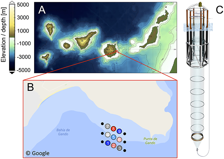
Figure 1. (A) Bathymetric map of the Canary Islands archipelago. Visualization based on data from GEBCO, British Oceanographic Data Centre (Weatherall et al., 2015). (B) Close-up of the study site in Gando Bay (GPS coordinates: 27° 55′ 41″ N, 15° 21′ 55″ W), including mesocosm arrangement and mooring (not to scale). Numbers in the circles indicate mesocosm ID and colors represent CO₂ treatment (see Table 1). Source: Google Maps. (C) Schematic illustration of a mesocosm unit. The bag has a diameter of 2 m and reaches 13 m below the water surfaces. The attached sediment trap extends the mesocosm to a depth of 15 m, thereby, enclosing a total water volume of ~35 m³ (see Table 1).

Mesocosm Setup, Deployment Procedure, and Maintenance

On September 23rd 2014, the research vessel Hesperides deployed nine “Kiel Off-Shore Mesocosms for Future Ocean Simulations” (KOSMOS, M1–M9; Riebesell et al., 2013a), which were moored in clusters of three in the northern part of Gando Bay (27° 55′ 41″ N, 15° 21′ 55″ W) at a depth of ~20–25 m (Figure 1).

Each mesocosm unit consisted of an 8 m high flotation frame, a cylindrical mesocosm bag (13 m length, 2 m diameter) made of transparent thermoplastic polyurethane foil (1 mm thick) that allows for penetration of light in the PAR spectrum, as well as a conical sediment trap (2 m long) that tightly seals the bottom of the mesocosm and allows for collection of sinking organic material with a vacuum pump system on a regular basis (Figure 1C).

The bags were folded and mounted onto the floatation frames prior to deployment. Once in the water, the bags were unfolded immediately and submerged below the water surface with the upper opening 1 m below sea surface. Both the upper and lower openings were covered with meshes (3 mm mesh size) to exclude patchily distributed nekton and large zooplankton like fish larvae or jellyfish from the enclosed water bodies. The mesocosm bags were then left floating in the water column for 4 days to allow for rinsing of the bags' interior and free exchange of plankton (<3 mm) between the mesocosms and the surrounding water. On September 27th, divers replaced the mesh at the bottom of the mesocosm bags with the sediment traps, while a boat crew simultaneously pulled the upper part of the bags above the sea surface. This step separated the water bodies within the mesocosms from the surrounding water and thus marked the start of the experiment (day −4 = t-4, Figure 2). The entire procedure lasted for <2 h, thereby minimizing differences between the enclosed water masses among mesocosms.

FIGURE 2

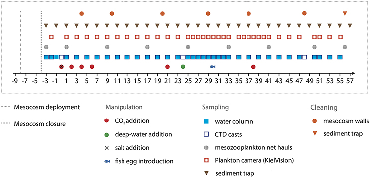
Figure 2. Timeline indicating important events, such as experimental manipulations, sampling activities, and maintenance work.

The experiment lasted for 62 days in total, starting with the closing of the mesocosms on t-4 and finishing with the last sampling of the sediment trap on t57. Day t0 (October 1st) denotes the day of the first CO₂ manipulation, corresponding to the establishment of elevated pCO₂ as the experimental treatment (see Section CO₂ Manipulation). In the fourth week of the experiment (t24), we injected deep water into the mesocosms to simulate a natural upwelling event (Section Simulated Upwelling through Addition of Deep Water). Unfortunately, one mesocosm (M6) was lost on t26, when strong currents in Gando Bay pulled some of the moorings and mesocosms ~50 m seawards. The bag of M6 was irreparably damaged during the recovery procedure. Thus, M6 was excluded from sampling and analyses after t26.

Mesocosms were cleaned from the inside and outside to minimize wall growth by benthic organisms, which would consume nutrients and eventually lead to decreasing light intensities inside the mesocosms. Therefore, mesocosm wall cleaning was conducted in regular intervals throughout the experiment (Figure 2) using a specifically designed cleaning ring for the inner surface, and scrubbers for the outside of the mesocosm bags (Riebesell et al., 2013a; Bach et al., 2016). Unfortunately, however, the conical sediment trap and parts of the lowest mesocosm segment could not be cleaned from the inside due to the narrow tapered design. These parts corresponded to ~7% of the inner surface of the mesocosm, which experienced some degree of wall growth (see Section Plankton Community Structure and Influence of Ocean Acidification).

CO₂ Manipulation

To simulate ocean acidification in our experiment, we added different amounts of CO₂-saturated seawater to the mesocosms, following the method described in Riebesell et al. (2013a). For preparation of CO₂-saturated seawater, we collected about 1,500 L of natural seawater from Melenara Bay at ~10 m depth using a pipe and pre-filtration system connected to the PLOCAN facilities. The water was aerated with pure CO₂ gas for at least 1 h until reaching saturation and pH_NBS values of ~4.7. Afterwards, the water was filtered again (20 μm) and transferred into 20 L bottles, which were then transported by boat to the mesocosm study site.

For addition of the CO₂-saturated water to the mesocosms, we used a special distribution device (“spider”) with a large number of small tubes to distribute the water uniformly within a radius of ~1 m. By constantly pulling the spider up and down inside the mesocosms, we ensured homogenous CO₂ enrichment throughout the entire water columns. By adding different amounts of CO₂-saturated seawater to seven of the nine mesocosms, we set up an initial gradient in pCO₂ from ambient levels (~400 μatm) to concentrations of ~1,480 μatm in the highest CO₂ treatment. No CO₂ water was added to mesocosms M1 and M9, which served as a control (ambient pCO₂). To avoid an abrupt disturbance of the plankton community, this initial CO₂ manipulation was carried out incrementally in four steps over a period of 7 days between t0 and t6 (Figure 2). Two further CO₂ additions were conducted during the experiment in order to account for loss of CO₂ through air-sea gas exchange. The first time was on t21 during the oligotrophic phase to adjust pCO₂ before deep water addition, and the second time on t38 in the post-bloom phase (Figure 2).

Simulated Upwelling through Addition of Deep Water

One of the major goals of this study was to investigate whether potential effects of elevated CO₂ on natural plankton communities in the study region might differ between oligotrophic conditions and during bloom situations. Such plankton blooms regularly occur in response to upwelling of deep water, which is primarily driven by mesoscale variability (e.g., eddies) and results in transport of nutrient-rich water masses from several hundreds of meters depth to the (usually) nutrient-poor surface layer (Arístegui et al., 1997; Basterretxea and Arístegui, 2000). Besides inorganic nutrients, oceanic deep water masses usually exhibit distinct signatures of minor constituents such as dissolved organic matter and trace metals, elevated pCO₂, or seeding populations of plankton species (Pitcher, 1990; Hansell et al., 2009; Aparicio-Gonzalez et al., 2012; Tagliabue et al., 2014). All of these factors may have minor or major influences on the ecosystem in the surface layer, which go beyond the effects of the major nutrients N, P, and Si. Consequently, a “simple” addition of inorganic nutrients would not be sufficient for a realistic simulation of a natural upwelling event.

To overcome this challenge, we specifically developed a deep water collection system that allowed us to obtain the large amounts of nutrient-rich deep water required for mimicking an upwelling event in our mesocosm experiment. The goal was to replace ~20% of the mesocosm volumes with deep water, thereby ensuring a sufficiently large input of inorganic nutrients comparable to those observed during natural upwelling events in the region (Arístegui et al., 1997; Neuer et al., 2007).

The flexible walls of the deep water collector consisted of fiber-reinforced food-grade polyvinyl chloride material (opaque), which was high-frequency welded into a pear-like shape with a volume of ~85 m³ (Figure 3A). The opening (diameter of ~25 cm) was equipped with a specifically-designed water intake device (based on a modified propeller drive) and a sealing disc as a closure mechanism for the deep water collector. Operation of both components was time-controlled (programmable), thereby allowing for remotely operated collection of water at a desired depth. A screen with 10 mm mesh size covered the opening to ensure that no large particles or organisms entered the deep water collector. Furthermore, a weight of ~300 kg was attached to the deflated deep water collector before deployment to submerge it in the ocean until the target depth was reached. An acoustic trigger was installed to release the weight after completion of the water intake, thereby allowing the rise of the filled deep water collector to the sea surface, only driven by the gentle buoyancy of 24 floats attached to the main frame (Figure 3B).

FIGURE 3

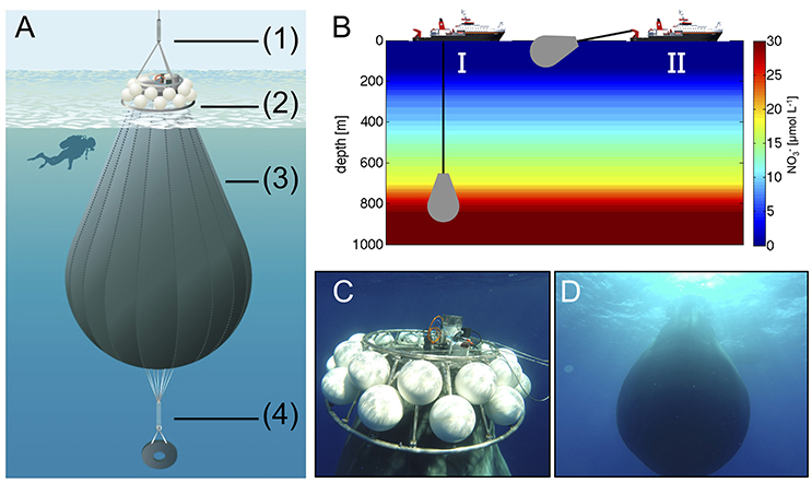
Figure 3. (A) Schematic illustration of the deep water collector, including (1) an expander for compensation of ship movement, (2) remotely-controlled filling and closing mechanism, and floatation bodies (total buoyancy ~400 kg), (3) a flexible tank welded from fiber-reinforced food-grade PVC with a volume of ~85 m³, and (4) a weight system for submersion with acoustic release trigger. Illustration by R. Erven. (B) Ship-operated collection of nutrient-rich deep water with the custom-designed system (I) and towing of the bag to the study site (II). (C,D) Underwater photographs of the deep water collector after successful deployment (Pictures taken by the KOSMOS dive team).

On October 23rd (t22), we transported the deep water collection system to a location about 4 nautical miles north-east from the study site, where water depth was ~1,000 m and thus sufficiently deep for deployment. Transport and operation of the deep water collector was carried out with the vessel “SAPCAN IV” (chartered from Amadores harbor service, Las Palmas). Upon arrival at the target location, the deep water collector was lowered to a depth of ~650 m, where ~85 m³ of water were collected Figures 3C,D. After resurfacing of the collector, it was gently towed back to the study site, where it was anchored until addition to the mesocosms 2 days later on t24. In the meantime, defined amounts of water had to be removed from the mesocosms to create space for subsequent addition of deep water. To accomplish this, we used a submersible pump (Grundfos SP-17-5R) to remove known volumes of water from the mesocosms at ~5 m depth on October 24th (t23).

In order to reach the desired mixing ratio of deep water of about 20%, a total of ~75 m³ of deep water were distributed among the nine mesocosms. Before addition, we characterized the deep water biologically and chemically by the full set of variables also routinely sampled in the mesocosms (see Table 2). Since deep water addition had to be carried out for each mesocosm separately one after another, we anticipated that this procedure would last at least several hours. To minimize nutrient uptake and growth by phytoplankton during this time, we conducted the deep water addition during night time, thus ensuring identical starting conditions of all mesocosms for the following experimental phase. Accordingly, deep water was added in two steps during the night of October 25th–26th (t24–t25), lasting for ~9 h in total.

The actual transfer of deep water to the mesocosms was conducted by submerging a pump (the same as for water removal described above) into the deep water collector and pumping the water into the mesocosms with an injection device similar to the “spider” used for CO₂ additions (see above), but with larger tube diameters and larger volume throughput. Continuous up and down movement of this enlarged spider during addition ensured homogenous vertical distribution of deep water inside the mesocosms. In the first step, we added ~80% of the calculated amount of deep water to each mesocosm. Since the salinity of the deep water was much lower than in the mesocosms (35.7 vs. 37.7), the mixing ratio of mesocosm water with deep water could be calculated from precisely measured changes in salinity. Based on CTD profiles and salinity calculations immediately after the first deep water addition, the second addition was then used for fine-tuning and adjustment of all mesocosms to identical deep water mixing ratios and concentrations of inorganic nutrients. Furthermore, by adding defined amounts of deep water with known salinity, and measuring the resultant salinity change in the mesocosms, we could accurately estimate the total volume of seawater in each mesocosm enclosure. The volumes determined by this method were ~35 m³ on average (±5%, see Table 1).

TABLE 1

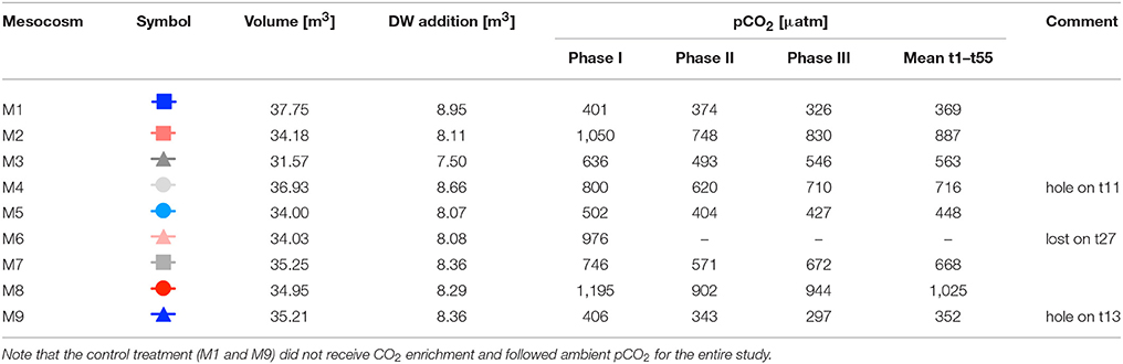
Table 1. Mesocosm experimental setup, including symbols and color-code for other figures, mesocosm volumes right before deep water addition, amount of deep water (DW) added to each mesocosm, and average pCO₂ values during different phases of the experiment (see Section Oligotrophic Phase and Plankton Bloom in Response to Deep Water Addition for definition of phases).

Addition of Fish Larvae

One of our study objectives was to investigate how effects of OA on plankton communities might propagate to higher trophic levels. Accordingly, we added ~330 eggs of greater amberjack (Seriola dumerili) to each mesocosm on October 31st (t30), which was during the time of peak biomass after deep water addition on t24. The number of added eggs was determined as a trade-off between preventing potential top-down effects from becoming too strong on the one hand, and providing the presence of sufficient fish for sampling (based on expected survival) on the other hand. Eggs of greater amberjack were collected from existing broodstock, hold by the Aquaculture research group (GIA) of the University of Las Palmas de Gran Canaria (ULPGC). All protocols within the breeding facilites were approved within the EU project “AQUAEXCELL” (ethics permit number: OEBA-ULPGC04/2016). The fish eggs were gently introduced by submerging the brood containers inside the mesocosms (~3 m depth) from day t30 until t32, with calculated time of hatching at 2 days after introduction.

Unfortunately, it was not possible to determine the abundance of fish larvae on a continual basis. No larvae of S. dumerili could be found in the net catches, possibly due to their escape from the towed net. Deployment of light traps was not successful either. Some dead fish larvae were found by screening the sediment trap material on the days after hatching. While this approach did not provide robust quantitative estimates, e.g., due to the fragility and rapid decay of dead organisms, it indicated substantial mortality of fish larvae within the first few days after hatching. Furthermore, no live individuals were found in the final sampling (t56) with a 1 mm net that covered the full diameter of the mesocosms, indicating that there was no survival of fish larvae until the end of the experiment. Nevertheless, it should be kept in mind that fish larvae might have had a top-down effect on the plankton communities in the mesocosms after ~t32, even though this possible influence is most likely negligible.

Sampling Procedures and CTD Operations

We conducted out a comprehensive sampling effort for a wide range of physical, ecological, and biogeochemical variables in the mesocosms and the surrounding waters on every second day, usually lasting from 9 a.m. until noon. An exception was the period right after deep water addition (t25–t33), when a rapid response of the plankton community was observed, and most variables were sampled on a daily basis.

Our preferred method of sample collection in mesocosm studies involves use of depth-integrating water samplers (IWS, HYDRO-BIOS, Kiel), which gently take in a total volume of 5 L uniformly distributed over the desired depth. However, this method is rather time-consuming, with one IWS haul usually lasting 3–4 min. Because the sample volume of oligotrophic water required for filtrations, incubations, etc., usually amounted to at least 60–70 L per mesocosm per day, we decided to adjust our sampling strategy and applied two methods of water collection in parallel, depending on the requirements of the various measurement variables (Table 2).

TABLE 2

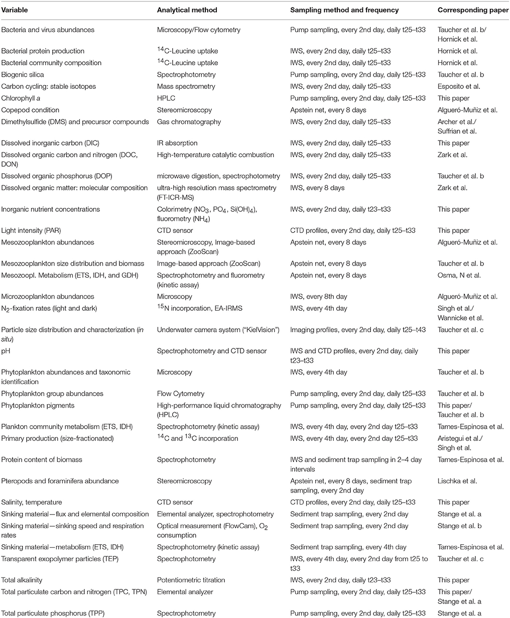
Table 2. Overview of measured variables in the experiment, including the analytical method, sampling method, and frequency, as well as corresponding papers providing an in-depth analysis of respective variables.

For variables that are sensitive to gas exchange or contamination, we collected integrated water samples using the IWS over 0–13 m water depth and directly filled subsamples into separate containers on the sampling boats following the specific requirements and protocol for the respective variable (see Section Data Analysis and Statistics). These sensitive variables were dissolved inorganic carbon (DIC), pH, dimethyl sulfide (DMS), inorganic nutrients [nitrate (${\text{NO}}_3^{-}$), nitrite (${\text{NO}}_2^{-}$), dissolved silicate (Si(OH)₄), ammonium (${\text{NH}}_4^{+}$), phosphate (${\text{PO}}_4^{3-}$)], dissolved organic carbon, nitrogen, and phosphorus (DOC, DON, DOP), and water for all in vitro incubation experiments such as primary production (¹³C and ¹⁴C), N₂-fixation, bacterial degradation of sinking organic matter, or bacterial protein production assays.

Samples for other variables (e.g., particulate organic matter) were obtained with a custom-built pump system that allowed for a much faster collection of large sampling volumes. The system consisted of a manually operated pump, a 20 L carboy, a valve with integrated pressure gauge that connected to a 20 m long plastic tube (25 mm diameter), and a special inlet with several water intakes mounted to the open end of the tube. By applying the pump, a gentle vacuum was created (<150 mbar) in order to suck in water from the mesocosms into the tube and carboy. By moving the tube and attached inlet up and down during pumping (0–13 m), integrated water samples similar to the ones obtained by the IWS could be collected. To achieve this, pumping rate and vertical movement were synchronized with the holding capacity of the sampling carboy in order to avoid overflow of water before the sample could be considered integrated, i.e., before the vertical profile was completed. The 20 L sample carboys were then stored protected from direct sunlight on deck of the boats until sampling was completed. Once on shore, the samples were stored in a dark and temperature-controlled room (set to 16°C) where subsamples were taken for a variety of ecological and biogeochemical measurements (Table 2).

Sinking particulate matter was collected in the sediment traps at the bottom of the mesocosms. Sampling of the sediment traps was carried out every second day throughout the entire study, using a vacuum system connected to the tubes, which were attached to the collection cups following Boxhammer et al. (2016).

Mesozooplankton samples were acquired with an Apstein net (55 μm mesh size, 0.17 m diameter opening) in 8-day intervals. The maximum sampling depth of net tows was 13 m to avoid contact of the Apstein net with the sediment trap material, thus resulting in an overall sampling volume of ~295 L per net tow. Mesozooplankton samples were kept dark and cool until transport to shore, where they were preserved with sodium tetraborate-buffered formalin (4% v/v) for counting and taxonomic analyses. The number of zooplankton net catches per sampling day was restricted to every 8 days to avoid “overfishing,” i.e., exerting a too strong influence on top-down control of the system by removing zooplankton biomass.

CTD casts were carried out with a hand-held self-logging CTD probe (CTD60M, Sea and Sun Technologies) in each mesocosm and in the surrounding water on every sampling day. Thereby we obtained vertical profiles of temperature, salinity, pH, dissolved oxygen, chlorophyll a, and photosynthetically active radiation (PAR). Technical details on the sensors and data analysis procedures are described by Schulz and Riebesell (2013). Potentiometric measurements of pH_NBS (NBS scale) from the CTD were corrected to pH_T (total scale) by daily linear correlations of mean water column potentiometric pH_NBS to pH_T as determined from carbonate chemistry.

Sample Processing, Measurements, and Analysis

Carbonate Chemistry

Samples for dissolved inorganic carbon (DIC) and total alkalinity (TA) were gently sterile-filtered (0.2 μm pore size) using a peristaltic pump and stored at room temperature until measurement on the same day.

DIC concentrations were determined by infrared absorption using a LI-COR LI-7000 on an AIRICA system (MARIANDA, Kiel). Measurements were made on three replicates, with overall precision typically being better than 5 μmol kg⁻¹. TA was analyzed by potentiometric titration using a Metrohm 862 Compact Titrosampler and a 907 Titrando unit following the open-cell method described in Dickson et al. (2003). The accuracy of both DIC and TA measurements was determined by calibration against certified reference materials (CRM batch 126), supplied by A. Dickson, Scripps Institution of Oceanography (USA).

Other carbonate chemistry variables such as pCO₂, pH (on the total scale: pH_T), and aragonite saturation state (Ω_aragonite), were calculated from the combination of TA and DIC using CO2SYS (Pierrot et al., 2006) with the carbonate dissociation constants (K₁ and K₂) of Lueker et al. (2000).

Inorganic Nutrients

Samples for inorganic nutrients were collected in acid-cleaned (10% HCl) plastic bottles (Series 310 PETG), filtered (0.45 μm cellulose acetate filters, Whatman) directly after arrival of water samples in the laboratory, and analyzed on the same day to minimize potential changes due to biological activity. ${\text{NO}}_3^{-}$ + ${\text{NO}}_2^{-}$ (=${\text{NO}}_3^{-}$/${\text{NO}}_2^{-}$), Si(OH)₄, and ${\text{PO}}_4^{3-}$ concentrations were measured with a SEAL Analytical QuAAtro AutoAnalyzer connected to JASCO Model FP-2020 Intelligent Fluorescence Detector and a SEAL Analytical XY2 autosampler. AACE v.6.04 software was used to control the system. The measurement approach is based on spectrophotometric techniques developed by Murphy and Riley (1962) and Hansen and Grasshoff (1983). Ammonium concentrations were determined fluorometrically following Holmes et al. (1999). Refractive index blank reagents were used (Coverly et al., 2012) in order to quantify and correct for the contribution of refraction, color, and turbidity on the optical reading of the samples. Instrument precision was calculated from the average standard deviation of triplicate samples [±0.007 μM for ${\text{NO}}_3^{-}$/${\text{NO}}_2^{-}$, ±0.003 μM for ${\text{PO}}_4^{3-}$, ±0.011 μM for Si(OH)₄, and ±0.005 μM for ${\text{NH}}_4^{+}$]. Detection limits for the different nutrients were 0.03 (${\text{NO}}_3^{-}$/${\text{NO}}_2^{-}$), 0.008 (${\text{PO}}_4^{3-}$), 0.05 (Si(OH)₄), and 0.01 (${\text{NH}}_4^{+}$) μmol L⁻¹. Analyzer performance was controlled by monitoring baseline, calibration coefficients, and slopes of the nutrient species over time. The variations observed throughout the experiment were within the analytical error of the methods.

Chlorophyll a and Phytoplankton Pigments

Samples for chlorophyll a (chl-a) and other phytoplankton pigments were analyzed by reverse-phase high-performance liquid chromatography (HPLC, Barlow et al., 1997) following collection by gentle vacuum filtration (<200 mbar) onto glass fiber filters (GF/F Whatman, nominal pore size of 0.7 μm) with care taken to minimize exposure to light during filtration. Samples were retained in cryovials at −80°C prior to analysis in the laboratory. For the HPLC analyses, samples were extracted in acetone (100%) in plastic vials by homogenization of the filters using glass beads in a cell mill. After centrifugation (10 min, 5,200 rpm, 4°C) the supernatant was filtered through 0.2 μm PTFE filters (VWR International). From this, phytoplankton pigment concentrations were determined by a Thermo Scientific HPLC Ultimate 3,000 with an Eclipse XDB-C8 3.5 u 4.6 × 150 column. Contributions of individual phytoplankton groups to total Chl-a were then estimated using the CHEMTAX software, which classifies phytoplankton based on taxon-specific pigment ratios (Mackey et al., 1996). Furthermore, phytoplankton samples for microscopy were obtained every 4 days, fixed with acidic Lugol solution and analyzed using the Utermöhl technique (Utermöhl, 1931), with classification until the lowest possible taxonomical level.

Particulate Matter

Samples for particulate carbon and nitrogen (TPC/TPN) were filtered (<200 mbar) onto pre-combusted GF/F glass fiber filters (450°C for 6 h; Whatman 0.7 μm nominal pore size). Afterwards, sample filters were dried (60°C) overnight and wrapped in tin foil until analysis. Concentrations of carbon and nitrogen were measured on an elemental CN analyzer (EuroEA) following Sharp (1974). Note that for particulate carbon, one out of three replicate TPC filters per sample was fumed with hydrochloric acid (37%) for 2 h before measurement in order to remove particulate inorganic carbon (PIC) and thereby allowing us to distinguish between inorganic and organic forms of particulate carbon (Bach et al., 2011). Comparison of TPC and POC (particulate organic carbon) indicated that PIC was virtually absent in the seawater during our study, i.e., TPC was constituted almost entirely of POC.

Zooplankton Community Composition

Microzooplankton samples were obtained every 8 days, immediately fixed after sub-sampling with acidic Lugol solution and stored in 250 mL brown glass bottles until analysis using the Utermöhl technique (Utermöhl, 1931). In the scope of this study we distinguished between ciliates and heterotrophic dinoflagellates.

Abundances of mesozooplankton (mostly copepods and appendicularia) from net haul samples (>55 μm, every 8 days) were counted using a stereomicroscope (Olympus SZX9) and classified until the lowest possible taxonomical level.

Data Analysis and Statistics

To identify potential ecological effects of CO₂ on the composition of the plankton community, we carried out multivariate analysis for abundance data of the different plankton groups. Therefore, we calculated the average abundances of different plankton groups during three experimental phases: (I) the oligotrophic phase until t23, (II) the phytoplankton bloom between t25 and t35, and (III) the post-bloom phase from t37 until the end of the study. All phytoplankton data used are from HPLC and CHEMTAX analysis, whereas numbers for micro- and meso-zooplankton were obtained by microscopy. In total, we distinguished 13 plankton functional groups that we used for analysis in the present study.

To account for the different scales of abundance of the various plankton groups, ranging from picophytoplankton (<2 μm) to mesozooplankton larger than 1 mm, all abundance data were normalized by their range as:

$\begin{array}{cc}\begin{array}{c}{\text{N}}_{\text{norm}} = \text{N}/\left({\text{N}}_{\text{max}}-{\text{ N}}_{\text{min}}\right)\end{array}& \left(1\right)\end{array}$

where N is the abundance of each individual group, and N_min and N_max refer to the highest and lowest values found in the nine mesocosms. Thereby, all data are scaled to a range between 0 and 1, while maintaining the overall sample variance, as well as the relative differences between mesocosms.

After normalization of raw data, we generated ecological distance matrices using Bray–Curtis dissimilarity, which were then used for all multivariate analyses conducted here. In a first step, we performed non-metric multidimensional scaling (NMDS) to visualize ordination of the plankton communities in the mesocosms in response to CO₂ in the different experimental phases.

For a more quantitative assessment of how CO₂ might have influenced plankton community structure, we investigated the relationship between ecological distance (Bray–Curtis dissimilarity) and environmental distance, in this case pCO₂ (using Euclidian distance). Therefore, we applied a linear regression model to environmental and ecological distance data, using the same data matrices and phases as described above for the NMDS approach. Thus, every data point in the regression analyses corresponds to a pair-wise comparison of mesocosms with respective environmental distance (differences in pCO₂) and ecological distance (Bray–Curtis dissimilarity). The latter was calculated using the same (normalized) abundance data from plankton groups as for the NMDS analysis. This method allowed us to detect whether differences in plankton community composition were related to pCO₂. A statistically significant relationship between CO₂ and plankton community composition was assumed for p < 0.05 in the linear regression. The Mantel Test serves to ensure that these patterns did not arise by chance (when p < 0.05). All multivariate statistical analysis were conducted with the Fathom Toolbox for MATLAB (Jones, 2015).

Results and Discussion

Environmental Boundary Conditions

Environmental conditions in Gando Bay during the mesocosm experiment were typical for late summer/early fall in the study region. Average temperatures in the mesocosms slightly decreased from ~24.4 to 22.3°C over the course of the study, corresponding to decreasing air temperatures during early autumn (Figure 4, Supplementary Material). Vertical profiles of temperature and salinity from the CTD showed a uniform distribution of both variables, indicating that there was no stratification and that the water columns in the mesocosms were well-mixed throughout the entire study period (Figure 4). Temperature profiles of the surrounding waters in Gando Bay were very similar to those in the mesocosms.

FIGURE 4

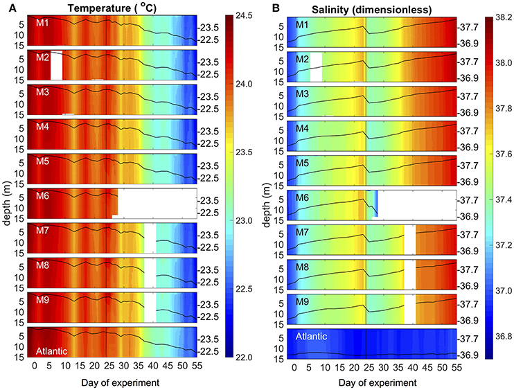
Figure 4. Vertical profiles of temperature (A) and salinity (B) in the mesocosms (M1–M9) and the surrounding Atlantic over the course of the study. Average values over the entire water column are represented by the black lines on top of the colored contours, including the corresponding additional y-axes on the right side of the boxes. The vertical black line on t24 denotes deep water addition into the mesocosms.

Average salinity in the mesocosms steadily increased from ~36.95 to 38.05 during the experimental period, interrupted only by a decrease due to addition of (less saline) deep water on t24 (Figure 4). The salinity increase was driven by evaporation, which was substantial due to relatively high temperatures and usually windy conditions (see Supplementary Material). In contrast, salinity in the surrounding waters remained almost constant throughout the experimental period. Because of this salinity difference, we could easily detect the presence of holes due to damaged mesocosm walls based on daily changes in salinity: When lower salinity water from the surrounding water entered the mesocosms, the daily increase in salinity of a particular mesocosm was lower than in the other mesocosms. Based on these observations, we could observe that M4 and M9 had holes around t11 (M4) and t13 (M9). Divers sealed the holes immediately after detection, by gluing small rubber patches onto the outside of the mesocosm bags.

To what extent these water intrusions might have affected the composition of the plankton communities in the mesocosms is difficult to assess, especially since they occurred during the oligotrophic phase when plankton abundances were low and measurement variability was comparably high. However, we did not observe anomalies in any of the measured variables during or after these damages. Furthermore, neither M4 nor M9 displayed any fundamental differences in plankton community composition or succession patterns throughout the rest of the study. Thus, we are confident that the temporal water intrusions through the holes only had a minor influence on the results presented here.

Carbonate Chemistry and Simulated Ocean Acidification

The injection of different amounts of CO₂-enriched seawater into the mesocosms in the period between t0 and t6 elevated DIC concentrations from initial values of ~2,079 up to 2,342 μmol kg⁻¹ in the highest CO₂treatment (M8). The corresponding increase in pCO₂ resulted in a treatment gradient ranging from 410 to 1414 μatm after the initial CO₂ enrichment (t7, Figure 5).

FIGURE 5

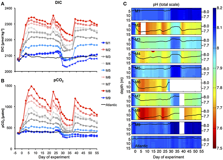
Figure 5. Carbonate chemistry. Temporal development of average DIC (A) and pCO₂ (B), as well as vertical profiles of pH (C) during the experiment. Style and color-coding in panel A+B are given in Table 2.

Afterwards, pCO₂ in the mesocosms decreased quite rapidly due to gas exchange at the air-sea interface. Although, we did not carry out direct measurements of gas exchange, the rapid decreases in pCO₂ and DIC until t20 were not reflected in build-up of total particulate carbon (TPC, Figure 7C), suggesting that the loss of inorganic carbon can be attributed predominantly to outgassing of CO₂. This is consistent with theoretical considerations, which suggest that rates of gas exchange should be high under the environmental conditions during our study, i.e., relatively high water temperatures, high wind speeds, and constant convective mixing of the entire water column in the mesocosms (Smith, 1985; Jähne et al., 1987). During the plankton bloom between t25 and t35 (see Section Oligotrophic Phase and Plankton Bloom in Response to Deep Water Addition), the decline in DIC concentrations was further enhanced by photosynthetic CO₂ fixation.

To compensate for the loss of CO₂ and readjust the treatment gradient, we conducted two more CO₂ enrichments on t21 and t38 (Figure 5). Altogether, the CO₂ gradient could be maintained reasonably well throughout the entire study. Furthermore, vertical profiles of pH show that carbonate chemistry conditions were distributed equally over the depth of the mesocosms, ensuring that all organisms in the water column experienced similar CO₂ conditions (Figure 5C).

Oligotrophic Phase and Plankton Bloom in Response to Deep Water Addition

Oligotrophic Phase

During the first few weeks of the experiment, we observed typical oligotrophic conditions in the mesocosms. Concentrations of all inorganic nutrients were very low and relatively constant. Average concentrations of ${\text{NO}}_3^{-}+$${\text{NO}}_2^{-}$, ${\text{PO}}_4^{3-}$, and Si(OH)₄ until t23 were 0.06 ± 0.01, 0.026 ± 0.004, and 0.26 ± 0.04 μmol L⁻¹, respectively (Figure 6). These values are within the range of observations for oligotrophic conditions in this region (Neuer et al., 2007). Correspondingly, chlorophyll a concentrations were very low, amounting to ~0.1 μg L⁻¹ on average until t23 (Figure 7A). Despite these low nutrient concentrations, chl-a slightly increased from ~0.05 to 0.13 μg L⁻¹ between t1 and t11 (Figure 7B).

FIGURE 6

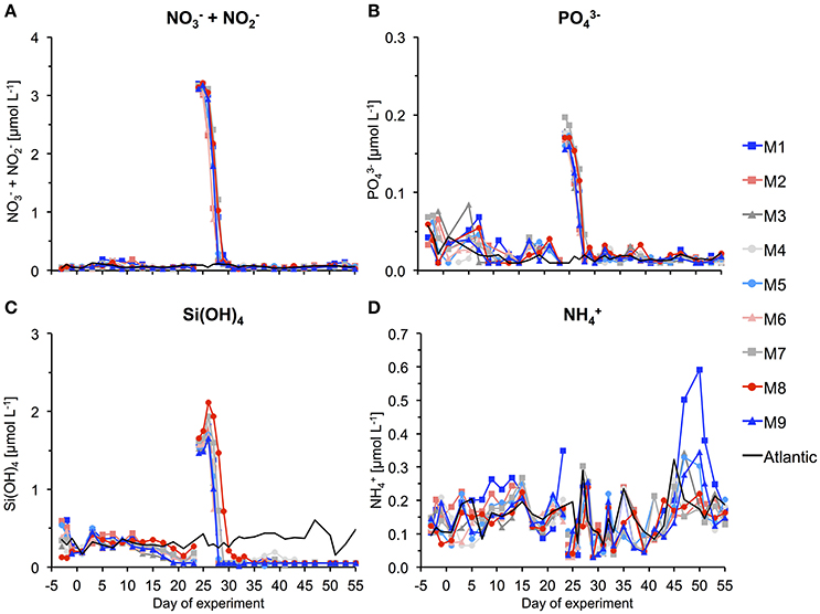
Figure 6. Inorganic nutrient concentrations over the course of the study. The gap and associated change in concentrations between t23 and t25 denotes addition of nutrient-rich deep water to the mesocosms. (A) Nitrate and nitrite, (B) phosphate, (C) silicate, and (D) ammonium.

FIGURE 7

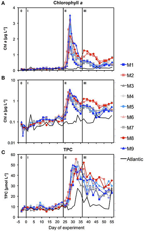
Figure 7. (A) Temporal development of chlorophyll a concentrations in the mesocosms and the surrounding waters. Black lines and roman numbers indicated the different phases of the experiment. (B) Same as in (A) but with log-scaled y-axis. (C) Total particulate carbon.

Between t16 and t22, easterly winds transported dust from the Sahara desert to the Canary Islands and the experiment site. Such dust events regularly occur in the study area and can sometimes constitute a considerable source for input of trace nutrients, such as iron (Gelado-Caballero et al., 2012). The total dry deposition flux from t16 to t22 was estimated at ~230 mg m⁻², which is comparable to other weak dust events in the region (Gelado-Caballero, Personal Communication). Is noteworthy that some nutrients displayed changes that coincided with the period of dust deposition. Si(OH)₄ concentrations began to decrease slightly until t23, and ${\text{NH}}_4^{+}$ also decreased between t15 and t19. While it is possible that this was at least partly driven by stimulation of phytoplankton growth in response to dust deposition, a closer look at the temporal development of chl-a indicates that growth began in fact much earlier (from t1 onwards, Figure 7B). Thus, we conclude that dust deposition did most likely not have a major effect on the phytoplankton communities in our experiment.

Deep Water Addition and Phytoplankton Bloom

On day t22, we collected ~85 m³ of oceanic deep water with inorganic nutrient concentrations of 16.7, 1.05, and 7.46 μmol L⁻¹ for ${\text{NO}}_3^{-}+$${\text{NO}}_2^{-}$, ${\text{PO}}_4^{3-}$, and Si(OH)₄, respectively. After injection of known volumes of deep water into the mesocosms in the night from day t24 to t25, inorganic nutrients were elevated to concentrations of ~3.15, 0.17, and 1.60 μmol L⁻¹ for ${\text{NO}}_3^{-}+$${\text{NO}}_2^{-}$, ${\text{PO}}_4^{3-}$, and Si(OH)₄, respectively (Figure 6, Table 3).

TABLE 3

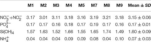
Table 3. Inorganic nutrient concentrations in the mesocosms after deep water addition (t25).

Chl-a concentrations increased rapidly in response to supply of inorganic nutrients from the deep water addition. Maximum values were reached on t28 in all mesocosms, being elevated by more than 25-fold compared to oligotrophic conditions before the bloom (Figures 7A,B). Correspondingly, inorganic nutrients were depleted quickly, reaching values close to detection limit between t28 and t30 (Figure 6).

After the bloom peak, chl-a declined rapidly until t35, when it even started to increase again slightly in some of the mesocosms (M2, M8). Afterwards, chl-a levels displayed some fluctuations with an overall decreasing tendency until the end of the study. Yet, concentrations remained clearly elevated compared to oligotrophic conditions before the bloom.

Particulate Carbon

The proportional increase of TPC concentrations after deep water addition was similar to that of chlorophyll a during the phytoplankton bloom (Figure 7C). However, the decline of TPC after the bloom peak was much slower and concentrations remained at levels much higher than before the bloom, suggesting that a large portion of biomass generated by phytoplankton was retained in the water column, e.g., by being transferred into heterotrophic biomass or by accumulating as detritus with close to neutral buoyancy (mucus-rich aggregates/marine snow).

Definition of Experimental Phases

Based on the timing of deep water addition and the temporal development of chlorophyll a concentrations described above, we define three major experimental phases (Figure 7A): The oligotrophic phase (I) from t1 until t23 covers the entire period of low chl-a concentrations before addition of deep water on t24. Phase II lasts from t25 to t35 and encompasses the entire bloom event that occurred in response to deep water addition. This includes both the major chl-a build-up until t28 as well as the subsequent bloom decline until t35, when the decrease in chl-a stopped. The post-bloom phase (III) covers the entire remaining period from t37 until the end of the experiment on t57. Note that phase 0 includes baseline data from the time before the first CO₂ manipulation (t-3 and t-1) and was thus excluded from statistical analysis of CO₂ effects.

Plankton Community Structure and Influence of Ocean Acidification

During the oligotrophic phase, the phytoplankton community was dominated by small phytoplankton, mostly consisting of cyanobacteria (Synechococcus), which constituted 70–80% of chlorophyll a (Figure 8). This picture changed in phase II, when deep water addition resulted in a pronounced phytoplankton bloom that was dominated by diatoms, accounting for >70% of total chlorophyll a. Microscopic analysis revealed that the dominant species were relatively large chain-forming diatoms such as Leptocylindrus sp., Guinardia sp., and Bacteriastrum sp., but also detected other species such as Nitzschia sp. at lower abundances. The remaining phytoplankton consisted mainly of dinoflagellates, Dictyocha-like flagellates (belonging to chrysophytes) in some mesocosms, and prymnesiophytes (mostly Phaeocystis sp.) throughout the experiment (Figure 8).

FIGURE 8

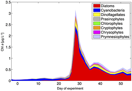
Figure 8. Phytoplankton community composition from HPLC and CHEMTAX analysis (average of all mesocosms).

Microzooplankton communities in the mesocosms were mainly composed of ciliates and heterotrophic dinoflagellates, whereas mesozooplankton was dominated by different copepod species and nauplii, but also included other functional groups such as appendicularia (Algueró-Muñiz et al., in preparation).

It should be noted that underwater video footage indicated the formation of some patchy benthic growth on parts of the inner mesocosm surfaces, which could not be cleaned (i.e., the conical sediment trap and parts of the lowest mesocosm segment, see Section Mesocosm Setup, Deployment Procedure, and Maintenance). Pigment analysis of this organic material suggested that it consisted to a large part of Phaeocystis colonies. In fact, adhesion to surfaces and subsequent rapid colony formation is characteristic for Phaeocystis (Rousseau et al., 2007). However, since the affected area was rather small compared to the mesocosm volume (~10 m² uncleaned mesocosm wall surface vs. 35 m³ mesocosm volume), we are confident that this wall growth did not significantly affect the results for phytoplankton community composition and biogeochemistry presented in this study.

Altogether, the phytoplankton succession pattern observed in our mesocosms—switching from prevalence of picoeukaryotes and picocyanobacteria (Synechococcus) toward a system dominated by large diatoms and dinoflagellates—is typical for the transition from open ocean gyres to coastal upwelling regions, as well as for the species succession in mesoscale eddies (Arístegui et al., 2004; Brown et al., 2008).

The main objectives of our mesocosm campaign were to investigate (a) how ocean acidification could change plankton community composition and food-web structure in oligotrophic environments, and (b) if such potential changes might amplify or weaken during periodic upwelling events of nutrient-rich deep water. In the present paper we assess how increasing CO₂ could affect the structure of plankton community as a whole. Therefore, we included and analyzed data from different functional groups of plankton, but did not investigate patterns within these groups at more taxonomic detail, e.g., on the species level. Such questions will be investigated in more targeted studies presented within the framework of this Research Topic (Table S1).

Our analysis at the level of functional groups revealed a significant effect of CO₂ on plankton community structure, both under oligotrophic conditions (phase I) and throughout the bloom induced by simulated upwelling of deep water (phases II and III). NMDS spaces (Figure 9) show the ordination of the mesocosms according to differences in their plankton community composition. The NMDS analysis of the different phases suggests the emergence of clear differences in plankton community structure, resulting in ordination of mesocosms according to the CO₂ treatment. Notably, these differences are not attributable to the response of only one or two dominant species, but emerged from overall shifts across the entire plankton community, including various groups of phytoplankton, micro- and meso-zooplankton (Figure 9). Particularly during the bloom (phase II) and post-bloom (phase III), the two highest CO₂ mesocosms (M2, M8) appear strongly separated from the others (Figures 9B,C).

FIGURE 9

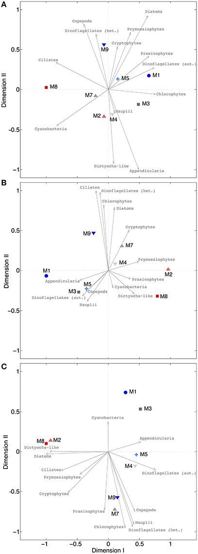
Figure 9. NMDS plots for different phases. (A) Oligotrophic phase (final stress = 0.0079), (B) plankton bloom (final stress = 0.0004), (C) post-bloom phase (final stress = 0.0221). Since all stress values are <0.1, it can be assumed that all configurations show actual dissimilarities among plankton communities in the mesocosms. Arrows indicate the role of the various plankton groups in ordination of the mesocosms.

More detailed analyses of the multivariate ecological datasets reveal a significant correlation between environmental distance (i.e., differences in pCO₂) and dissimilarity among plankton communities in the mesocosms throughout the entire study (Figure 10). During the initial oligotrophic phase (A), the plankton communities in the mesocosms were generally very similar to each other (low ecological distance between 0.1 and 0.2). However, the significant positive correlation between pCO₂ (distance) and ecological distance indicates that differences between plankton communities were larger at increasing differences in pCO₂ (Figure 10A, Table 4). In other words, differences in community composition were significantly related to differences in pCO₂ already during oligotrophic condition. These findings suggest that restructuring of plankton communities can occur under prolonged low-nutrient conditions, where observed variability in biomass is generally low. This conclusion is in line with recent studies in different oceanic regions, which reported most prominent effects of OA when inorganic nutrients were depleted (Paul et al., 2015; Sala et al., 2015; Bach et al., 2016). However, our study is the first to demonstrate this for oligotrophic waters of the subtropical North Atlantic.

FIGURE 10

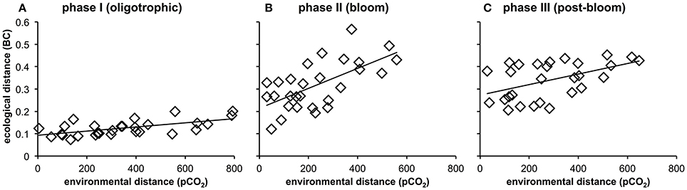
Figure 10. Relationship between environmental distance (difference in pCO₂) and ecological distance (difference in plankton community composition) in the mesocosms during the oligotrophic phase (A), the deep water induced phytoplankton bloom (B), and the post-bloom phase (C). Correlations were significant for all experimental phases (p < 0.05, n = 56, Table 4). See Methods (Data Analysis and Statistics) for more detailed information on the statistical analysis.

TABLE 4

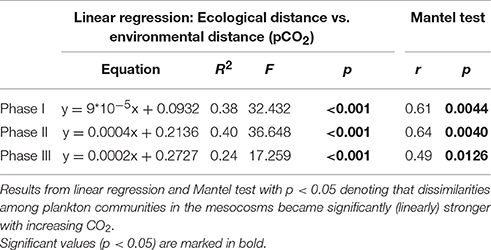
Table 4. Linear regression of ecological vs. environmental distance.

Interestingly, the magnitude of the pCO₂ effect on community structure became even larger during the bloom, displaying a much more distinct influence of pCO₂ on plankton community structure as visible by a much steeper slope of the correlation in Figure 10B (also see Table 4). This finding suggests that rather subtle changes in community composition arising under oligotrophic conditions can be amplified during productive phases in response to upwelling events, resulting in pronounced differences in succession patterns and food-web structure under high CO₂ conditions. The correlation between environmental distance (pCO₂) and ecological dissimilarity (community structure) was still visible, but weaker, during the post-bloom phase (Figure 10C). This might be explainable by the overall increase in variability among mesocosms, which is indicated by the generally higher ecological distance of ~0.3–0.4 even at low pCO₂ differences. Although, the correlation between environmental distance (pCO₂) and ecological dissimilarity (community structure) weakened during the post-bloom phase (Figure 10C), the CO₂ effect became visible in bulk variables such as chl-a or particulate carbon during this period (Figure 7). These effects are mostly driven by the two mesocosms with highest CO₂ concentrations (M2, M8), which also appear notably separated in the NMDS space during phase II and III (Figures 9B,C).

Evaluation of Simulated Upwelling of Deep Water

The results presented in the previous sections indicated a successful deep water addition to the mesocosms that broadly resembled natural upwelling events and associated phytoplankton blooms in the study region. Compared to field observations of nutrient and chlorophyll during upwelling-induced blooms in the Canary Islands region, nutrient inputs as well as rate and magnitude of biomass accumulation in our experiment were slightly elevated (Arístegui et al., 1997; Garcia-Munoz et al., 2004; Neuer et al., 2007; Lathuiliere et al., 2008).

These differences likely arise from diverging modes of deep water input between our experiment and the real ocean. Eddy-induced upwelling of deep water around the Canary Islands occurs gradually over several days or weeks, thereby constantly mixing nutrient-rich deep water with nutrient-depleted surface water (Arístegui et al., 1997; Sangra et al., 2005, 2009). In our experiment, deep water was injected in a pulsed manner (i.e., within a few hours). This created a nutrient increase that was somewhat stronger than usually observed during natural eddy-driven upwelling events in the study region. In a broader sense, these different modes of deep water input between our mesocosm experiment and eddy-induced upwelling in the real ocean can be considered analogous to batch cultures and chemostat approaches in laboratory studies, respectively.

We cannot exclude the possibility that differences between pulsed and prolonged-diluted nutrient supply could alter the build-up rates and magnitude of biomass accumulation, and thereby possibly also community composition and biogeochemical cycling. However, since plankton community structure and species succession during our study closely resembled those during natural bloom events in the Canary Islands region (Basterretxea and Arístegui, 2000; Arístegui et al., 2004), we are confident that our findings are broadly representative for natural marine ecosystems of the study area.

Conclusion and Outlook

Our study presents the first results from an in situ mesocosm experiment, in which we investigated how ocean acidification could affect plankton communities in the oligotrophic waters of the subtropical North Atlantic. One of our particular interests was to assess whether sensitivities to elevated CO₂ might differ between oligotrophic conditions and bloom situations, which regularly develop in response to periodic upwelling of nutrient-rich deep water in the study region. Using a specifically-designed deep water collector, we obtained 85 m³ of water from 650 m depth and successfully simulated a natural upwelling event in our mesocosm experiment.

Our analysis revealed a pronounced effect of increasing CO₂ concentrations on plankton community composition in the eastern subtropical North Atlantic. Moreover, our results suggest that a CO₂-driven restructuring of plankton communities under oligotrophic conditions might further amplify in bloom situations occurring in response to upwelling of deep water. These shifts in plankton community structure might profoundly influence food-web interactions and biogeochemical cycling of subtropical ecosystems. Since oligotrophic waters of the great ocean gyres cover more than half of the global ocean surface, we conclude that future research efforts in the field of ocean acidification should increasingly focus on the possible impacts in these vast oceanic regions.

Author Contributions

Conceived and designed the experiment: UR, JT, LB, TB, JC, MS, and PS. Performed the experiment: All authors. Analyzed the data: JT, LB, TB, AN, MA, JA, ME, WG, HH, AL, JM, CS, and PS. Wrote the paper: JT with input from all co-authors.

Conflict of Interest Statement

The authors declare that the research was conducted in the absence of any commercial or financial relationships that could be construed as a potential conflict of interest.

Acknowledgments

We would like to thank the Oceanic Platform of the Canary Islands (Plataforma Oceánica de Canarias, PLOCAN) for their hospitality, magnificent support and sharing their research facilities with us. Another special thanks goes to the Marine Science and Technology Park (Parque Científico Tecnológico Marino, PCTM) and the Spanish Bank of Algae (Banco Español de Algas, BEA), both from the University of Las Palmas (ULPGC), who provided additional facilities to run experiments, measurements, and analyses.

Furthermore, we thank the captain and crew of RV Hesperides for deploying and recovering the mesocosms (cruise 29HE20140924), and RV Poseidon for transporting the mesocosms and support in testing the deep water collector during cruise POS463.

This project was funded by the German Federal Ministry of Education and Research (BMBF) in the framework of the coordinated project BIOACID—Biological Impacts of Ocean Acidification, phase 2 (FKZ 03F06550). UR received additional funding from the Leibniz Award 2012 by the German Research Foundation (DFG). Furthermore, the Natural Environment Research Council provided funding for EA and ME as part of the UK Ocean Acidification Programme (NE/H017348/1).

Members of the Gran Canaria KOSMOS Consortium

Nicole Aberle-Malzahn, Steve Archer, Maarten Boersma, Nadine Broda, Jan Büdenbender, Catriona Clemmesen, Mario Deckelnick, Thorsten Dittmar, Maria Dolores-Gelado, Isabel Dörner, Igor Fernández-Urruzola, Marika Fiedler, Matthias Fischer, Peter Fritsche, May Gomez, Hans-Peter Grossart, Giannina Hattich, Joaquin Hernández-Brito, Nauzet Hernández-Hernández, Santiago Hernández-León, Thomas Hornick, Regina Kolzenburg, Luana Krebs, Matthias Kreuzburg, Julia A. F. Lange, Silke Lischka, Stefanie Linsenbarth, Carolin Löscher, Ico Martínez, Tania Montoto, Kerstin Nachtigall, Natalia Osma-Prado, Theodore Packard, Christian Pansch, Kevin Posman, Besay Ramírez-Bordón, Vanesa Romero-Kutzner, Christoph Rummel, Maria Salta, Ico Martínez-Sánchez, Henning Schröder, Scarlett Sett, Arvind Singh, Kerstin Suffrian, Mayte Tames-Espinosa, Maren Voss, Elisabeth Walter, Nicola Wannicke, Juntian Xu, Maren Zark.

Supplementary Material

The Supplementary Material for this article can be found online at: https://www.frontiersin.org/article/10.3389/fmars.2017.00085/full#supplementary-material

References

Aparicio-Gonzalez, A., Duarte, C. M., and Tovar-Sanchez, A. (2012). Trace metals in deep ocean waters: a review. J. Mar. Syst. 100, 26–33. doi: 10.1016/j.jmarsys.2012.03.008

CrossRef Full Text | Google Scholar

Arístegui, J., Barton, E. D., Alvarez-Salgado, X. A., Santos, A. M. P., Figueiras, F. G., Kifani, S., et al. (2009). Sub-regional ecosystem variability in the Canary Current upwelling. Prog. Oceanogr. 83, 33–48. doi: 10.1016/j.pocean.2009.07.031

CrossRef Full Text | Google Scholar

Arístegui, J., Barton, E. D., Tett, P., Montero, M. F., Garcia-Munoz, M., Basterretxea, G., et al. (2004). Variability in plankton community structure, metabolism, and vertical carbon fluxes along an upwelling filament (Cape Juby, NW Africa). Prog. Oceanogr. 62, 95–113. doi: 10.1016/j.pocean.2004.07.004

CrossRef Full Text | Google Scholar

Arístegui, J., Hernández-León, S., Montero, M. F., and Gomez, M. (2001). The seasonal planktonic cycle in coastal waters of the Canary Islands. Sci. Mar. 65, 51–58. doi: 10.3989/scimar.2001.65s151

CrossRef Full Text | Google Scholar

Arístegui, J., Tett, P., Hernandez-Guerra, A., Basterretxea, G., Montero, M. F., Wild, K., et al. (1997). The influence of island-generated eddies on chlorophyll distribution: a study of mesoscale variation around Gran Canaria. Deep Sea Res. I Oceanogr. Res. Pap. 44, 71–96. doi: 10.1016/S0967-0637(96)00093-3

CrossRef Full Text

Bach, L. T., Riebesell, U., and Schulz, K. G. (2011). Distinguishing between the effects of ocean acidification and ocean carbonation in the coccolithophore Emiliania huxleyi. Limnol. Oceanogr. 56, 2040–2050. doi: 10.4319/lo.2011.56.6.2040

CrossRef Full Text | Google Scholar

Bach, L. T., Taucher, J., Boxhammer, T., Ludwig, A., Achterberg, E. P., Algueró-Mu-iz, M., et al. (2016). Influence of ocean acidification on a natural winter-to-summer plankton succession: first insights from a long-term mesocosm study draw attention to periods of low nutrient concentrations. PLoS ONE 11:e0159068. doi: 10.1371/journal.pone.0159068

PubMed Abstract | CrossRef Full Text | Google Scholar

Barlow, R. G., Cummings, D. G., and Gibb, S. W. (1997). Improved resolution of mono- and divinyl chlorophylls a and b and zeaxanthin and lutein in phytoplankton extracts using reverse phase C-8 HPLC. Mar. Ecol. Prog. Ser. 161, 303–307. doi: 10.3354/meps161303

CrossRef Full Text | Google Scholar

Barton, E. D., Arístegui, J., Tett, P., Canton, M., Garcia-Braun, J., Hernández-León, S., et al. (1998). The transition zone of the Canary Current upwelling region. Prog. Oceanogr. 41, 455–504. doi: 10.1016/S0079-6611(98)00023-8

CrossRef Full Text | Google Scholar

Basterretxea, G., and Arístegui, J. (2000). Mesoscale variability in phytoplankton biomass distribution and photosynthetic parameters in the Canary-NW African coastal transition zone. Mar. Ecol. Prog. Ser. 197, 27–40. doi: 10.3354/meps197027

CrossRef Full Text | Google Scholar

Boxhammer, T., Bach, L. T., Czerny, J., and Riebesell, U. (2016). Technical note: sampling and processing of mesocosm sediment trap material for quantitative biogeochemical analysis. Biogeosciences 13, 2849–2858. doi: 10.5194/bg-13-2849-2016

CrossRef Full Text | Google Scholar

Brown, S. L., Landry, M. R., Selph, K. E., Jin Yang, E., Rii, Y. M., and Bidigare, R. R. (2008). Diatoms in the desert: plankton community response to a mesoscale eddy in the subtropical North Pacific. Deep Sea Res. II Top. Stud. Oceanogr. 55, 1321–1333. doi: 10.1016/j.dsr2.2008.02.012

CrossRef Full Text | Google Scholar

Caldeira, K., and Wickett, M. E. (2003). Anthropogenic carbon and ocean pH. Nature 425, 365–365. doi: 10.1038/425365a

PubMed Abstract | CrossRef Full Text | Google Scholar

Coverly, S., Kerouel, R., and Aminot, A. (2012). A re-examination of matrix effects in the segmented-flow analysis of nutrients in sea and estuarine water. Anal. Chim. Acta 712, 94–100. doi: 10.1016/j.aca.2011.11.008

PubMed Abstract | CrossRef Full Text | Google Scholar

Dickson, A. G., Afghan, J. D., and Anderson, G. C. (2003). Reference materials for oceanic CO₂ analysis: a method for the certification of total alkalinity. Mar. Chem. 80, 185–197. doi: 10.1016/S0304-4203(02)00133-0

CrossRef Full Text | Google Scholar

Gamble, J. C., and Davies, J. M. (1982). “Application of enclosures to the study of marine pelagic systems,” in Marine Mesocosms: Biological and Chemical Research in Experimental Ecosystems, eds G. D. Grice and M. R. Reeve (New York, NY: Springer), 25–48.

Google Scholar

Garcia-Munoz, M., Arístegui, J., Montero, M. F., and Barton, E. D. (2004). Distribution and transport of organic matter along a filament-eddy system in the Canaries – NW Africa coastal transition zone region. Prog. Oceanogr. 62, 115–129. doi: 10.1016/j.pocean.2004.07.005

CrossRef Full Text | Google Scholar

Gazeau, F., Sallon, A., Maugendre, L., Louis, J., Dellisanti, W., Gaubert, M., et al. (2016). First mesocosm experiments to study the impacts of ocean acidification on plankton communities in the NW Mediterranean Sea (MedSeA project). Estuar. Coast. Shelf Sci. 186, 11–29. doi: 10.1016/j.ecss.2016.05.014

CrossRef Full Text | Google Scholar

Gelado-Caballero, M. D., López-García, P., Prieto, S., Patey, M. D., Collado, C., and Hérnández-Brito, J. J. (2012). Long-term aerosol measurements in Gran Canaria, Canary Islands: particle concentration, sources and elemental composition. J. Geophys. Res. Atmosp. 117, D03304. doi: 10.1029/2011JD016646

CrossRef Full Text | Google Scholar

Hansell, D. A., Carlson, C. A., Repeta, D. J., and Schlitzer, R. (2009). Dissolved organic matter in the ocean: A controversy stimulates new insights. Oceanography 22, 202–211. doi: 10.5670/oceanog.2009.109

CrossRef Full Text | Google Scholar

Hansen, H. P., and Grasshoff, K. (1983). “Automated chemical analysis,” in Methods of Seawater Analysis, eds K. Grasshoff, M. Ehrhardt, and K. Kremling (Weinheim: Verlag Chemie), 347–379.

Holmes, R. M., Aminot, A., Kérouel, R., Hooker, B. A., and Peterson, B. J. (1999). A simple and precise method for measuring ammonium in marine and freshwater ecosystems. Can. J. Fish. Aquat. Sci. 56, 1801–1808. doi: 10.1139/f99-128

CrossRef Full Text | Google Scholar

Hornick, T., Bach, L. T., Crawfurd, K. J., Spilling, K., Achterberg, E. P., Brussaard, C. P. D., et al. (2016). Ocean acidification indirectly alters trophic interaction of heterotrophic bacteria at low nutrient conditions. Biogeosci. Discuss. 2016, 1–37. doi: 10.5194/bg-2016-61

CrossRef Full Text | Google Scholar

IPCC (2014). Climate Change 2014: Impacts, Adaptation, and Vulnerability. Part A: Global and Sectoral Aspects. Contribution of Working Group II to the Fifth Assessment Report of the Intergovernmental Panel on Climate Change. Cambridge, UK; New York, NY: Cambridge University Press.

Jähne, B., Heinz, G., and Dietrich, W. (1987). Measurement of the diffusion coefficients of sparingly soluble gases in water. J. Geophys. Res. 92, 10767–10776. doi: 10.1029/JC092iC10p10767

CrossRef Full Text | Google Scholar

Jones, D. L. (2015). Fathom Toolbox for Matlab: Software for Multivariate Ecological and Oceanographic Data Analysis. College of Marine Science, University of South Florida, St. Petersburg, FL.

Google Scholar

Kroeker, K. J., Kordas, R. L., Crim, R. N., Hendriks, I. E., Ramajo, L., Singh, G. S., et al. (2013). Impacts of ocean acidification on marine organisms: quantifying sensitivities and interaction with warming. Glob. Chang. Biol. 19, 1884–1896. doi: 10.1111/gcb.12179

PubMed Abstract | CrossRef Full Text | Google Scholar

Kroeker, K. J., Kordas, R. L., Crim, R. N., and Singh, G. G. (2010). Meta-analysis reveals negative yet variable effects of ocean acidification on marine organisms. Ecol. Lett. 13, 1419–1434. doi: 10.1111/j.1461-0248.2010.01518.x

PubMed Abstract | CrossRef Full Text | Google Scholar

Lathuiliere, C., Echevin, V., and Levy, M. (2008). Seasonal and intraseasonal surface chlorophyll-a variability along the northwest African coast. J. Geophys. Res. 113, C5. doi: 10.1029/2007JC004433

CrossRef Full Text | Google Scholar

Le Quéré, C., Raupach, M. R., Canadell, J. G., Marland, G., Bopp, L., Ciais, P., et al. (2009). Trends in the sources and sinks of carbon dioxide. Nat. Geosci. 2, 831–836. doi: 10.1038/ngeo689

CrossRef Full Text | Google Scholar

Lueker, T. J., Dickson, A. G., and Keeling, C. D. (2000). Ocean pCO₂ calculated from dissolved inorganic carbon, alkalinity, and equations for K1 and K2: validation based on laboratory measurements of CO₂ in gas and seawater at equilibrium. Mar. Chem. 70, 105–119. doi: 10.1016/S0304-4203(00)00022-0

CrossRef Full Text | Google Scholar

Mackey, M. D., Mackey, D. J., Higgins, H. W., and Wright, S. W. (1996). CHEMTAX - a program for estimating class abundances from chemical markers: application to HPLC measurements of phytoplankton. Mar. Ecol. Prog. Ser. 144, 265–283. doi: 10.3354/meps144265

CrossRef Full Text | Google Scholar

McClain, C. R., Signorini, S. R., and Christian, J. R. (2004). Subtropical gyre variability observed by ocean-color satellites. Deep Sea Res. II Top. Stud. Oceanogr. 51, 281–301. doi: 10.1016/j.dsr2.2003.08.002

CrossRef Full Text | Google Scholar

Murphy, J., and Riley, J. P. (1962). A modified single solution method for the determination of phosphate in natural waters. Anal. Chim. Acta 27, 31–36. doi: 10.1016/S0003-2670(00)88444-5

CrossRef Full Text | Google Scholar

Neuer, S., Cianca, A., Helmke, P., Freudenthal, T., Davenport, R., Meggers, H., et al. (2007). Biogeochemistry and hydrography in the eastern subtropical North Atlantic gyre. Results from the European time-series station ESTOC. Progr. Oceanogr. 72, 1–29. doi: 10.1016/j.pocean.2006.08.001

CrossRef Full Text | Google Scholar

Orr, J. C., Fabry, V. J., Aumont, O., Bopp, L., Doney, S. C., Feely, R. A., et al. (2005). Anthropogenic ocean acidification over the twenty-first century and its impact on calcifying organisms. Nature 437, 681–686. doi: 10.1038/nature04095

PubMed Abstract | CrossRef Full Text | Google Scholar

Paul, A. J., Bach, L. T., Schulz, K. G., Boxhammer, T., Czerny, J., Achterberg, E. P., et al. (2015). Effect of elevated CO₂ on organic matter pools and fluxes in a summer Baltic Sea plankton community. Biogeosciences 12, 6181–6203. doi: 10.5194/bg-12-6181-2015

CrossRef Full Text | Google Scholar

Pelegri, J. L., Arístegui, J., Cana, L., Gonzalez-Davila, M., Hernandez-Guerra, A., Hernández-León, S., et al. (2005). Coupling between the open ocean and the coastal upwelling region off northwest Africa: water recirculation and offshore pumping of organic matter. J. Mar. Syst. 54, 3–37. doi: 10.1016/j.jmarsys.2004.07.003

CrossRef Full Text | Google Scholar

Pierrot, D. E., Lewis, E., and Wallace, D. W. R. (2006). MS Excel Program Developed for CO₂ System Calculations. ORNL/CDIAC-105a. Carbon Dioxide Information Analysis Center, Oak Ridge National Laboratory, U.S. Department of Energy, Oak Ridge, TN.

Pitcher, G. C. (1990). Phytoplankton seed populations of the Cape Peninsula upwelling plume, with particular reference to resting spores of Chaetoceros (bacillariophyceae) and their role in seeding upwelling waters. Estuar. Coast. Shelf Sci. 31, 283–301. doi: 10.1016/0272-7714(90)90105-Z

CrossRef Full Text | Google Scholar

Riebesell, U., Czerny, J., von Brockel, K., Boxhammer, T., Budenbender, J., Deckelnick, M., et al. (2013a). Technical Note: a mobile sea-going mesocosm system – new opportunities for ocean change research. Biogeosciences 10, 1835–1847. doi: 10.5194/bg-10-1835-2013

CrossRef Full Text | Google Scholar

Riebesell, U., and Gattuso, J. P. (2015). Lessons learned from ocean acidification research. Nat. Clim. Chang. 5, 12–14. doi: 10.1038/nclimate2456

CrossRef Full Text | Google Scholar

Riebesell, U., Gattuso, J. P., Thingstad, T. F., and Middelburg, J. J. (2013b). Arctic ocean acidification: pelagic ecosystem and biogeochemical responses during a mesocosm study. Biogeosciences 10, 5619–5626. doi: 10.5194/bg-10-5619-2013

CrossRef Full Text | Google Scholar

Rousseau, V., Chrétiennot-Dinet, M.-J., Jacobsen, A., Verity, P. G., and Whipple, S. (2007). The life cycle of Phaeocystis: state of knowledge and presumptive role in ecology. Biogeochemistry 83, 29–47. doi: 10.1007/s10533-007-9085-3

CrossRef Full Text | Google Scholar

Sabine, C. L., Feely, R. A., Gruber, N., Key, R. M., Lee, K., Bullister, J. L., et al. (2004). The oceanic sink for anthropogenic CO₂. Science 305, 367–371. doi: 10.1126/science.1097403

PubMed Abstract | CrossRef Full Text | Google Scholar

Sala, M. M., Aparicio, F. L., Balague, V., Boras, J. A., Borrull, E., Cardelus, C., et al. (2015). Contrasting effects of ocean acidification on the microbial food web under different trophic conditions. ICES J. Mar. Sci. 73, 670–679. doi: 10.1093/icesjms/fsv130

CrossRef Full Text | Google Scholar

Sangra, P., Pascual, A., Rodriguez-Santana, A., Machin, F., Mason, E., McWilliams, J. C., et al. (2009). The Canary Eddy Corridor: a major pathway for long-lived eddies in the subtropical North Atlantic. Deep Sea Res. I Oceanogr. Res. Pap. 56, 2100–2114. doi: 10.1016/j.dsr.2009.08.008

CrossRef Full Text | Google Scholar

Sangra, P., Pelegri, J. L., Hernandez-Guerra, A., Arregui, I., Martin, J. M., Marrero-Diaz, A., et al. (2005). Life history of an anticyclonic eddy. J. Geophys. Res. 110, C3. doi: 10.1029/2004JC002526

CrossRef Full Text | Google Scholar

Schulz, K. G., Bellerby, R. G. J., Brussaard, C. P. D., Büdenbender, J., Czerny, J., Engel, A., et al. (2013). Temporal biomass dynamics of an Arctic plankton bloom in response to increasing levels of atmospheric carbon dioxide. Biogeosciences 10, 161–180. doi: 10.5194/bg-10-161-2013

CrossRef Full Text | Google Scholar

Schulz, K. G., and Riebesell, U. (2013). Diurnal changes in seawater carbonate chemistry speciation at increasing atmospheric carbon dioxide. Mar. Biol. 160, 1889–1899. doi: 10.1007/s00227-012-1965-y

PubMed Abstract | CrossRef Full Text | Google Scholar

Sharp, J. H. (1974). Improved analysis for “particulate” organic carbon and nitrogen from seawater. Limnol. Oceanogr. 19, 984–989. doi: 10.4319/lo.1974.19.6.0984

CrossRef Full Text | Google Scholar

Signorini, S. R., Franz, B. A., and McClain, C. R. (2015). Chlorophyll variability in the oligotrophic gyres: mechanisms, seasonality and trends. Front. Mar. Sci. 2:1. doi: 10.3389/fmars.2015.00001

CrossRef Full Text | Google Scholar

Smith, S. V. (1985). Physical, chemical and biological characteristics of CO₂ gas flux across the air-water interface. Plant Cell Environ. 8, 387–398. doi: 10.1111/j.1365-3040.1985.tb01674.x

CrossRef Full Text | Google Scholar

Tagliabue, A., Sallee, J. B., Bowie, A. R., Levy, M., Swart, S., and Boyd, P. W. (2014). Surface-water iron supplies in the Southern Ocean sustained by deep winter mixing. Nat. Geosci. 7, 314–320. doi: 10.1038/ngeo2101

CrossRef Full Text | Google Scholar

Utermöhl, V. H. (1931). Neue Wege in der quantitativen Erfassung des Planktons. (Mit besondere Beriicksichtigung des Ultraplanktons). Verhandlungen der Internationalen Vereinigung für Theoretische und Angewandte Limnologie 5, 567–595.

Weatherall, P., Marks, K. M., Jakobsson, M., Schmitt, T., Tani, S., Arndt, J. E., et al. (2015). A new digital bathymetric model of the world's oceans. Earth Space Sci. 2, 331–345. doi: 10.1002/2015EA000107

CrossRef Full Text | Google Scholar

Wittmann, A. C., and Pörtner, H.-O. (2013). Sensitivities of extant animal taxa to ocean acidification. Nat. Clim. Chang. 3, 995–1001. doi: 10.1038/nclimate1982

CrossRef Full Text | Google Scholar

Wolf-Gladrow, D., and Riebesell, U. (1997). Diffusion and reactions in the vicinity of plankton: a refined model for inorganic carbon transport. Mar. Chem. 59, 17–34. doi: 10.1016/S0304-4203(97)00069-8

CrossRef Full Text | Google Scholar

Yamamoto-Kawai, M., McLaughlin, F. A., Carmack, E. C., Nishino, S., and Shimada, K. (2009). Aragonite undersaturation in the Arctic Ocean: effects of ocean acidification and sea ice melt. Science 326, 1098–1100. doi: 10.1126/science.1174190

PubMed Abstract | CrossRef Full Text | Google Scholar

Zeebe, R. E., and Wolf-Gladrow, D. (2001). CO₂ in Seawater: Equilibrium, Kinetics, Isotopes: Equilibrium, Kinetics, Isotopes. Amsterdam: Elsevier.

Google Scholar