A New Glider-Compatible Optical Sensor for Dissolved Organic Matter Measurements: Test Case from the NW Mediterranean Sea

1. Introduction

Oceanic dissolved organic matter (DOM) is operationally defined as all organic material that can pass through 0.2–0.7 μm pore size filters. The oceanic DOM pool (662 Pg of carbon) is a key component of the carbon cycle. In term of mass, it is as important as the atmospheric carbon pool and land biomass, and 230 times superior to the marine biomass (Siegenthaler and Sarmiento, 1993; Hansell et al., 2009; Moran et al., 2016). Its origin in the ocean is two-fold. First, the DOM is naturally produced during photosynthetic reactions in surface waters (Carlson and Hansell, 2015), or brought in the ocean by land drainage (mostly soil-derived OM carried by rivers; Fichot and Benner, 2014). The primary role of this DOM is to serve as a substrate for heterotrophic prokaryotes and as a source of nitrogen and phosphorus to nutrient-starved autotrophs. The DOM fraction supporting these microbial populations is biologically labile, and ultimately mineralized into CO₂, or converted into biomass. However, another fraction of DOM, which is biotically or abiotically transformed to biologically recalcitrant material, escapes mineralization and accumulates in surface waters. This refractory DOM may be exported to deep ocean layers, therefore contributing to the carbon biological pump, i.e., the biologically driven sequestration of atmospheric carbon into the deep ocean waters (Hansell et al., 2009). With less than 10% of marine DOM characterized (Jiao et al., 2010), the role of DOM on carbon export is however unclear.

The second origin of DOM in the ocean is anthropogenic. As a result of urban, industrial, agriculture and maritime activities, a great diversity of organic pollutants are continuously introduced in the marine environment. These pollutants fuel DOM pools and impact ecosystem functioning and biogeochemical cycles (Muir and Howard, 2006; Dachs and Méjanelle, 2010; Tornero and Hanke, 2016). Although their fate is unclear, the role of these pollutants is likely significant for the oceanic carbon cycle (González-Gaya et al., 2016).

DOM origin, composition and concentration may be assessed using bulk, molecular or isotopic measurements. The latter involves the collection of water samples followed by laboratory analyses, which are generally time-consuming and relatively expensive. Therefore, oceanic DOM remains an undersampled pool at spatial and temporal scales. New optical techniques involving portable or submersible fluorometers have however been employed in recent years to acquire real time and high frequency DOM measurements. Examples of such targeted DOM compounds include humic-like (Guay et al., 1999; Chen and Gardner, 2004; Xing et al., 2014; Yamashita et al., 2015), tryptophan-like (Baker et al., 2004; Hudson et al., 2007; Khamis et al., 2015) or oil/hydrocarbon-like fluorophores (Rudnick and Chen, 1998; Tedetti et al., 2010; Conmy et al., 2014). Data presented here are from one of these new generation sensors, the MiniFluo-UV (hereafter MiniFluo; Tedetti et al., 2013), a submersible fluorometer capable of performing in situ measurements of marine natural and anthropogenic DOM fluorophores.

The version of the MiniFluo presented here is now compatible with underwater gliders. These unmanned vehicles can cruise the oceans propelled by ballast changes (Davis et al., 2003; Rudnick et al., 2004). The recent democratization of gliders, in relation with the development of submersible fluorescence sensors, opens a new era for DOM measurements in marine environment. Here we report the first measurements with the MiniFluo mounted on the SeaExplorer, a glider designed and manufactured by ALSEAMAR, and commercially available since 2012 (Pla, 2014). The SeaExplorer has interchangeable scientific payloads and open-source firmware that allow flexibility and easy integration of custom sensors such as the MiniFluo. Moreover, their rechargeable batteries, large ballast volume and wingless design offer an easy and cost-effective usage, as well as great performance and maneuverability, especially in shallow coastal waters and in areas with important currents.

Tryptophan-like (Trp) and phenanthrene-like (Phe) DOM fluorophores are targeted here. Trp is an aromatic amino acid naturally present in the environment at the free state or bound in proteins. Its fluorescence is due to its indole functional group. High Trp-like fluorescence intensities have been observed in numerous raw and treated waste waters. In these environments, Trp-like fluorophore, which is usually well correlated to biological oxygen demand, would originate from bacterial activities. Hence, it has been used as a tracer of sewage contamination and for online monitoring in wastewater treatment works (Petrenko et al., 1997; Baker et al., 2004; Hudson et al., 2008; Carstea et al., 2016). However, Trp is not only associated with wastewater bacterial activities, and is now becoming recognized as a by-product of marine primary production. Recent works suggest a relation between Trp and some phytoplankton groups or bacterial activities (Hudson et al., 2007; Suksomjit et al., 2009; Tedetti et al., 2012; Amin et al., 2015). Trp is also believed to act as a pheromone playing a role in sexual reproduction in marine environment (Riffell et al., 2004; Yambe et al., 2006). The role of amino-acids and other by-products of biological activities in the carbon pump are however still relatively unknown and a lot of work is still to be done to understand their contribution to carbon export.

Phe is a low molecular weight (3 ring) polycyclic aromatic hydrocarbon (PAH). PAHs are mostly found in the environment because of the incomplete combustion of carbonaceous materials, whether of natural (e.g., wood fires) or anthropogenic (e.g., fossil fuels) origins (Lima et al., 2005; Zhang and Tao, 2009). PAHs are also found in crude oil and other fossil fuels (Melbye et al., 2009; Reddy et al., 2012). They are introduced in the marine environment mainly via the direct discharge of hydrocarbon products during sea-based activities (spills from tankers, platforms and pipelines, ballast water discharge, drilling, etc.) or via industrial and urban wastes (fuel combustion, traffic exhaust emissions, varied spills) routed by rivers, surface runoffs, effluents and the atmosphere (Wang et al., 1999; Wurl and Obbard, 2004; Pampanin and Sydnes, 2013). This last input (deposition of atmospheric PAHs at the ocean surface) is becoming increasingly recognized as a major source of PAHs in the oceans. A recent study estimated an atmospheric input of PAH in the ocean of about 0.09 Tg per month, equivalent to ~15% of the oceanic CO₂ uptake (González-Gaya et al., 2016). Measurements of dissolved PAHs in the Mediterranean basin is specially of interest, since only few studies have focused on their distribution in this semi-enclosed and highly populated basin (Berrojalbiz et al., 2011; Guigue et al., 2011, 2014). To the best of our knowledge, this study presents the first glider observations of these DOM fluorophores.

2. Study Area, Sensor Description, and Method

2.1. Study Area

The NW Mediterranean is characterized by a cyclonic circulation forming a gyre-like cell in the Ligurian Sea (Millot, 1991, 1999; Millot and Taupier-Letage, 2005). The northern branch of this circulation is formed by the Northern Current (also known as the Liguro-Provençal-Catalan Current, and hereafter NC). The NC is the return branch of the cyclonic circulation that flows along the Italian, French and Spanish coasts, generally following the 1000 m isobath (The MerMex Group, 2011). This permanent boundary current is part of the thermohaline circulation of the Mediterranean Sea and is formed by the merging of two current branches flowing on both sides of Corsica (Figure 1). The core of the NC is stronger and located about 10-40 km away from the coast in winter, while it is less defined and further offshore in late summer and early fall (Birol et al., 2010; Piterbarg et al., 2014; Declerck et al., 2016).

FIGURE 1

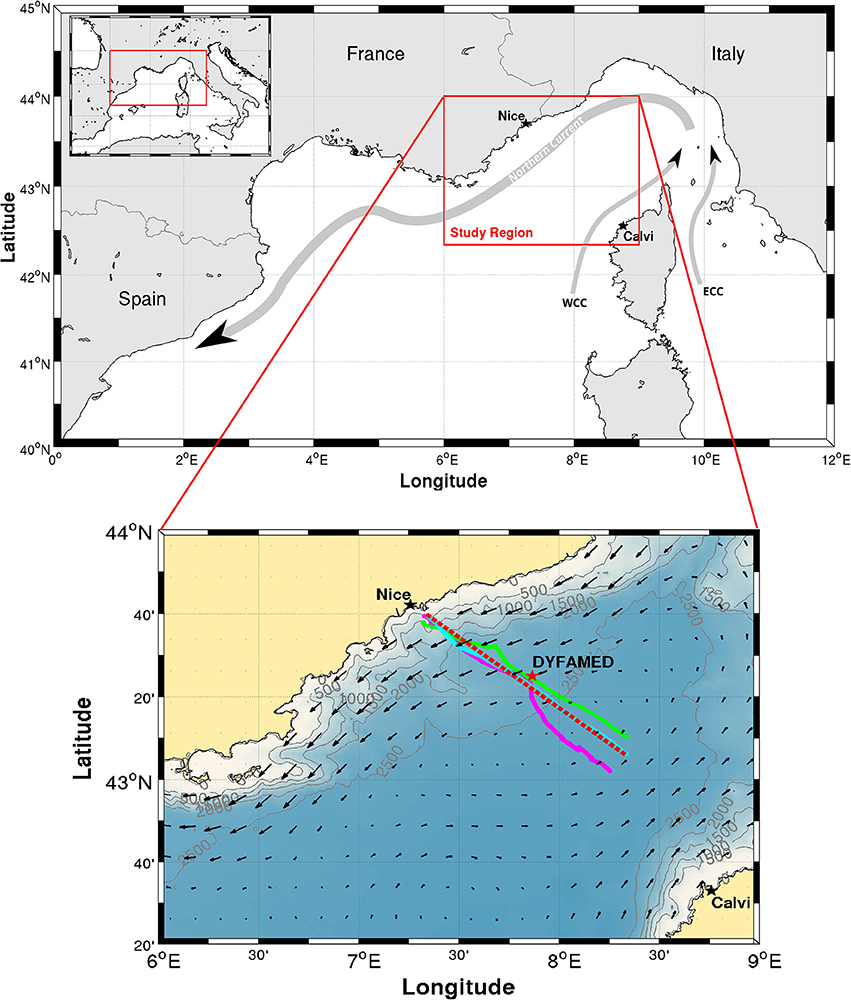
Figure 1. Map of the study area. Upper Northwestern Mediterranean Sea and a sketch of the Northern Current and the Western and Eastern Corsica Currents (WCC and ECC, respectively). Lower Zoom on the study region. Fall (28-31 October 2015), spring (29 April–3 May 2016) and summer (30 July–3 August 2016) glider tracks are plotted in Magenta, Green and Cyan, respectively. The red-dashed line is the ~100 km straight line between 43°40,000′ N, 7°19,842′ E (approximately the shelf break at the 500 m isobath) and 43°6,000′ N, 8°20,000′ E, on which glider casts are projected for Figures 6–8. DYFAMED oceanographic station is identified with a red star. Current arrows from Aviso altimetric product on 1 November 2016 are plotted for reference. The altimeter products were produced by Ssalto/Duacs and distributed by Aviso, with support from Cnes (http://www.aviso.altimetry.fr/duacs/).

This study focuses on the Nice-Calvi transect line (Figure 1, bottom panel). This line is regularly monitored as part of the Mediterranean Ocean Observing System for the Environment (MOOSE), a multi-scale and multi-site observation network targeting coastal/open ocean and ocean/atmosphere interactions. As part of MOOSE, monthly and annual ship-based observations are made along this transect. The transect is also regularly occupied by glider since 2007, with the aim of making it an endurance line. Located along the transect about 53 km offshore from Nice, the DYFAMED oceanographic station (red star on Figure 1) is also one of the most studied station of the basin (Marty et al., 2002). The good spatio-temporal coverage of the area makes it a perfect place for the first in situ application of the MiniFluo on the glider.

The annual cycle of the biogeochemical system functioning at DYFAMED may be described in three distinct periods: winter, spring and summer/fall (Avril, 2002; Migon et al., 2002). The winter period is dominated by deep convection and the water column is well mixed. It is followed by the spring bloom (March/April) occurring after the onset of stratification. The rest of the year, the NW Mediterranean exhibits a Deep Chlorophyll Maximum (DCM) at mean depth between 40 and 60 m that persists until being destroyed by the following winter convection (Lavigne et al., 2015). Maximum stratification is reached at the end of summer/early fall, and corresponds to a period when DOM accumulates in the surface waters (Jones et al., 2013). Smaller phytoplankton blooms may also occur in the fall.

2.2. MiniFluo Sensor

The sensor presented here is a new version of the MiniFluo, a field-portable fluorometer introduced by Tedetti et al. (2013), which is now glider-compatible. Basic working principles are recalled below.

2.2.1. Fluorescence Principle

Fluorescence is initiated when a fluorescent compound (or fluorophore) absorbs a photon at a specific wavelength. The fluorophore then moves from its electronic ground state to an excited state. Because the excited state is unstable, the molecule rapidly returns to the ground state by transmitting a photon of longer wavelength (i.e., of lower energy) than the excitation photon. Each fluorophore can be thus targeted by specific excitation (λ_Ex) and emission (λ_Em) wavelengths (with λ_Ex < λ_Em). Within a certain range, the intensity of the fluorescence light is proportional to the fluorophore concentration in the medium. Other fluorophores may however respond, with close or different magnitudes, to the same λ_Ex/λ_Em couple. The MiniFluo has two optical channels, enabling the simultaneous detection/quantification of 2 fluorophores of interest (one per optical channel). These channels (λ_Ex/λ_Em couples) are adjustable factory settings. For this study, we use data from a single MiniFluo on the glider, with the 2 channels centered on the λ_Ex/λ_Em 275/340 nm and 255/360 nm to preferentially target Trp-like and Phe-like fluorophores. Other compounds optically active in these spectral domains may potentially influence their fluorescence signals.

2.2.2. Optical and Mechanical Design

A sketch of the MiniFluo is presented in Figure 2. Each optical channel comprises one excitation section, one detection section, one monitoring section and one quartz right-angle prism (UV grade fused silica). The excitation section contains a deep UV LED emitting at λ_Ex. Photons emitted upward from the LED reach the right-angle prism and are redirected toward the sample for fluorophore excitation. The detection section, dedicated to the detection of fluorescence light emitted by excited fluorophores, incorporates a narrow band-pass filter centered at λ_Em, a quartz double-convex lens (UV grade fused silica), and a UV-enhanced silicon photodiode. A small fraction of emitted light from the LED is routed toward a second silicon photodiode (monitoring section), allowing the correction of any variation of the LED flux with time. This is because the measured fluorescence intensity is directly proportional to the intensity of the excitation light. The electronic and optical components of the MiniFluo are stored in a two-part housing (⊘ × L:75 × 60 mm) made of an anodized aluminum (upper part) and a copper cylinder (bottom part) (Figures 3a,b). The aluminum upper part incorporates a 4 mm quartz window (UV grade fused silica) fixed to the aluminum holding ring and a sealing joint. Four openings (2 per optical channel) necessary for the passage of light through the quartz window are made in the aluminum part. The housing holds a protective cover (removal optical cap, see Figures 2, 3c,d) made of black acrylonitrile butadiene styrene (ABS) thermoplastic polymer. This cap is fixed on the upper MiniFluo housing and protects the measurement system (photodiodes) from the ambient light. Openings at the front and the rear of the cap allow the water to flow underneath the cap and to be flushed out of the sampling volume by the glider motion (unpumped flow). The central part of the cap rests directly on the sensor window and separates the flow into the two sampling volumes (Figure 3c). Two quartz right-angle prisms embedded in this central part are responsible for the reflection of the excitation light toward the sampling volume. The housing fits to the scientific payload (dry compartment) of the SeaExplorer glider (Figures 3e,f).

FIGURE 2

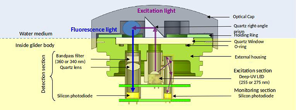
Figure 2. Technical sketch of the MiniFluo with the working principle of one of the two channels. The blue circle is the sample volume. The path of the excitation light (including the monitoring section with a thinner line) is drawn with purple arrows. The fluorescence light path is drawn with a blue arrow. The background color code highlight the wet (blue) and the dry (yellow) part of the sensor.

FIGURE 3

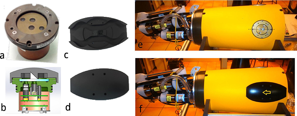
Figure 3. Glider-compatible MiniFluo. (a) Picture of the complete MiniFluo: anodized aluminum for the upper part and copper cylinder for the bottom part; (b) Diagram of the MiniFluo. Difference with Figure 2 is the electronic circuits placed underneath the photodiodes; (c) Optical cap with the quartz prisms placed at the center. The two channels for the through flow are also visible. (d) Optical cap (view from above); (e) MiniFluo installation on the SeaExplorer glider scientific payload; (f) MiniFluo installed with its optical cap.

2.2.3. Communication and Sampling Rate

The MiniFluo communicates with the SeaExplorer electronic payload board via an I2C (Master-Slave) protocol. The payload board being the master, it interrogates at regular intervals the three slave addresses of the MiniFluo (two temperature chips and the sensor's processor). Instructions from the glider to the MiniFluo include four main parameters, adjustable by the user via the SeaExplorer's payload configuration file. The first parameter is the measurements mode: LED ON (mode 1), LED OFF (mode 2) or LED ON-LED OFF (mode 3). The LED ON mode measures sample fluorescence taking into account the ambient light. The LED OFF mode measures the fluorescence resulting form ambient light only. The LED ON−LED OFF mode measures the sample fluorescence by removing the signal generated by the ambient light. The second parameter is the “caliber,” which selects the electrical capacitance of the integrator circuit after the photodiode and before the analog/digital (A/D) converter. Changes in the electrical capacitance are reflected into changes in the gain of the A/D converter, and thus in the range and sensitivity of the detection circuit (low capacitance = high sensitivity/low range and vice-versa). The caliber (C0–C7) can be adjusted from 3 to 86.5 μF, allowing changes in the sensitivity over a factor 28. The analog signal from the photodiode being digitized on 20 bits (1,048,576 counts), the range of the sensor can then be adjusted from 1 to 28 × 10⁶. The third parameter is the acquisition time (DACQ), expressed in ms. It corresponds to the time during which the LED is on and the photodiode collects the photons emitted by the compound. The higher the DACQ, the more the photodiode records fluorescence signal. For the mode LED ON−LED OFF, the measurement time is twice DACQ. The last parameter is the sampling interval (D2ACQ), which corresponds to the time (in ms) between two measurements, which determines the sampling frequency. For this study, the parameters used were: LED mode ON - OFF, caliber C0, DACQ = 600 ms and D2ACQ = 4,000 ms (about 0.2 Hz sampling frequency). Output from the MiniFluo to the glider includes raw fluorescence and monitoring values (raw binary counts) from both channels, as well as the emission/detection temperature values.

2.2.4. Calibration

The conversion from electronic counts (as returned by the sensor) to concentration data is performed in several steps. As described above, the MiniFluo is equipped with a compartment for monitoring excitation light in order to get rid of LEDs aging problems and to correct temperature effect on the LED power output. The concentration (C) of a certain compound is thus obtained by first converting raw count measurements (after de-spiking bad counts) to relative units (RU) that take the monitoring into account:

$\begin{array}{ll}{C}_{\text{RU}}=\frac{C_c-N_D}{C_m-N_D},& (1)\end{array}$

where C_c is the measured count value of the detection photodiode, C_m the measured count value of the monitoring photodiode and N_D = 4, 096 the constant electronic noise of the circuit (dark noise). The conversion from C_RU to physical units (ngL⁻¹ or μgL⁻¹) is done through a scale factor (SF) obtained from the calibration of each sensor (slope of the linear calibration curve):

$\begin{array}{ll}C=\frac{C_{\text{RU}}-B}{SF}.& (2)\end{array}$

Here B is the blank value, representing the sensor response in the absence of compounds of interest (intercept of the calibration curve).

The MiniFluo comes off-the-shelf with two laboratory calibrations (scale factors). The first calibration is similar to that described in Tedetti et al. (2013) and consists of measurements on standard solutions for the specific compounds targeted by the MiniFluo, in this case Trp and Phe. For each compound, N = 9 solutions with concentrations ranging from 0.1 to 10 μgL⁻¹ (C_i) were prepared from the dilution of pure standards (Phenanthrene Supelco 48569 and L-tryptophan Sigma-Aldrich ≃98%) into ultrapure Milli-Q water from Millipore system, final resistivity 18.2MΩcm⁻¹ at 25°C, pH~5. In order to avoid the preparation of large volume of standard solutions, the calibration was made by processing small amounts of solution transferred into quartz cuvette with optically polished bottom. These solutions were processed with the MiniFluo and the discrete C_RU were determined as the average relative unit values returned by the MiniFluo over about 1-min of measurements. The calibration procedure is illustrated in Figure 4. The scale factor SF, the intercept B_lab (laboratory blank) and their respective standard error were calculated using bootstrap (Efron and Gong, 1983) over 1,000 random replicates of the N calibration points (draw with replacements). For each replicate, the linear fit between C_RU and C_i was calculated on a least square sense. SF and B_lab are the average values of the slopes and intercepts of the replicates, while the standard error is their respective standard deviation (Equation 11 in Efron and Gong, 1983). Calibrations are reported in Table 1. Note that the large scale factor difference between MiniFluo #05 and #14 comes from a change in monitoring section materials between the two generations of sensor. This change has slightly modified the monitoring values, and thus SF via changes in C_RU values.

FIGURE 4

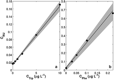
Figure 4. Examples of calibration curves for the MiniFluo#14. (a) Trp-like channel calibrated on standard solutions of Tryptophan. (b) Phe-like channel calibrated on water accommodated fraction (WAF) of Phenanthrenes (methylated and non-methylated). Black dots are the calibration points between prepared solutions (C_Trp or C_Phe) and relative units concentration measured by the MiniFluo (C_RU). Gray lines are the best fits calculated over the 1,000 random replicates of the calibration points. The shaded area represent the combined errors on scale factors and intercepts.

TABLE 1

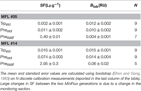
Table 1. Scale-factors (SF) and laboratory blank value (B_lab) for the compounds measured by the MiniFluo.

The second calibration targets only Phe and uses a water accommodated fraction (WAF) of crude oil. Oils/petroleum present in seawater contain a significant amount of methylated hydrocarbons (Wang et al., 1999; Guigue et al., 2011; Adhikari et al., 2015), which are generally more fluorescent than the non-methylated parent hydrocarbons (Ferretto et al., 2014). For the detection of hydrocarbons in seawater, a calibration conducted with the WAF (including methylated and non-methylated Phe) is thus more representative than a calibration based only on a standard of non-methylated Phe. The WAF is prepared by introducing 2 mL of crude oil (“Maya” type) at the surface of 1L of filtered seawater (filter pore size 0.2μm). The underlying water was then stirred with a magnetic stirrer for a minimum of 36 h. The water under the crude oil micro layer is considered the WAF. The calibration of the MiniFluo was accomplished by comparing C_RU output for several dilutions of WAF in seawater (25, 12.5, 6, 3, and 1.5%) with the “Phes” (methylated and non-methylated) concentrations determined by gas chromatography/mass spectrometry (GC/MS) according to Guigue et al. (2011, 2014). WAF scale factors were calculated by linear fitting in the range 0.0009 − 0.22μgL⁻¹ (information provided in sensor calibration sheet). Again, bootstrap was used to determine the error on SF and B_lab (see Table 1). This last calibration method (WAF) was used for Phe-like concentrations presented below.

2.3. Glider Measurements

Glider measurements presented here were performed during three campaigns across the NC and along the Nice-Calvi transect (Figure 1). The first campaign was realized by ALSEAMAR with one of their glider (code name SEA007) while the two other campaigns were carried out with the Mediterranean Institute of Oceanography's SeaExplorer glider (code name SEA003). The fall campaign was conducted between 28 October and 10 November 2015, the spring campaign between 29 April and 20 May 2016 and the summer campaign between 25 July and 4 August 2016. For the three campaigns, the glider was equipped with a pumped conductivity-temperature-depth sensor (Seabird's GPCTD) from which the conservative temperature (Θ), the absolute salinity (S_A) and the density anomaly referenced to the surface (σ₀) are derived using TEOS-10 toolbox (McDougall and Barker, 2011). This GPCTD is also equipped with a dissolved oxygen (O₂) sensor (Seabird's SBE-43F) from which concentrations are derived. A WetLabs ECO FLBBCD was also mounted on the glider for measurements of Chlorophyll-a (Chl-a) fluorescence (λ_Ex/λ_Em: 470/695 nm), backscattering at 700 nm (BB700) and humic-like fluorophore fluorescence (λ_Ex/λ_Em: 370/460 nm) expressed in μgL⁻¹ equivalent quinine sulfate units (μgL⁻¹QSU). For this sensor, the manufacturer's calibration was used. This means that Chl-a concentrations were not calibrated on in situ measurements and are rather expressed in their equivalent of Thalassiosira weissflogii phytoplankton mono-culture. Measured Chl-a concentrations values were also shifted by an offset in order to obtain [Chl-a]=0 at 250 m (e.g., Lavigne et al., 2015). This was achieved by subtracting 0.02μgL⁻¹ (fall campaign) and 0.08μgL⁻¹ (spring and summer campaigns) from the whole dataset. In a complement to these relatively common glider measurements, the MiniFluo was used on an exploratory basis: never before such high frequency measurements of Trp and Phe were performed from a glider.

Only subsets of the glider campaigns are presented here (see Figure 1 caption for dates). They consist of about the first 100 km of the Nice-Calvi transect (red-dashed line in Figure 1), with the DYFAMED station located at x = 53.2 km. This section was chosen because of the relatively good overlap of the glider tracks during the three surveys. Note that while the glider traveled from Nice toward Calvi for the fall and spring transects, the summer transect was realized in the opposite direction. Glider observations were first processed with the Socib glider toolbox (Troupin et al., 2015) for cast identification and georeferencing. Then, in order to directly compare the three surveys, each cast was projected to its closest point on the straight dashed-line of Figure 1. Each transect is displayed in term of its distance from the origin of the transect (Figures 6–8). The horizontal resolution between these transects is variable since the depth of glider dives was different from one deployment to the other, respectively 300, 650, and 400 m. In order to focus on biogeochemical variables, only the top 250 m are considered here, a depth range where most of the variability is found.

3. Results

3.1. MiniFluo In situ Working Principle

This section recalls useful observations made during the early glider deployments with the MiniFluo. These have revealed some limitations and interesting observations regarding the sensor's in situ working principle.

3.1.1. Environmental Blank Value

One limitation when using the sensor on the glider is the need to adjust the blank B from its laboratory value (B_lab) to an environment-specific value (B_env). Reasons for this are two-fold. First, different background fluorescence levels (fluorescence for concentration equal to zero) may be found between natural environment and ultrapure water used in laboratory. Second, it is worth noting that the error on the blank for WAF calibrations is on the same order of magnitude than the value itself. This shows the sensitivity of the parameter B during the calibration process. The use of laboratory blanks in natural environment would lead to a shift in measured concentrations (e.g., negative concentration or impossibility to reach concentration equals zero) that it is possible to avoid. In order to account for this difference, our strategy is to replace the laboratory blank value (B_lab) from the calibration sheet by a user-defined value specific to the studied environment. In this study, B_env values have thus been chosen as the minimum relative-unit of the de-spiked dataset, so that the minimum measured concentration of a certain compound far from dynamical biogeochemical region converges toward zero. Table 2 summarizes the different values used for this study.

TABLE 2

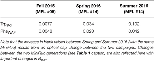
Table 2. Environment-specific blank values, B_env(RU), for the different glider campaigns.

3.1.2. Optical Cap

As shown in Figures 2, 3, the MiniFluo is equipped with a removable optical cap located outside the glider body. This cap contains quartz prisms and is an essential optical component of the sensor. The choice of material and inner finish of the cap is thus important since the latter must be opaque to ambient light. This is because even with the LED ON—LED OFF mode, ambient light can still contaminate the fluorescence signal entering into the detection section. This problem was revealed during a deployment made with an early version of the cap designed by 3D Selective Laser Sintering with a polyurethane resin. The deployment using this cap shows that measurements over the top ~5 m (but mostly limited to the 0–2 m range) are contaminated by ambient light during daytime (Figure 5a). The new version of the cap, made of black ABS polymer, now better protects the optical chamber from ambient light, since no systematic departure from the mean is observed for measurements near the surface in the 0–5 m depth range (Figure 5b). In addition to this new material, laboratory experiments revealed that a resin siloxane paint treatment reduces internal reflection/scattering of light and/or possible fluorescence of ABS material inside the optical chamber, which in turn reduces the noise level and improve the detection limit of the sensor (results not shown).

FIGURE 5

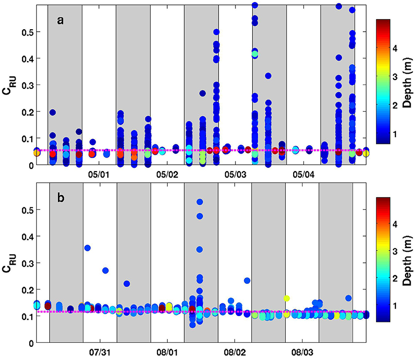
Figure 5. Timeseries (5 days) of the relative units concentration (C_RU) for one MiniFluo channel (Trp-like) along the Nice-Calvi transect using the same MiniFluo with different optical caps. (a) Data from the second glider mission (1–5 May 2016) using the original optical cap. (b) Data from the third glider mission (31 July to 4 August 2016) using the new version of the cap. Only measurements in the 0–5 m depth range are plotted and each discrete measurement is colored according to its depth (see colorbar). The vertical gray bands correspond to the 6:00–18:00 range, i.e., the approximate daylight period. The dashed-magenta line is the mean value for this depth range.

Aluminized coating is used on the rear face of prisms to allow a maximum reflection in the UV range. Since the prisms inside the optical cap are in contact with seawater, a light blocking sealing tape (Thermo Scientific) is applied on their base to protect from corrosion. Some prisms used without this special care have shown traces of corrosion of their surface. For additional precaution, the cap and prisms are removed after each glider deployment, carefully rinsed in ultrapure milliQ water and stored in a dry place.

3.1.3. Effect of Temperature on Fluorescence Measurements

Temperature impacts in situ fluorescence measurements in two ways. First, temperature influences LED power output of the sensor (excitation light), which in turns modifies the fluorescence intensity (emission light). As mentioned above, the MiniFluo is equipped with a monitoring section which is used to correct this effect. Second, it is well established that DOM fluorescence intensity is influenced by the temperature of the sample (FDOM thermal quenching). Recent developments in the field of sensor-derived fluorescence suggest a decrease of humic-like (Watras et al., 2011; Downing et al., 2012; Ryder et al., 2012; Yamashita et al., 2015) or Trp-like (Khamis et al., 2015) fluorescence intensity on the order of [0.6–1.5]% per °C increase in temperature. Temperature tests were performed with the MiniFluo over the range 7–33°C using a thermostated chamber. Results (not shown) are in accordance with these observations. Given the temperature range considered here (roughly 13-17°C, Figure 9), we did not apply any temperature correction on fluorescence data.

3.2. Observations

Figures 6–8 show contour plots of the glider data from the three deployments, respectively fall 2015, spring 2016 and summer 2016, along the first 100 km of the Nice-Calvi transect and for the depth range 10–250 m. As it is shown below, the maximum offshore extent of the NC during these 3 transects (e.g., in Figure 6) is about 60 km from the coast, further than the DYFAMED station. In order to obtain data representative of the “offshore” region, i.e., a portion of the transect not under the direct influence of the Northern Current, we used the dashed box drawn in Figures 6–8 (70–80 km from the shelf break). Average profiles over this region are presented in Figure 9, which summarizes the seasonal differences for every variables presented in these contourplots. Physical and biogeochemical features are presented below.

FIGURE 6

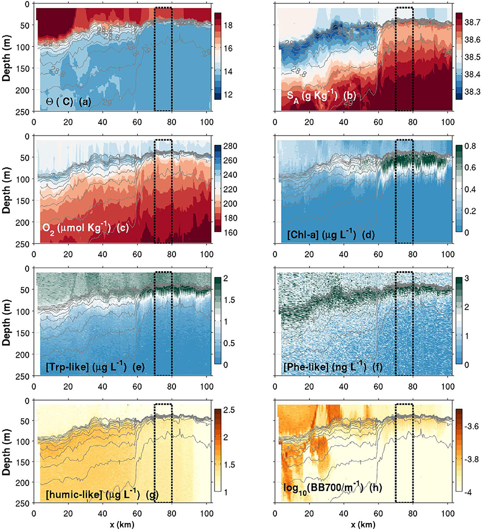
Figure 6. Contours plots of various variables measured by the glider in function of depth and along-transect distance (x) for the fall transect. (a) Conservative temperature; (b) Absolute salinity; (c) Dissolved oxygen concentration; (d) Chlorophyll-a concentration; (e) Tryptophan-like concentration; (f) Phenanthrene-like concentration; (g) Humic-like concentration; (h) Turbidity measured as the backscattering signal at 700 nm. Isopycnals are plotted in each panel with thin solid light gray lines (values identified in a,b). The top 10-m of the water column have been discarded according to Figure 5 data. The black dashed box corresponds to region from which averaged seasonal profiles have been calculated (plots in Figure 9).

3.2.1. Physical Features

Θ and S_A transects are presented in Figures 6–8a,b. Thin gray lines in theses figures are the isopycnals (σ₀). Comparison of the isopycnal slopes (representative of the geostrophic currents) between fall, spring and summer observations suggests that the Northern Current is wider and weaker during the fall (isopycnals tilted in the ~0–60 km range, Figure 6), compared to the spring (~0–40 km, Figure 7) and to the summer (~0–30 km, Figure 8) where the isopycnal slope is more pronounced. The fall transect however exhibits a sharp front at the offshore limit of the Northern Current (~60 km) where, for example, the isopycnal 29 kg m⁻³ moves vertically by more than 100 m over less than 10 km.

FIGURE 7

Figure 7. Same as Figure 6, but for a spring transect. Note that the colorbar of the Chl-a has been changed compared to Figure 6.

FIGURE 8

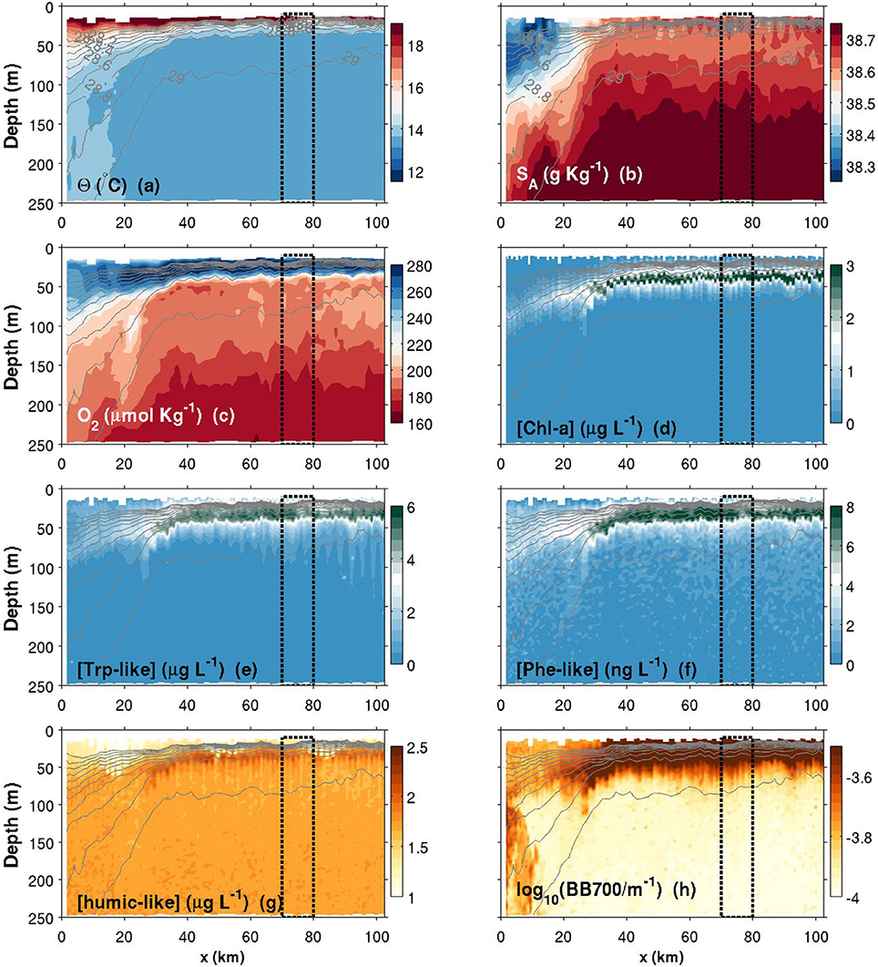
Figure 8. Same as Figure 6, but for a summer transect. Note that the colorbars of Chl-a, Trp and Phe have been changed compared to Figure 6.

To better highlight stratification differences between the seasons, the buoyancy frequency squared, $N^2=-\frac{g}{{\rho }_0}\frac{\partial {\sigma }_0}{\partial z}$, is plotted in Figure 9i. Here ${\rho }_0=1,030\text{kg}{\text{m}}^{-3}$, is a constant reference density and g = 9.81m²s⁻¹ the gravitational acceleration. The depth of the pycnocline may be defined as the peak in N² and is generally considered as a physical interface affecting biogeochemical dynamics. In the offshore region, the pycnocline is centered at a depth of 46, 14, and 39 m, respectively for the spring, summer and fall. The base of the pycnocline, a depth range where most biogeochemical tracers exhibits departure from their deep and nearly constant background values (Figure 9), is located at 53, 38, and 51 m, respectively for the three seasons. It is defined, after visual inspection of N² profiles, as the depth where N² > 8 × 10⁻⁵s⁻² (see Figure 9i).

FIGURE 9

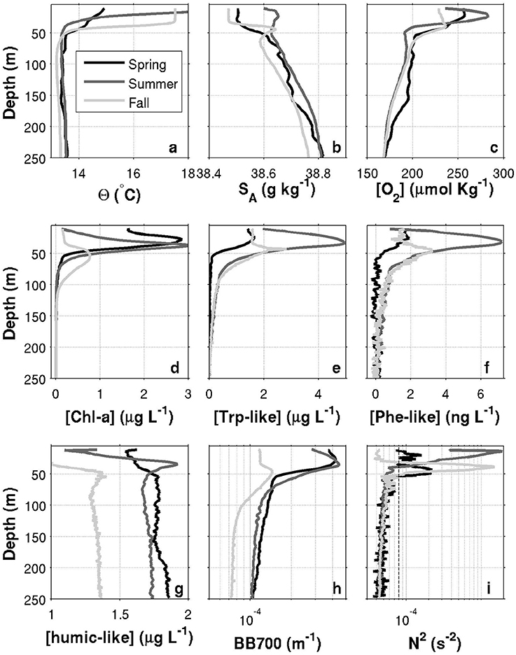
Figure 9. Seasonal profiles in the offshore region of the Nice-Calvi transect (offshore from the influence of the Northern Current). Each panel shows the average profiles over the 70–80 km range of the transect (dashed box in Figure 6). (a) Conservative temperature; (b) Absolute salinity; (c) Dissolved oxygen concentration; (d) Chlorophyll-a concentration; (e) Tryptophan-like concentration; (f) Phenanthrene-like concentration; (g) Humic-like concentration; (h) Turbidity measured as the backscattering signal at 700 nm; (i) Buoyancy frequency squared (variable not presented in Figure 6). The vertical dashed line corresponds to N² = 8 × 10⁻⁵ s⁻², a threshold used to calculate the base of the pycnocline. One profile for each of the three glider deployments is presented, respectively for fall 2015 (light gray), spring 2016 (black) and summer 2016 (dark gray). Note that while spring and summer data are from 2016, fall data are from 2015.

Near the coast, surface waters are generally warmer and fresher for all seasons, with the exception of a near-coast warmer but saltier layer during the fall (Figures 6a,b, top ~100 m, 0–20 km). For the same season, an interesting feature is the presence, within the Northern Current, of a 50–60 m thick subsurface lower-salinity layer (Figure 6b). Although this layer was reported in previous studies (e.g., Andersen et al., 2009; Piterbarg et al., 2014), dynamical reasons for its existence are however unknown at this stage. In summer, a relatively large salinity inversion is also visible in the offshore region as shown in Figure 9b (light gray, ~25–75 m).

3.2.2. Biogeochemical Features

The depth of the pycnocline generally delimits relatively well oxygenated surface waters ($\left[O_2\right]>250\text{μmolk}{\text{g}}^{-1}$) from deeper waters where a vertical gradient is found down to roughly $\left[O_2\right]~170\text{μmolk}{\text{g}}^{-1}$ at 250 m (Figures 6–8c, 9c). The spring O₂ profile however shows a deviation from the two other profiles at depth between roughly 75–200 m. This O₂ increase at depth also corresponds to a decrease in S_A (Figure 9b) and is visible as a sub-surface maximum/minimum on the contourplots (see Figures 7b,c). The origin of this submesoscale-size feature (~10 km in the along transect direction) is unknown.

The spring campaign was realized after the phytoplankton bloom since the DCM was already formed (Figure 9d). Chl-a concentrations during spring and summer are more than three times those of the fall survey, with a maximum value in the summer. The depth of the DCM also increases throughout the year (minimum in spring and maximum in the fall). While its depth matches the depth of the pycnocline in summer, the DCM is shallower than the pycnocline in spring and deeper in fall. It is important to recall that Chl-a concentrations were not calibrated against in situ phytoplankton collection. Concentrations reported here are also slightly above the climatological values reported in literature (e.g., Lavigne et al., 2015).

Humic-like and Backscattering measurements (Figures 6, 9g,h) are presented as they are standard measurements on gliders. However, although meaningful for understanding biogeochemical dynamics in the NW Mediterranean, their extensive analysis is beyond the scope of this study. Only observations relevant for the discussion made in Section 4 are presented. The fall campaign was realized after important rain events. This campaign is marked by more turbid water (high backscattering) close to the shore (Figures 6h, 9h), with the exception of the subsurface lower salinity layer discussed above (Figures 6b, 9b), which is associated with relatively “clear” (low backscattering) water. Offshore, the depth of the DCM matches the depth of maximum backscattering relatively well for all three seasons. However, the depth of the DCM only matches humic-like peak during the summer and fall. In spring, the slight decrease in humic-like in the 75–200 m range corresponds to the submesoscale feature observed in previous subsection (decrease in S_A and increase in O₂).

Comparison between Chl-a and Trp-like measurements (Figures 9d,e) suggests that both tracers do not have the same seasonal dynamics. For example, while Chl-a concentrations are relatively stable between spring and summer, Trp-like concentrations are multiplied approximately by a factor 3. Moreover, while Chl-a concentrations are divided by 3 between the spring and the fall, Trp-like concentrations are higher during the fall. Also, the vertical position of Trp-like peaks is always shallower than the peaks in Chl-a. This difference is 4 m during the spring and summer, and 10 m in the fall (see Table 3). The latter peak in Trp-like fluorescence is also sharper than during the spring or summer periods. In summer and fall, the DCM matches relatively well the position of the base of the pycnocline, while in spring it is much more shallower (Table 3).

TABLE 3

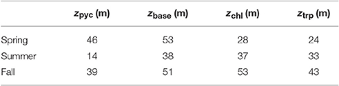
Table 3. Position of maximum subsurface Chl-a (z_chl) and Trp-like (z_trp) concentrations in relation to the position of the center of the pycnocline (z_pyc) and its base (z_base).

While the Phe-like concentrations mimic relatively well those of Trp-like in the offshore region for all seasons (Figure 9), their dynamics are contrasted during the fall in the near-shore region. Indeed, Phe-like concentrations are relatively high near the coast while the Trp-like ones are rather low (Figures 6e,f). The relative continuity of Phe-like concentration throughout the front in Figure 6f suggests an accumulation of this PAH just below the pycnocline, with about the same concentration in coastal and offshore waters. This behavior is quite different from the other biogeochemical tracers that mostly exhibit striking differences between both sides of the front.

4. Discussion

4.1. Confidence in MiniFluo Measurements

One limitation to our study is the relative absence of hindsight with the MiniFluo technology. For example, fine tuning improvements were made between the different campaigns presented here (e.g., monitoring section change between MiniFluo #05 and #14 and optical cap change between spring and summer 2016 missions). Although the scale factor and blank values were adjusted between these missions, the repetition of the measurements with a single setup over many years would help identifying if one part of the signal is due to instrumental changes. While the relative coherence in concentration range observed from one campaign to the other is reassuring, discrete water samples at the time of glider deployment and/or recovery would certainly increase our confidence in the measurements. Bootstrap analysis on scale factors suggests a maximum error on measurement of 7% for the Trp and 10% for the Phe (WAF calibration) with MiniFluo#14, and respectively 50 and 33% with MiniFluo#05. It is likely that the change of monitoring section between the two MiniFluo generation has led to a decrease in the calibration error.

Trp-like fluorophore concentrations measured with the MiniFluo in the present work (0–6 μgL⁻¹) are higher than concentrations of total (free + combined) dissolved Tryptophan determined by alkaline hydrolysis and HPLC in coastal marine waters (0.2–0.4 μgL⁻¹; derived from Yamashita and Tanoue, 2003) but close to those observed in freshwaters (2–8.5 μgL⁻¹; derived from Wu and Tanoue, 2001). Two assumptions can be made to explain why the MiniFluo provides higher concentrations. First, while HPLC analyses allow the determination of dissolved Trp concentrations only, the MiniFluo also record fluorescence due to Trp bounded to particulate matter that may lead to an increase in the total Trp-like fluorescence signal in seawater. Second, as highlighted by Carstea et al. (2016), other organic compounds, such as lignins, may also fluoresce in the Trp spectral domain. Discrete molecular analyses of dissolved tryptophan combined with MiniFluo measurements would help understanding the real contribution of dissolved tryptophan compound in the MiniFluo-derived Trp-like fluorescence. Interestingly, Khamis et al. (2015) found Trp-like fluorophore concentrations in groundwater ranging from 3 to 15 μgL⁻¹, i.e., very close to the concentration found here, using UviLux (Chelsea ctg) and Cyclops 7 (Turner Designs) fluorometers.

Phe-like fluorophore concentrations measured here with the MiniFluo (0–8 ngL⁻¹) are derived from calibrations taking into consideration non-methylated and methylated Phe (WAF solutions). These are in the same range than the concentrations of dissolved Phe (non-methylated + methylated) determined by GC-MS in the open Mediterranean Sea (0.4–4 ngL⁻¹; Berrojalbiz et al., 2011) and in the coastal Mediterranean Sea (i.e., Bay of Marseille, 5–50 ngL⁻¹; Guigue et al., 2011, 2014).

It should be noted that our fluorescence measurements were not corrected for inner filtering effects, because absorption measurements were not conducted during our glider cruises. In these waters (Nice-Calvi transect, within the 0–200 m layer), DOM absorption measurements performed with a multiple path length, liquid core wave-guide UltraPath, revealed maximal absorption coefficients at 280 nm of 0.8 m⁻¹ at the seasonal level (Organelli et al., 2014). Assuming an exponential fit for absorption spectra and a high spectral slope of 0.050 nm⁻¹ over the range 280-250 nm, maximal absorption coefficients at 250 nm would be of 3.6 nm⁻¹. Therefore, since DOM absorption coefficients at the two excitation wavelengths of the MiniFluo (255 and 275 nm) remain <10m⁻¹ in this marine area, we can reasonably assume that inner filtering effects had no significant influence on our fluorescence data (Stedmon and Bro, 2008).

It is also important to note that concentrations reported here were derived from laboratory calibrations. The relatively good agreement with historical data suggests that these calibrations are sufficient to capture the bulk part of the targeted signal. However, as it is commonly done for Chlorophyll fluorescence measurements, in situ calibration on water samples would be essential to refine estimates and assess concentrations with greater confidence.

4.2. Physical-Biogeochemical Interactions across the Northern Current

The general understanding of the NC dynamics is that it is deeper, stronger and closer to the coast during the winter, with a relative slowing down throughout the year, becoming widest and shallowest in the early fall (Millot and Taupier-Letage, 2005; Birol et al., 2010; Declerck et al., 2016). Results presented here rather suggest no significant difference in isopycnal positioning in the NC between the spring and summer, but a wider and shallower current during the fall. It is important to note that above the seasonal variability of the NC, the mesoscale activity (e.g., meanders) may also change the positioning of the NC on much shorter timescales (Millot, 1991; Flexas, 2004), making a generalization of our snapshot transects hazardous. One important aspect to note, however, is that the offshore influence of the NC may reach further than the DYFAMED station (see for example the position of the front at x≃65 km in Figure 6). This observation shows that DYFAMED is not free from the influence of the NC as it was suggested in the past (Andersen and Prieur, 2000; Marty et al., 2002).

The mesoscale activity plays an important role for the physical-biogeochemical coupling in the NW Mediterranean, since the NC acts as a physical barrier between coastal and offshore waters (André et al., 2009; Barrier et al., 2016; Ross et al., 2016). A recent study by Piterbarg et al. (2014) suggests that the use of ocean gliders is a promising tool to address the role of mesoscale activity of such a frontal system. The clear distinction of the different zones (coastal, front, offshore) visible in Figures 6–8 confirms this potential. The relative good match between the regional Aviso altimetry product used to draw current arrows in Figure 1 is also worth noting since remote sensing is a powerful tool to address mesoscale dynamics of such current systems (e.g., Birol et al., 2010). Here, the surface expression of the NC main vein seems to disappear just offshore from DYFAMED (Figure 1) consistent with position of the NC in the glider transect (frontal zone located just offshore from DYFAMED in Figure 6). Although mesoscale interactions are beyond the scope of this study, it is worth recalling that the new physical-biogeochemical data presented here may help addressing the question. One interesting feature revealed by the MiniFluo is the difference between Trp-like and Phe-like behavior across the front. While Trp-like fluorophore exhibits a clear transition at the front (Figure 6e), Phe-like fluorophore displays a relative continuity throughout the frontal zone (Figure 6f). This intriguing difference will be further discussed below.

An important and still open question concerns the mechanisms (likely submesoscale interactions) driving the horizontal and vertical exchanges at the frontal zone. The first glider measurements of physical-biogeochemical interactions across this frontal zone was presented by Niewiadomska et al. (2008) during the winter time, i.e., when NC velocities are higher and the mesoscale activity at its maximum. Their study was carried out along the first half of the transect presented here and highlighted the importance of biogeochemical tracers for understanding submesoscale frontal dynamics. Among other things, they revealed the presence of what looks like downwelling at the front edge. Such vertical re-distribution of biogeochemical tracers at the front edge is likely to trigger photosynthesis production if nutrients are brought to the euphotic zone. In our data, spring contourplots (Figure 7) may suggest some similar downwelling at the front edge. What resembles a downwelling patch is located approximately at the same position (~25–40 km), but less pronounced in terms of depth, compared to the study of Niewiadomska et al. (2008) (see S_A and O₂ inversions in the 50–150 m depth range, and the deepening of Chl-a, Trp-like, Phe-like and BB700 data).

Another interesting submesoscale feature is the subsurface low-salinity/high-oxygen anomaly found between 100–200 m during the spring campaign (see Figures 7b,c near x = 80 km). This structure, which has also a signature in the humic-like plot (Figure 7g), is associated with a local “doming” of the isopycnals that suggests a subsurface eddy. Recent observations of submesoscale coherent vortices (SCV) that resembles the structure observed here were reported for the same geographical area (Bosse et al., 2015, 2016). However, their origins are likely different since SCV reported in these studies are observed deeper (200–500 m) and are associated with high-salinity anomalies. Nevertheless, the new structure revealed here is worth exploring in existing datasets since its physical-biochemical signature suggests a key role in lateral exchanges of biochemical tracers. Again, glider biogeochemical observations, including the one with the MiniFluo, may give useful insights on the origin and the fate of such small-scale processes.

4.3. Tryptophan-Like Fluorophore Dynamics

Previous observations of Trp-like fluorescence in marine environment (not under strong anthropogenic pressure) suggest that it is particularly high in region of maximum primary productivity (Stedmon and Markager, 2005). The high vertical resolution of the present dataset rather suggests that this relationship may be more complex. For example, mean profiles show that the maximum Trp-like fluorescence is always shallower than the maximum Chl-a fluorescence (Table 3). This difference may be due to the vertical mismatch between Chl-a fluorescence and biomass, or to the vertical distribution of planktonic communities. Unfortunately, no plankton measurements are available to test these hypotheses.

The seasonal dynamics also suggests that Trp-like concentration is not simply proportional to the primary productivity: while both tracers peak in the summer, their dynamics for spring (high Chl-a/low Trp) and fall (high Trp/low Chl-a) are contrasted (see Section 3.2.2). Three hypotheses are provided to explain the seasonal decoupling between Trp and Chl-a concentrations. First, it may suggest that a specific group of microalgae may be responsible for the Trp production (Romera-Castillo et al., 2010). In the studied area, the succession of phytoplankton species during transition from a mesotrophic production regime to an oligotrophic production regime is well described (Andersen and Prieur, 2000; Marty et al., 2002). The diatom bloom that develops in March is followed by a predominance of small-size phytoplankton species (Chromophyte nanoflagellates and picoplankton). Re-increase of diatom biomass during the fall may be observed due to wind events that re-inject nutrients in the productive layer. Thus, in the summer period, when we observed the maximum Trp-like fluorescence, small size nano- and pico- plankton predominated over the phytoplankton community, whereas microphytoplankton is at its lower contribution (Ramondenc et al., 2016).

The second hypothesis involves changes in bacterial activity following the spring bloom. Trp releases in the medium have already been attributed to bacterial degradation of DOM by marine microbes (Stedmon and Cory, 2014). In this scenario, the increase in bacterial degradation of phytoplankton-derived DOM after the spring bloom is followed by an increase of the Trp pool in the surface/sub-surface waters. This hypothesis is however questionable since measurements realized after the spring bloom show relatively low Trp-like concentrations.

The third hypothesis is related to preservation/refractorization processes of DOM that could lead to an accumulation of Trp in Mediterranean surface waters. DOM accumulation during summer oligotrophy has already been observed in the surface water in NW Mediterranean (Avril, 2002; Goutx et al., 2009; Xing et al., 2014). Interestingly, the co-accumulation in the summer of other DOM descriptors (e.g., humic-like and Phe-like fluorophores) suggests that preservation/refractorization processes are predominant over degradation processes at this time of the year. Both abiotic and biotic processes may account for such preservation. On one hand, refractorization of labile DOM, of which the tryptophan may be a proxy, is triggered under UV irradiation in the surface water column (Mopper et al., 2015), subtracting refractorized DOM from the bacterial attack. On the other hand, a reduced utilization of labile compounds by nutrient-limited bacteria during oligotrophic summer conditions (Thingstad et al., 1997) may also lead to such Trp-like accumulation.

It is however very likely that the distribution of Trp reflects the integration of these three processes. The accumulation of DOM in surface Mediterranean oligotrophic waters in summer is an important driver for the efficiency of carbon and nitrogen export to the deep ocean. In the NW Mediterranean, this pattern has however mostly been assessed using variations in bulk DOC and DOM (Avril, 2002; Pujo-Pay and Conan, 2003; Santinelli, 2015). Only few studies have addressed the dynamics of DOC components (Bourguet et al., 2009; Goutx et al., 2009; Organelli et al., 2014; Xing et al., 2014), and the relative importance of diagenetic processes (microbial production, microbial degradation and phototransformation) responsible for production and removal of the DOM pool remains difficult to discern. Interestingly, Trp-like fluorescence presented here provides the first high frequency measurements of nitrogenous dissolved material (DON) component, showing this accumulation in summer. In oligotrophic regions, the DON material plays a particularly vital role in oceanic biogeochemical cycles.

The measurements of Trp-like fluorophore variations reinforce the idea that FDOM may be a good proxy for processes influencing the wider DOM pool. In the present study, the relative localization of Trp-like fluorophores along Chl-a depth profile and the temporal decoupling between Trp and Chl-a accumulation suggest that the Trp-like fluorescence is not only a marker of primary production but could also give more subtle information on the microbial processes occurring.

4.4. Phenanthrene-Like Fluorophore Dynamics

Ocean surface deposition of atmospheric PAHs is now being recognized as a major source of carbon in the ocean (González-Gaya et al., 2016). Their role in DOM dynamics and carbon export is however uncertain. New high resolution measurements using glider and optical sensors such as the one presented here may help addressing this question.

One of the most extensive study reporting PAHs concentrations in Mediterranean waters (Berrojalbiz et al., 2011) confirms that Phe and its alkylated (methylated) homologs were the predominant PAHs in water samples (dissolved and particulate) and in plankton biomass. However, most of the water samples used in this study were taken from the surface, where concentrations are rather low compare to the sub-surface. For the few samples taken at the DCM, these authors found that dissolved PAH concentrations were systematically higher than in surface waters. The high vertical resolution of the observations presented here confirms this pattern, which suggests an accumulation of Phe-like material just below the pycnocline at all seasons (Figure 9f). In the light of these new results, a re-interpretation of physical and biogeochemical processes affecting PAH concentrations in surface waters and in plankton (Berrojalbiz et al., 2011, e.g., schematics presented in their Figure 5) can be considered.

The good spatial coverage possible with glider-based observations also reveals other interesting features such as the Phe-like fluorescence continuum observed throughout the frontal zone during the fall (Figure 6f), while all other physical and biogeochemical tracers show striking differences on both sides of the front. Such intriguing results are certainly worth investigation. Among other questions to answer, it would be interesting to decipher whether Phe-like fluorescence observed here is related to direct atmospheric input, or rather land drainage origin. The relative abundance of Phe and methylated Phe may be used to distinguish the origin (petrogenic vs. pyrogenic) of these compounds (Prahl and Carpenter, 1983; Garrigues et al., 1995). In general, the predominance of Phe among its methylated homologs reflects a pyrogenic origin (i.e., combustion products routed by atmospheric aerosols for instance). On the other hand, high methylated Phe/Phe ratios are attributed to a petrogenic origin (i.e., crude oil derived from sea-based activities). The combination of glider measurements with traditional water sample collection would thus shed some light on Phe dynamics in the NW Mediterranean Sea.

5. Conclusion and Perspectives

Glider-based measurements with the MiniFluo have revealed some insights about DOM dynamics in the Mediterranean Sea that have never been observed before. Whether from natural (Trp-like) or anthropogenic (Phe-like) origin, the spatio-temporal distributions of the targeted fluorophores have raised questions that will need to be addressed in the future. Some hypotheses were formulated to explain both the temporal and spatial miss-match between Chl-a and Trp and the origin of Phe-like PAH observed just below the pycnocline at all seasons. Among the following years, repetitions of the transect occupied for this study with the glider and the MiniFluo may answer part of this questioning.

The oceanic DOM pool is a key component of the global carbon cycle. Over the recent years, it has been receiving increased attention as its role on atmospheric carbon sequestration is becoming clearer. While traditional measurements including water samples collection will always be needed, new observation strategies involving unmanned vehicles and optical sensors may be a key step toward our understanding of DOM dynamics and the biological pump. Glider-based MiniFluo measurements presented here support the promising contribution of this strategy in the future.

In complement to the measurements presented here, the addition to the glider payload of another (or more) MiniFluo targeting different fluorophores would be interesting. The goal here is to reconstruct elements of the excitation-emission fluorescence matrix that it is possible to obtain in laboratory by fluorescence spectroscopy. Simultaneous measurements of several DOM fluorophores will further increase our understanding of DOM dynamics (composition, origin, fate, etc.). For example, our group already owns another MiniFluo targeting two other PAHs: Fluorene-like (λ_Ex/λ_Em: 260/315 nm) and Pyrene-like (λ_Ex/λ_Em: 270/376 nm). The specific combination of this other MiniFluo with the one presented here would be an ideal tool for oil spill detection and risk assessment. Other λ_Ex/λ_Em couples may also be considered to target other natural DOM in the environment.

Author Contributions

MG, MT, and LB initiated the development of the MiniFluo and its inclusion on the SeaExplorer glider. FC led the study, including the data processing and the writing, in close relationship with MG and MT. All other authors contributed to the writing, FB specially for the technical aspect about the MiniFluo and AP and AD for the physical oceanographic environment of the study area.

Funding

This study is a contribution to the European project NeXOS–Next generation Low-Cost Multifunctional Web Enabled Ocean Sensor Systems Empowering Marine, Maritime and Fisheries Management, is funded by the European Commission's 7th Framework Programme—Grant Agreement N°614102.

Conflict of Interest Statement

The authors declare that the affiliation of FB and LB, the manufacturer of the MiniFluo and the glider SeaExplorer, do not preclude to the scientific independence of this scientific work which meets the standard of academic research.

All other authors declare that the research was conducted in the absence of any commercial or financial relationships that could be construed as a potential conflict of interest.

Acknowledgments

The authors would like to thanks ALSEAMAR, the Laboratoire d'Océanographie de Villefranche-sur-mer, the SAM service at MIO and the Antedon crew who made the three glider deployments possible. Several other contributors who have participated to the development of the sensors, mostly via internships or laboratory work, are listed here in a alphabetical order: C. Bachet, C. Guigue, C. Germain, P. Joffre, and G. Wassouf. FC personally thanks the entire SeaExplorer team at ALSEAMAR for their support during the field campaigns, including the precious time spent discussing glider technology and piloting strategies. The authors finally thank two reviewers for their helpful comments.

References

Adhikari, P. L., Maiti, K., and Overton, E. B. (2015). Vertical fluxes of polycyclic aromatic hydrocarbons in the northern Gulf of Mexico. Mar. Chem. 168, 60–68. doi: 10.1016/j.marchem.2014.11.001

CrossRef Full Text | Google Scholar

Amin, S. A., Hmelo, L. R., van Tol, H. M., Durham, B. P., Carlson, L. T., Heal, K. R., et al. (2015). Interaction and signalling between a cosmopolitan phytoplankton and associated bacteria. Nature 522, 98–101. doi: 10.1038/nature14488

PubMed Abstract | CrossRef Full Text | Google Scholar

Andersen, V., Goutx, M., Prieur, L., and Dolan, J. R. (2009). Short-scale temporal variability of physical, biological and biogeochemical processes in the NW Mediterranean Sea: an introduction. Biogeosciences 6, 453–461. doi: 10.5194/bg-6-453-2009

CrossRef Full Text | Google Scholar

Andersen, V., and Prieur, L. (2000). One-month study in the open NW Mediterranean Sea (DYNAPROC experiment, May 1995): Overview of the hydrobiogeochemical structures and effects of wind events. Deep-Sea Res. I 47, 397–422. doi: 10.1016/S0967-0637(99)00096-5

CrossRef Full Text | Google Scholar

André, G., Garreau, P., and Fraunie, P. (2009). Mesoscale slope current variability in the Gulf of Lions. Interpretation of in-situ measurements using a three-dimensional model. Cont. Shelf Res. 29, 407–423. doi: 10.1016/j.csr.2008.10.004

CrossRef Full Text | Google Scholar

Avril, B. (2002). DOC dynamics in the northwestern Mediterranean sea (DYFAMED site). Deep-Sea Res. II Top. Stud. Oceanogr. 49, 2163–2182. doi: 10.1016/S0967-0645(02)00033-4

CrossRef Full Text | Google Scholar

Baker, A., Ward, D., Lieten, S. H., Periera, R., Simpson, E. C., and Slater, M. (2004). Measurement of protein-like fluorescence in river and waste water using a handheld spectrophotometer. Water Res. 38, 2934–2938. doi: 10.1016/j.watres.2004.04.023

PubMed Abstract | CrossRef Full Text | Google Scholar

Barrier, N., Petrenko, A. A., and Ourmières, Y. (2016). Strong intrusions of the Northern Mediterranean Current on the eastern Gulf of Lion: insights from in-situ observations and high resolution numerical modelling. Ocean Dyn. 66, 313–327. doi: 10.1007/s10236-016-0921-7

CrossRef Full Text | Google Scholar

Berrojalbiz, N., Dachs, J., Ojeda, M. J., Valle, M. C., Castro-Jiménez, J., Wollgast, J., et al. (2011). Biogeochemical and physical controls on concentrations of polycyclic aromatic hydrocarbons in water and plankton of the Mediterranean and Black Seas. Glob. Biogeochem. Cycles 25, 1–14. doi: 10.1029/2010GB003775

CrossRef Full Text | Google Scholar

Birol, F., Cancet, M., and Estournel, C. (2010). Aspects of the seasonal variability of the Northern Current (NW Mediterranean Sea) observed by altimetry. J. Mar. Syst. 81, 297–311. doi: 10.1016/j.jmarsys.2010.01.005

CrossRef Full Text | Google Scholar

Bosse, A., Testor, P., Houpert, L., Damien, P., Prieur, L., Hayes, D., et al. (2016). Scales and dynamics of Submesoscale Coherent Vortices formed by deep convection in the northwestern Mediterranean Sea. J. Geophys. Res. Oceans 121, 7716–7742. doi: 10.1002/2016JC012144

CrossRef Full Text | Google Scholar

Bosse, A., Testor, P., Mortier, L., Prieur, L., Taillandier, V., D'Ortenzio, F., et al. (2015). Spreading of Levantine Intermediate Waters by submesoscale coherent vortices in the northwestern Mediterranean Sea as observed with gliders. J. Geophys. Res. C Oceans 120, 1599–1622. doi: 10.1002/2014JC010263

CrossRef Full Text | Google Scholar

Bourguet, N., Goutx, M., Ghiglione, J. F., Pujo-Pay, M., Mével, G., Momzikoff, A., et al. (2009). Lipid biomarkers and bacterial lipase activities as indicators of organic matter and bacterial dynamics in contrasted regimes at the DYFAMED site, NW Mediterranean. Deep-Sea Res. II Top. Stud.Oceanogr. 56, 1454–1469. doi: 10.1016/j.dsr2.2008.11.034

CrossRef Full Text | Google Scholar

Carlson, C. A., and Hansell, D. A. (eds.). (2015). “DOM source, sinks, reactivity, and budgets,” in Biogeochemistry of Marine Dissolved Organic Matter, 2nd Edn., (Boston, MA: Academic Press), 65–126. doi: 10.1016/B978-0-12-405940-5.00003-0

CrossRef Full Text

Carstea, E. M., Bridgeman, J., Baker, A., and Reynolds, D. M. (2016). Fluorescence spectroscopy for wastewater monitoring: a review. Water Res. 95, 205–219. doi: 10.1016/j.watres.2016.03.021

PubMed Abstract | CrossRef Full Text | Google Scholar

Chen, R. F., and Gardner, G. B. (2004). High-resolution measurements of chromophoric dissolved organic matter in the Mississippi and Atchafalaya River plume regions. Mar. Chem. 89, 103–125. doi: 10.1016/j.marchem.2004.02.026

CrossRef Full Text | Google Scholar

Conmy, R. N., Coble, P. G., Farr, J., Wood, A. M., Lee, K., Pegau, W. S., et al. (2014). Submersible optical sensors exposed to chemically dispersed crude oil: Wave tank simulations for improved oil spill monitoring. Environ. Sci. Technol. 48, 1803–1810. doi: 10.1021/es404206y

PubMed Abstract | CrossRef Full Text | Google Scholar

Dachs, J., and Méjanelle, L. (2010). Organic pollutants in coastal waters, sediments, and biota: a relevant driver for ecosystems during the anthropocene? Estuar. Coasts 33, 1–14. doi: 10.1007/s12237-009-9255-8

CrossRef Full Text | Google Scholar

Davis, R., Eriksen, C., and Jones, C. (2003). “Autonomous buoyancy-driven underwater gliders,” in Technology and Applications of Autonomous Underwater Vehicles, ed G. Griffiths (London: Taylor and Francis), chapter 3, 37–58.

Google Scholar

Declerck, A., Ourmières, Y., and Molcard, A. (2016). Assessment of the coastal dynamics in a nested zoom and feedback on the boundary current: the North-Western Mediterranean Sea case. Ocean Dyn. 66, 1529–1542. doi: 10.1007/s10236-016-0985-4

CrossRef Full Text | Google Scholar

Downing, B. D., Pellerin, B. A., Bergamaschi, B. A., Saraceno, J. F., and Kraus, T. E. (2012). Seeing the light: the effects of particles, dissolved materials, and temperature on in situ measurements of DOM fluorescence in rivers and streams. Limnol. Oceanogra. Methods 10, 767–775. doi: 10.4319/lom.2012.10.767

CrossRef Full Text | Google Scholar

Efron, B., and Gong, G. (1983). A leisurely look at the bootstrap, the jackknife, and cross-validation. Am. Stat. 37, 36–48. doi: 10.1080/00031305.1983.10483087

CrossRef Full Text | Google Scholar

Ferretto, N., Tedetti, M., Guigue, C., Mounier, S., Redon, R., and Goutx, M. (2014). Identification and quantification of known polycyclic aromatic hydrocarbons and pesticides in complex mixtures using fluorescence excitation-emission matrices and parallel factor analysis. Chemosphere 107, 344–353. doi: 10.1016/j.chemosphere.2013.12.087

PubMed Abstract | CrossRef Full Text | Google Scholar

Fichot, C. G., and Benner, R. (2014). The fate of terrigenous dissolved organic carbon in a river-influenced ocean margin. Glob. Biogeochem. Cycles 28, 300–318. doi: 10.1002/2013GB004670

CrossRef Full Text | Google Scholar

Flexas, M. M. (2004). Numerical simulation of barotropic jets over a sloping bottom: comparison to a laboratory model of the Northern Current. J. Geophys. Res. 109:C12039. doi: 10.1029/2004JC002286

CrossRef Full Text | Google Scholar

Garrigues, P., Budzinski, H., Manitz, M. P., and Wise, S. A. (1995). Pyrolytic and petrogenic inputs in recent sediments: a definitive signature through phenanthrene and chrysene compound distribution. Polycycl. Aromat. Compd. 7, 275–284. doi: 10.1080/10406639508009630

CrossRef Full Text | Google Scholar

González-Gaya, B., Morales, L., Méjanelle, L., Abad, E., Piña, B., Duarte, C. M., et al. (2016). High atmosphere-ocean exchange of semivolatile aromatic hydrocarbons. Nat. Geosci. 9, 438–442. doi: 10.1038/ngeo2714

CrossRef Full Text | Google Scholar

Goutx, M., Guigue, C., Aritio, D., Ghiglione, J. F., Pujo-Pay, M., Raybaud, V., et al. (2009). Short term summer to autumn variability of dissolved lipid classes in the Ligurian sea (NW Mediterranean). Biogeosciences 6, 1229–1246. doi: 10.5194/bg-6-1229-2009

CrossRef Full Text | Google Scholar

Guay, K., Klinkhammer, G. P., Falkner, K. K., Benner, R., Coble, P. G., Whitledge, T. E., et al. (1999). High-resolution measurements in the Arctic Ocean by in situ fiber optic spectrometry. Geophys. Res. Lett. 26, 1007–1010. doi: 10.1029/1999GL900130

CrossRef Full Text | Google Scholar

Guigue, C., Tedetti, M., Ferretto, N., Garcia, N., Méjanelle, L., and Goutx, M. (2014). Spatial and seasonal variabilities of dissolved hydrocarbons in surface waters from the Northwestern Mediterranean Sea: results from one year intensive sampling. Sci. Total Environ. 466–467, 650–662. doi: 10.1016/j.scitotenv.2013.07.082

PubMed Abstract | CrossRef Full Text | Google Scholar

Guigue, C., Tedetti, M., Giorgi, S., and Goutx, M. (2011). Occurrence and distribution of hydrocarbons in the surface microlayer and subsurface water from the urban coastal marine area off Marseilles, Northwestern Mediterranean Sea. Mar. Pollut. Bull. 62, 2741–2752. doi: 10.1016/j.marpolbul.2011.09.013

PubMed Abstract | CrossRef Full Text | Google Scholar

Hansell, D. A., Carlson, C. A., Repeta, D. J., and Schlitzer, R. (2009). Dissolved organic matter in the ocean a controversy stimulates new insights. Oceanography 22, 202–211. doi: 10.5670/oceanog.2009.109

CrossRef Full Text | Google Scholar

Hudson, N., Baker, A., and Reynolds, D. M. (2007). Fluorescence analysis of dissolved organic matter in natural, waste and polluted waters - a review. River Res. Appl. 23, 631–649. doi: 10.1002/rra.1005

CrossRef Full Text | Google Scholar

Hudson, N., Baker, A., Ward, D., Reynolds, D. M., Brunsdon, C., Carliell-Marquet, C., et al. (2008). Can fluorescence spectrometry be used as a surrogate for the Biochemical Oxygen Demand (BOD) test in water quality assessment? An example from South West England. Sci. Total Environ. 391, 149–158. doi: 10.1016/j.scitotenv.2007.10.054

PubMed Abstract | CrossRef Full Text | Google Scholar

Jiao, N., Herndl, G. J., Hansell, D. A., Benner, R., Kattner, G., Wilhelm, S. W., et al. (2010). Microbial production of recalcitrant dissolved organic matter: long-term carbon storage in the global ocean. Nat. Rev. Microbiol. 8, 593–599. doi: 10.1038/nrmicro2386

PubMed Abstract | CrossRef Full Text | Google Scholar

Jones, V., Meador, T. B., Gogou, A., Migon, C., Penkman, K. E. H., Collins, M. J., et al. (2013). Characterisation and dynamics of dissolved organic matter in the Northwestern Mediterranean Sea. Prog. Oceanogr. 119, 78–89. doi: 10.1016/j.pocean.2013.06.007

CrossRef Full Text | Google Scholar

Khamis, K., Sorensen, J. P. R., Bradley, C., Hannah, D. M., Lapworth, D. J., and Stevens, R. (2015). In situ tryptophan-like fluorometers: assessing turbidity and temperature effects for freshwater applications. Environ. Sci. Process. Impacts 17, 740–752. doi: 10.1039/C5EM00030K

PubMed Abstract | CrossRef Full Text | Google Scholar

Lavigne, H., D'Ortenzio, F., Ribera D'Alcalà, M., Claustre, H., Sauzède, R., and Gacic, M. (2015). On the vertical distribution of the chlorophyll a concentration in the Mediterranean Sea: a basin-scale and seasonal approach. Biogeosciences 12, 5021–5039. doi: 10.5194/bg-12-5021-2015

CrossRef Full Text | Google Scholar

Lima, A. L. C., Farrington, J. W., and Reddy, C. M. (2005). Combustion-derived polycyclic aromatic hydrocarbons in the environment: a review. Environ. Foren. 6, 109–131. doi: 10.1080/15275920590952739

CrossRef Full Text | Google Scholar

Marty, J. C., Chiavérini, J., Pizay, M. D., and Avril, B. (2002). Seasonal and interannual dynamics of nutrients and phytoplankton pigments in the western Mediterranean Sea at the DYFAMED time-series station (1991–1999). Deep-Sea Res. II Top. Stud. Oceanogr. 49, 1965–1985. doi: 10.1016/S0967-0645(02)00022-X

CrossRef Full Text | Google Scholar

McDougall, T. J., and Barker, P. M. (2011). Getting started with TEOS—10 and the Gibbs Seawater (GSW) Oceanographic Toolbox, p. 28. SCOR/IAPSO WG127. Available online at: ftp://ftp.ccom.unh.edu/fromccom/AUVBootcamp2014/matlab/gsw_matlab_v3_01/pdf/Getting_started.pdf

Melbye, A. G., Brakstad, O. G., Hokstad, J. N., Gregersen, I. K., Hansen, B. H., Booth, A. M., et al. (2009). Chemical and toxicological characterization of an unresolved complex mixture-rich biodegraded crude oil. Environ. Toxicol. Chem. SETAC 28, 1815–1824. doi: 10.1897/08-545.1

PubMed Abstract | CrossRef Full Text | Google Scholar

Migon, C., Sandroni, V., Marty, J. C., Gasser, B., and Miquel, J. C. (2002). Transfer of atmospheric matter through the euphotic layer in the northwestern Mediterranean: Seasonal pattern and driving forces. Deep-Sea Res. II Top. Stud. Oceanogr. 49, 2125–2141. doi: 10.1016/S0967-0645(02)00031-0

CrossRef Full Text | Google Scholar

Millot, C. (1991). Mesoscale and seasonal variabilities of the circulation in the western Mediterranean. Dyn. Atmos. Oceans 15, 179–214. doi: 10.1016/0377-0265(91)90020-G

CrossRef Full Text | Google Scholar

Millot, C. (1999). Circulation in the western Mediterranean Sea. J. Mar. Syst. 20, 423–442. doi: 10.1016/S0924-7963(98)00078-5

CrossRef Full Text | Google Scholar

Millot, C., and Taupier-Letage, I. (2005). Circulation in the Mediterranean Sea. Berlin; Heidelberg: Springer.

Google Scholar

Mopper, K., Kieber, D. J., and Stubbins, A. (2015). “Marine photochemistry of organic matter: processes and impacts,” in Biogeochemistry of Marine Dissolved Organic Matter, 2nd Edn., eds D. Hansell and C. Carlson (Boston, MA: Academic Press), 389–450. doi: 10.1016/B978-0-12-405940-5.00008-X

CrossRef Full Text | Google Scholar

Moran, M. A., Kujawinski, E. B., Stubbins, A., Fatland, R., Aluwihare, L. I., Buchan, A., et al. (2016). Deciphering ocean carbon in a changing world. Proc. Natl. Acad. Sci. U.S.A. 113, 3143–3151. doi: 10.1073/pnas.1514645113

PubMed Abstract | CrossRef Full Text | Google Scholar

Muir, D. C. G., and Howard, P. H. (2006). Are there other persistent organic pollutants? A challenge for environmental chemists. Environ. Sci. Technol. 40, 7157–7166. doi: 10.1021/es061677a

PubMed Abstract | CrossRef Full Text | Google Scholar

Niewiadomska, K., Claustre, H., Prieur, L., and D'Ortenzio, F. (2008). Submesoscale physical-biogeochemical coupling across the ligurian current (northwestern mediterranean) using a bio-optical glider. Limnol. Oceanogr. 53, 2210–2225. doi: 10.4319/lo.2008.53.5_part_2.2210

CrossRef Full Text | Google Scholar

Organelli, E., Bricaud, A., Antoine, D., and Matsuoka, A. (2014). Seasonal dynamics of light absorption by chromophoric dissolved organic matter (CDOM) in the NW Mediterranean Sea (BOUSSOLE site). Deep-Sea Res. I Oceanogr. Res. Pap. 91, 72–85. doi: 10.1016/j.dsr.2014.05.003

CrossRef Full Text | Google Scholar

Pampanin, D. M., and Sydnes, M. O. (2013). “Polycyclic aromatic hydrocarbons a constituent of petroleum: presence and influence in the aquatic environment,” in Hydrocarbon, ed V. Kutcherov (InTech). doi: 10.5772/48176. Available online at: http://www.intechopen.com/books/hydrocarbon/polycyclic-aromatic-hydrocarbons-a-constituent-of-petroleum-presence-and-influence-in-the-aquatic-en

CrossRef Full Text | Google Scholar

Petrenko, A. A., Jones, B. H., Dickey, T. D., LeHaitre, M., and Moore, C. (1997). Effects of a sewage on the biology, optical characteristics, and particles size distributions of coastal waters. J. Geophys. Res. 102, 25061–25071. doi: 10.1029/97JC02082

CrossRef Full Text | Google Scholar

Piterbarg, L., Taillandier, V., and Griffa, A. (2014). Investigating frontal variability from repeated glider transects in the Ligurian Current (North West Mediterranean Sea). J. Mar. Syst. 129, 381–395. doi: 10.1016/j.jmarsys.2013.08.003

CrossRef Full Text | Google Scholar

Pla, P. (2014). SeaExplorer: bags of potential. Int. Ocean Syst. 18, 6–10.

Prahl, F. G., and Carpenter, R. (1983). Polycyclic aromatic hydrocarbon (PAH)-phase associations in Washington coastal sediment. Geochim. Cosmochim. Acta 47, 1013–1023. doi: 10.1016/0016-7037(83)90231-4

CrossRef Full Text | Google Scholar

Pujo-Pay, M., and Conan, P. (2003). Seasonal variability and export of dissolved organic nitrogen in the northwestern Mediterranean Sea. J. Geophys. Res. 108:3188. doi: 10.1029/2000JC000368

CrossRef Full Text | Google Scholar

Ramondenc, S., Goutx, M., Lombard, F., Santinelli, C., Stemmann, L., Gorsky, G., et al. (2016). An initial carbon export assessment in the Mediterranean Sea based on drifting sediment traps and the Underwater Vision Profiler data sets. Deep-Sea Res. I 117, 107–119. doi: 10.1016/j.dsr.2016.08.015

CrossRef Full Text | Google Scholar

Reddy, C. M., Arey, J. S., Seewald, J. S., Sylva, S. P., Lemkau, K. L., Nelson, R. K., et al. (2012). Composition and fate of gas and oil released to the water column during the Deepwater Horizon oil spill. Proc. Natl. Acad. Sci. U.S.A. 109, 20229–20234. doi: 10.1073/pnas.1101242108

PubMed Abstract | CrossRef Full Text | Google Scholar

Riffell, J. A., Krug, P. J., and Zimmer, R. K. (2004). The ecological and evolutionary consequences of sperm chemoattraction. Proc. Natl. Acad. Sci. U.S.A. 101, 4501–4506. doi: 10.1073/pnas.0304594101

PubMed Abstract | CrossRef Full Text | Google Scholar

Romera-Castillo, C., Sarmento, H., Álvarez-Salgado, X. A., Gasol, J. M., and Marrasé, C. (2010). Production of chromophoric dissolved organic matter by marine phytoplankton. Limnol. Oceanogr. 55, 446–454. doi: 10.4319/lo.2010.55.1.0446

CrossRef Full Text | Google Scholar

Ross, O. N., Fraysse, M., Pinazo, C., and Pairaud, I. (2016). Impact of an intrusion by the Northern Current on the biogeochemistry in the eastern Gulf of Lion, NW Mediterranean. Estuar. Coast. Shelf Sci. 170, 1–9. doi: 10.1016/j.ecss.2015.12.022

CrossRef Full Text | Google Scholar

Rudnick, D. L., Davis, R. E., Eriksen, C. C., Fratantoni, D. M., and Perry, M. J. (2004). Underwater gliders for ocean research. Mar. Technol. Soc. J. 38, 73–84. doi: 10.4031/002533204787522703

CrossRef Full Text | Google Scholar

Rudnick, S. M., and Chen, R. F. (1998). Laser-induced fluorescence of pyrene and other polycyclic aromatic hydrocarbons (PAH) in seawater. Talanta 47, 907–919. doi: 10.1016/S0039-9140(98)00160-X

PubMed Abstract | CrossRef Full Text | Google Scholar

Ryder, E., Jennings, E., de Eyto, E., Dillane, M., NicAonghusa, C., Pierson, D. C., et al. (2012). Temperature quenching of CDOM fluorescence sensors: temporal and spatial variability in the temperature response and a recommended temperature correction equation. Limnol. Oceanogr. Methods 10, 1004–1010. doi: 10.4319/lom.2012.10.1004

CrossRef Full Text | Google Scholar

Santinelli, C. (2015). “DOC in the Mediterranean Sea,” in Biogeochemistry of Marine Dissolved Organic Matter, 2nd Edn.,, eds D. A. Hansell and C. A. Carlson (Boston, MA: Academic Press), 579–608.

Siegenthaler, U., and Sarmiento, J. L. (1993). Atmospheric carbon dioxide and the ocean. Nature 365, 119–125. doi: 10.1038/365119a0

CrossRef Full Text

Stedmon, C. A., and Bro, R. (2008). Characterizing dissolved organic matter fluorescence with parallel factor analysis: a tutorial. Limnol. Oceanogr. Methods 6, 572–579. doi: 10.4319/lom.2008.6.572

CrossRef Full Text | Google Scholar

Stedmon, C. A., and Cory, R. M. (2014). “Biological origins and fate of fluorescent dissolved organic matter in aquatic environments,” in Aquatic Organic Matter Fluorescence, eds P. G. Coble, J. Lead, A. Baker, D. M. Reynolds, and R. G. M. Spencer (New York, NY: Cambridge University Press), 278–302.

Google Scholar

Stedmon, C. A., and Markager, S. (2005). Tracing the production and degradation of autochthonous fractions of dissolved organic matter using fluorescence analysis. Limnol. Oceanogr. 50, 1415–1426. doi: 10.4319/lo.2005.50.5.1415

CrossRef Full Text | Google Scholar

Suksomjit, M., Nagao, S., Ichimi, K., Yamada, T., and Tada, K. (2009). Variation of dissolved organic matter and fluorescence characteristics before, during and after phytoplankton bloom. J. Oceanogr. 65, 835–846. doi: 10.1007/s10872-009-0069-x

CrossRef Full Text | Google Scholar

Tedetti, M., Guigue, C., and Goutx, M. (2010). Utilization of a submersible UV fluorometer for monitoring anthropogenic inputs in the Mediterranean coastal waters. Mar. Pollut. Bull. 60, 350–362. doi: 10.1016/j.marpolbul.2009.10.018

PubMed Abstract | CrossRef Full Text | Google Scholar

Tedetti, M., Joffre, P., and Goutx, M. (2013). Development of a field-portable fluorometer based on deep ultraviolet LEDs for the detection of phenanthrene- and tryptophan-like compounds in natural waters. Sens. Actuat. B Chem. 182, 416–423. doi: 10.1016/j.snb.2013.03.052

CrossRef Full Text | Google Scholar

Tedetti, M., Longhitano, B. R., Garcia, A. N., Guigue, A. C., Ferretto, N., and Goutx, M. (2012). Fluorescence properties of dissolved organic matter in coastal Mediterranean waters influenced by a municipal sewage effluent (Bay of Marseilles, France). Environ. Chem. 9, 438–449. doi: 10.1071/EN12081

CrossRef Full Text | Google Scholar

The MerMex Group (2011). Marine ecosystems' responses to climatic and anthropogenic forcings in the Mediterranean. Prog. Oceanogr. 91, 97–166. doi: 10.1016/j.pocean.2011.02.003

CrossRef Full Text

Thingstad, T., Hagström, Å., and Rassoulzadegan, F. (1997). Accumulation of degradable DOC in surface waters: is it caused by a malfunctioning microbialloop? Limnol. Oceanogr. 42, 398–404. doi: 10.4319/lo.1997.42.2.0398

CrossRef Full Text | Google Scholar

Tornero, V., and Hanke, G. (2016). Chemical contaminants entering the marine environment from sea-based sources: A review with a focus on European seas. Mar. Pollut. Bull. 112, 17–38. doi: 10.1016/j.marpolbul.2016.06.091

PubMed Abstract | CrossRef Full Text | Google Scholar

Troupin, C., Beltran, J. P., Heslop, E., Torner, M., Garau, B., Allen, J., et al. (2015). A toolbox for glider data processing and management. Methods Oceanogr. 13–14, 13–23. doi: 10.1016/j.mio.2016.01.001

CrossRef Full Text | Google Scholar

Wang, Z., Fingas, M., and Page, D. S. (1999). Oil spill identification. J. Chromatogr. A 843, 369–411. doi: 10.1016/S0021-9673(99)00120-X

CrossRef Full Text | Google Scholar

Watras, C., Hanson, P., Stacy, T., Morrison, K., Mather, J., Hu, Y.-H., et al. (2011). A temperature compensation method for CDOM fluorescence sensors in freshwater. Limnol. Oceanogr. Methods 9, 296–301. doi: 10.4319/lom.2011.9.296

CrossRef Full Text | Google Scholar

Wu, F., and Tanoue, E. (2001). Sensitive determination of dissolved tryptophan in freshwater by alkaline hydrolysis and HPLC. Anal. Sci. 17, 1063–1066. doi: 10.2116/analsci.17.1063

PubMed Abstract | CrossRef Full Text | Google Scholar

Wurl, O., and Obbard, J. P. (2004). A review of pollutants in the sea-surface microlayer (SML): a unique habitat for marine organisms. Mar. Pollut. Bull. 48, 1016–1030. doi: 10.1016/j.marpolbul.2004.03.016

PubMed Abstract | CrossRef Full Text | Google Scholar

Xing, X., Claustre, H., Wang, H., Poteau, A., and D'Ortenzio, F. (2014). Seasonal dynamics in colored dissolved organic matter in the Mediterranean Sea: patterns and drivers. Deep-Sea Res. I Oceanogr. Res. Pap. 83, 93–101. doi: 10.1016/j.dsr.2013.09.008

CrossRef Full Text | Google Scholar

Yamashita, Y., Lu, C., Ogawa, H., Nishioka, J., Obata, H., and Saito, H. (2015). Application of an in situ fluorometer to determine the distribution of fluorescent organic matter in the open ocean. Mar. Chem. 177, 298–305. doi: 10.1016/j.marchem.2015.06.025

CrossRef Full Text | Google Scholar

Yamashita, Y., and Tanoue, E. (2003). Chemical characterization of protein-like fluorophores in DOM in relation to aromatic amino acids. Mar. Chem. 82, 255–271. doi: 10.1016/S0304-4203(03)00073-2

CrossRef Full Text | Google Scholar

Yambe, H., Kitamura, S., Kamio, M., Yamada, M., Matsunaga, S., Fusetani, N., et al. (2006). L-Kynurenine, an amino acid identified as a sex pheromone in the urine of ovulated female masu salmon. Proc. Natl. Acad. Sci. U.S.A. 103, 15370–15374. doi: 10.1073/pnas.0604340103

PubMed Abstract | CrossRef Full Text | Google Scholar

Zhang, Y., and Tao, S. (2009). Global atmospheric emission inventory of polycyclic aromatic hydrocarbons (PAHs) for 2004. Atmos. Environ. 43, 812–819. doi: 10.1016/j.atmosenv.2008.10.050

CrossRef Full Text | Google Scholar