Habitat-Based Density Models for Three Cetacean Species off Southern California Illustrate Pronounced Seasonal Differences

Introduction

Habitat-based density models or species distribution models (SDMs) are increasingly used for marine management and conservation applications, including the assessment of potential impacts from a wide range of anthropogenic activities (Louzao et al., 2006; Benson et al., 2011; Gilles et al., 2011; Goetz et al., 2012; Hammond et al., 2013; Redfern et al., 2013). SDMs are effective conservation management tools because they can be used to predict spatial and temporal changes in species distribution patterns. For example, Hobday et al. (2010) described a temporally flexible spatial approach to managing the bycatch of southern bluefin tuna (Thunnus maccoyii) off Australia using predictions from a habitat model. Gilles et al. (2016) used SDMs to capture the seasonal distribution shifts of harbor porpoise (Phocoena phocoena) in the North Sea to assist in international marine spatial planning efforts. Such models are particularly important in the marine environment because variability in ocean conditions can result in changes in species distribution. This is especially true in the California Current Ecosystem, where high interannual and seasonal variability in oceanic conditions result in marked shifts in cetacean distribution (Dohl et al., 1978; Forney and Barlow, 1998; Forney, 2000; Becker et al., 2012, 2014; Douglas et al., 2014; Henderson et al., 2014; Campbell et al., 2015).

As part of marine mammal and ecosystem assessments, systematic surveys have been conducted in the California Current since 1991, and these data have been used to develop SDMs for many of the cetacean species known to occur in this region (Forney, 2000; Barlow et al., 2009; Becker et al., 2010, 2012, 2014, 2016; Forney et al., 2012; Redfern et al., 2013). Density predictions from these models have been used by the U.S. Navy to assist in the evaluation of potential impacts on cetaceans (U.S. Department of the Navy, 2015), to assess overlap between fisheries and cetaceans (Saez et al., 2013; Feist et al., 2015), and to evaluate potential ship-strike risk to large whales in waters off Southern California (Redfern et al., 2013). However, these models were developed only for summer/fall because weather conditions off the majority of the U.S. west coast make systematic ship-based surveys difficult to conduct year-round, and there has been limited survey effort for cetaceans during the winter and spring months (Forney et al., 2012). Although aerial surveys have been conducted in winter/spring off California (Dohl et al., 1983; Forney and Barlow, 1998), these surveys did not provide enough sightings to develop robust habitat models. A year-round telemetry-based model was recently developed for blue whales (Hazen et al., 2016), and management requires similar information for other species. Further, cross-season predictions from summer/fall SDMs emphasize the need to build models using data collected during the specific time period of interest (Becker et al., 2014).

California Cooperative Oceanic Fisheries Investigations (CalCOFI) cruises have been conducted quarterly off Southern California since 1951 to monitor ocean conditions and biological resources (Bograd et al., 2003). Systematic cetacean monitoring was initiated in July 2004 (Soldevilla et al., 2006), providing seasonal line-transect density and abundance estimates within the CalCOFI study area (Douglas et al., 2014; Campbell et al., 2015). These estimates do not explicitly consider variability in ocean conditions, which can affect the distribution and density of cetaceans in this region (Henderson et al., 2014). Further, these studies provide uniform cetacean density estimates for broad regions (i.e., minimum area = 71,407 km²) with no information on spatial patterns; finer-scale estimates of species density are needed to better assess potential impacts of marine activities that may adversely affect cetaceans and to increase our ecological understanding of species distribution patterns.

In this study, we developed predictive habitat-based models of cetacean density using sighting data from 20 CalCOFI shipboard surveys conducted during winter and spring between 2005 and 2015. Our objectives were two-fold: (1) develop spatially-explicit density estimates for winter/spring to support management applications, and (2) compare the model-predicted density and distribution patterns to previously developed summer/fall estimates and examine differences in the context of species ecology. Using a well-established Generalized Additive Modeling (GAM) framework, models were fit for three taxonomically diverse species with sufficient sample sizes for modeling: short-beaked common dolphin (Delphinus delphis delphis), Dall's porpoise (Phocoenoides dalli), and humpback whale (Megaptera novaeangliae). Habitat variables included both static and dynamic predictors shown to be important in previous SDMs (e.g., Becker et al., 2014, 2016; Hazen et al., 2016). Model-predicted density surface plots captured observed distribution patterns for all three species and revealed unique areas of high density within the study area. Results provide the first spatially-explicit density predictions for these species during the cool seasons (winter/spring), and reveal distribution patterns that differ from those documented for summer/fall. Density predictions from these models provide a means to both assess potential impacts and develop mitigation measures for these species during the winter and spring when density and distribution patterns are markedly different from the summer and fall. In addition, model results provide novel insights into the seasonal changes in density and distribution patterns of these three species off central and southern California.

Materials and Methods

Study Area and Field Methods

The study area encompasses the majority of CalCOFI oceanographic sampling stations off the central and southern California coast (Bograd et al., 2003), including ~385,460 km² of coastal, shelf, and pelagic habitat (Figure 1). Six transect lines run southwest to northeast off Southern California between the CalCOFI sampling stations, with lines increasing in length from north to south (470–700 km; Figure 1). There are additional CalCOFI sampling stations located along five transect lines off central California that are surveyed less frequently than the southern lines, and sighting data collected from these lines have not been used in previous line-transect analyses (Douglas et al., 2014; Campbell et al., 2015). However, since the Point Arguello/Point Conception (34.5°N) region is a known biogeographic boundary (Valentine, 1973; Briggs, 1974; Newman, 1979; Doyle, 1985), we included data collected on the northern lines to ensure that a broader range of habitat types was captured in the models. Due to the very limited sampling effort west of 125°W longitude in winter/spring (<12 km of systematic effort along the transects, all in 2015), we clipped the northwestern study area boundary at this longitude line (Figure 1).

FIGURE 1

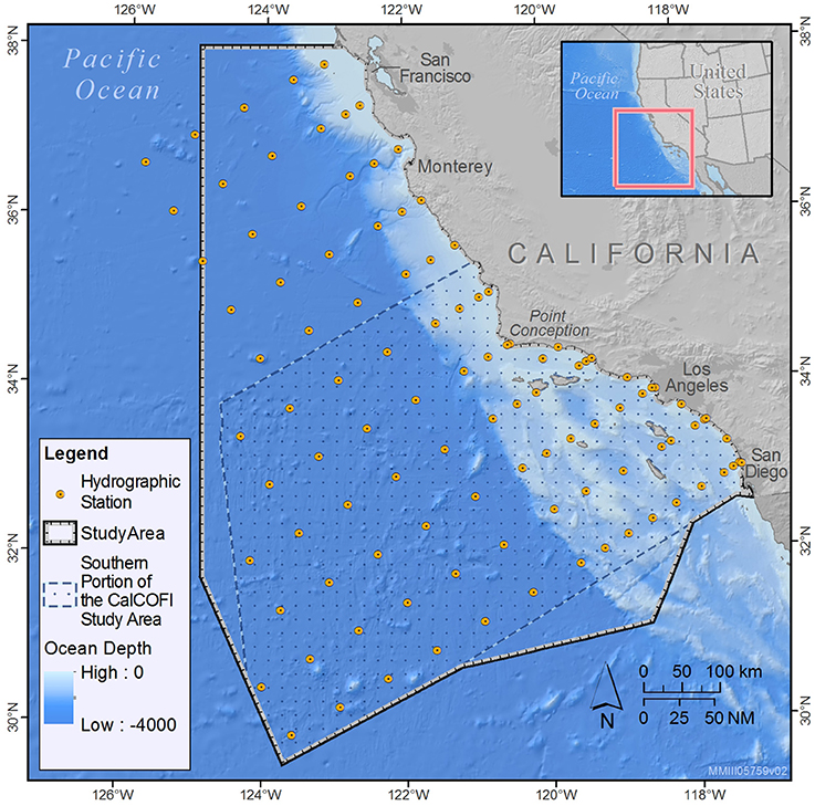
Figure 1. CalCOFI sampling stations (yellow circles) and the approximate 385,460 km² study area (black bold line) used to develop the winter/spring species distribution models presented in this study. The study area was clipped at 125°W longitude to reflect the lack of systematic survey effort west of this line in winter/spring. Also shown is the approximate 238,495 km² southern portion of the CalCOFI study area (hashed area encompassed by the dashed blue line) used by Douglas et al. (2014) and Campbell et al. (2015) to develop line-transect density estimates. The southern boundary roughly follows the Unites States/Mexico border and is consistent with that used by Becker et al. (2016) to develop the summer/fall estimates used for comparison in this study.

Cetacean sighting data used to build the habitat-based density models were collected during quarterly cruises conducted from 2005 to 2015 using systematic line-transect methods (Buckland et al., 2001). Five different research vessels were used during the survey period, but Douglas et al. (2014) found no significant difference in perpendicular distance to transect line for vessels with varying platform height. All surveys were conducted in passing mode (i.e., when a cetacean/cetacean group is sighted the ship continues on course and is not diverted to the vicinity of the sighting) with two dedicated observers searching for cetaceans using unaided eye and 7 × 50 handheld binoculars. Sighting, group size estimates, effort, and weather data were collected and recorded on paper forms and later entered into an electronic record. Detailed descriptions of the survey protocol can be found in Douglas et al. (2014).

Data Processing and Habitat Variables

Samples for modeling were created by dividing transects into approximate 5 km segments of continuous survey effort as described by Becker et al. (2010). To maximize samples sizes for estimation of the detection function, all data collected in Beaufort sea states 0–5 while observers were systematically searching for marine mammals (“on-effort”) were used. To develop the habitat-based density models, only the systematic effort during transits between the CalCOFI stations was included. Species-specific sighting information (number of sightings, mean group size) were assigned to each segment, and habitat data were obtained based on the segment's geographical midpoint.

Products of the Regional Ocean Modeling System (ROMS) from the U.C. Santa Cruz Ocean Modeling and Data Assimilation group (Moore et al., 2011) were used as dynamic predictors to enable comparisons to recent summer/fall SDMs (Becker et al., 2016). The dynamic predictors are served at 10 km spatial resolution (i.e., 100 km²). We used 8-day running average composites centered on the date of each survey segment to provide consistent representation of average survey-day conditions and to ensure consistency with the Becker et al. (2016) summer/fall habitat models. Both the “UCSC ROMS reanalysis” (1990–2010) and the “UCSC ROMS near-real-time” (2011–2015) outputs were used. Only those predictors consistent between the two ROMS outputs were used: sea surface temperature (SST) and its standard deviation [sd(SST)], mixed layer depth, potential energy anomaly (PEA, the work per unit volume required to redistribute the mass in a complete mixing to a depth of 300 m, providing a robust measure of stratification), sea surface height (SSH; with a calibration factor applied to the near-real-time data to match the historical reanalysis dataset), and sd(SSH). Bathymetric variables including depth, slope, and aspect were derived from ETOPO1 (Amante and Eakins, 2009), a 1 arc-min global-relief model. Slope was calculated using ArcGIS Spatial Analyst (Version 10.1, ESRI).

Modeling Methods

A multi-stage modeling approach was implemented to help reduce bias in the density estimates generated from the habitat models. Conducting surveys in passing mode limits the ability of observers to positively identify species, resulting in large numbers of sightings that are not recorded to the species level. Whale blows can be observed at greater distances and in rougher seas than most identifying characteristics, leading to a high proportion of “unidentified large whale” sightings. Distinguishing between short-beaked and long-beaked common dolphins is difficult even at moderate distances (Jefferson et al., 2015), and when observers could not positively identify common dolphin subspecies, the sightings were conservatively recorded as Delphinus spp. Omitting these unidentified animals would result in a severe underestimation of animal density; therefore, we applied correction factors to account for unidentified animals when estimating density in our models. Since more distant animals are more likely to remain unidentified, this approach required the fitting of detection functions for taxonomically pooled species groups that included both unidentified and identified species (e.g., Delphinus spp. and both of the Delphinus subspecies). Our modeling approach was as follows: (1) generate detection functions based on the pooled species groups, (2) develop species-specific correction factors to account for the high proportion of unidentified animals, and (3) build species-specific habitat models and generate density estimates that incorporated the correction factors derived in steps 1 and 2. These steps are described in more detail below.

Step 1: Fit Detection Functions and Estimate Effective Strip Width (ESW)

Given the influence of Beaufort sea state on detectability (Barlow et al., 2001, 2011a; Barlow, 2015), we generated detection functions with Beaufort sea state as a covariate from the full (year-round) 2005–2015 CalCOFI data set (Buckland et al., 2001; Marques et al., 2007) using the R packages mrds (v. 2.1.16) and Distance (v. 0.9.6). Beaufort sea state 0 was combined with Beaufort 1 because of small sample sizes in Beaufort sea state 0. To ensure statistically robust detection functions for short-beaked common dolphin and humpback whale, and to ensure consistency with the correction factors derived to account for unidentified animals (see step 2 below), we pooled all Delphinus spp. and all large whale sightings, respectively.

Detection functions were fit with half-normal and hazard-rate key functions with no adjustment terms, and Akaike's information criterion (AIC; Akaike, 1973) and visual inspection of the detection plots (Thomas et al., 2010) were used to select the best model. Species-specific and segment-specific estimates of ESW were then incorporated into the models based on the recorded sea state conditions on that segment. Prior to modeling, sighting data were truncated at the species-specific truncation distances used to estimate ESW.

Step 2: Derive Correction Factors to Account for Unidentified Animals

The use of passing mode during the CalCOFI surveys resulted in a large number of unidentified large whales and Delphinus spp. (either D. delphis delphis or D. delphis bairdii; Table 1), which would result in a downward bias in estimated encounter rates of humpback whales and short-beaked common dolphins. Therefore, we applied a correction factor to take into account that a subset of the unidentified individuals were actually humpback whales and short-beaked common dolphins. The correction factor c was estimated from the same sighting data used to estimate the detection function for each species group, according to the simplified formula:

$\begin{array}{ll}c=1+\frac{t_{unid}}{t_{tgt}+t_{oth}}& (1)\end{array}$

where t_tgt is the number of individuals identified as the target species (humpback whale or short-beaked common dolphin), t_oth is the number of individuals identified as other species within the broader species group, and t_unid is the number of unidentified individuals in that species group.

TABLE 1

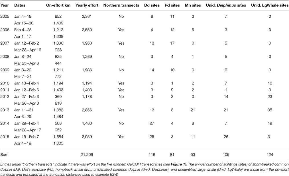
Table 1. CalCOFI winter/spring survey data used to develop the habitat-based density models; on-effort km reflects the distance covered while two observers were on-effort on the main transects located roughly perpendicular to the coast in sea states ≤ 5.

We also examined whether the correction factor varied by Beaufort sea state, due to potential differences in detectability (Barlow et al., 2001, 2011a; Barlow, 2015). For the humpback whale model, higher multipliers were associated with higher sea states because the proportion of unidentified whales increased with increasing sea state. For the short-beaked common dolphin model, the multiplier was greater in lower sea states—likely because of a confounding effect of larger estimated group sizes in lower sea states; therefore, we used a uniform correction factor across all sea states for Delphinus. To correct for group size bias in the resulting short-beaked common dolphin density estimates, we used the “expected group size” based on regressing the logarithm of observed group size vs. perpendicular sighting distance (Buckland et al., 2001; Thomas et al., 2010).

Step 3: Develop Habitat Models and Estimate Density

Generalized Additive Models (GAMs; Hastie and Tibshirani, 1990) were developed in R (v. 3.1.1; R Core Team, 2014) using the package mgcv (v. 1.8-3, Wood, 2011), which includes cross-validation as part of the model selection process. Methods largely followed those described in Becker et al. (2016), but pertinent aspects are summarized here. Restricted maximum likelihood (REML) was used to optimize the parameter estimates as Marra and Wood (2011) found REML to perform better than generalized cross validation. Although mgcv is robust to correlation among predictor variables (termed “concurvity”; Wood, 2011), we found correlations among the predictor variables in our study to be <0.50. Thin-plate regression splines were used for each of the nine potential habitat variables. Automatic term selection (Marra and Wood, 2011), guided by the approximate p-values of each predictor (Wood, 2006, 2011) was used for model selection. We used an iterative process whereby models were initially built with all potential predictors, then non-significant predictors (α = 0.05) were excluded and models re-fit until all predictors were significant.

Two different species-specific modeling frameworks were used, depending on group size characteristics. For Dall's porpoise and humpback whale, species with small and fairly consistent group sizes (average Dall's porpoise group size = 6.26, average humpback whale group size = 1.7), the number of individuals detected on each segment was modeled as the response variable using a Tweedie error distribution to account for overdispersion (Miller et al., 2013). For short-beaked common dolphin, an encounter rate model was developed with the number of sightings per segment modeled as the response variable using a Tweedie error distribution. The expected group size based on the size bias regression method (Buckland et al., 2001; Thomas et al., 2010) was then used in the density equation below.

Density (D, the number of animals per km²) was estimated by incorporating the model results into the line-transect equation (Buckland et al., 2001):

$\begin{array}{ll}{D}_i=\frac{n_i·s_i·c_i}{A_i}& (2)\end{array}$

where i is the segment, n is the number of sightings on segment i, s is the mean or size-bias corrected group size on segment i, c is the correction factor for unidentified animals (derived in step 2 above), based on sea state conditions on segment i, and A is the effective area searched for segment i, corrected for trackline detection probabilities <1:

$\begin{array}{ll}{A}_i=2·L_i·ES{W}_i·g{(0)}_i& (3)\end{array}$

where i is the segment, L is the length of effort segment i, ESW is the effective strip half-width of segment i, and g(0) is the probability of detection on the transect line for segment i. The natural log of the effective area searched was included as an offset in the GAMs.

Following the methods of Becker et al. (2016), we applied segment-specific estimates of g(0) derived by Barlow (2015) from line-transect data collected on large research vessels in the eastern Pacific from 1986–2010. These g(0) estimates are expected to be minimum corrections for the 2-person observer team during CalCOFI surveys, because Barlow (2015) derived these estimates for a 3-person observer team including two observers searching with pedestal-mounted 25 × 150 binoculars.

We used the models to predict density in each cell of a 10 × 10 km grid of the study area for distinct 8-day composites of environmental conditions that spanned the entire survey period. The separate grid predictions were then averaged to produce spatial grids of mean species density and measures of uncertainty within the full CalCOFI study area. The final prediction grids thus provide a “multi-year average” of predicted 8-day cetacean species densities, taking into account the varying oceanographic conditions during the 2005–2015 winter/spring CalCOFI surveys. Sometimes the values of the habitat variables included in the prediction grids can fall outside the range of values used to build the models, potentially leading to model extrapolation errors (Becker et al., 2014). To ensure we were not generating unreasonable predictions, we inspected the range of values for each of the habitat variables included in the full set of 8-day composites and found that some included SST values that were cooler than those used for model development. We thus compared final model predictions based on the full set of 8-day composites to those made on a set that excluded the cooler values. The results were similar, indicating these cool values did not cause extrapolation errors, so we included the full set of 8-day composites for our final model predictions to avoid potential biases. The prediction grid was clipped to the boundaries of the approximate 385,460 km² study area and density predictions were then visually compared to actual sightings made during the winter/spring 2005–2015 surveys.

We assessed potential bias introduced by the habitat-based model by comparing the models' study area abundance estimates to standard line-transect estimates derived from the same dataset used for modeling. The design-based line-transect estimates were derived from the 2005–2015 survey data using Equations (2) and (3) above, but without the inclusion of habitat predictors. Model-based abundance estimates for each grid cell were calculated by multiplying the cell area (in km²) by the predicted species density, exclusive of any portions of the cells located outside the study area or on land. Area calculations were completed using the packages geosphere and gpclib in R (version 2.15.0, R Core Team, 2014). The model-based abundance estimates for the entire study area were calculated as the sum of the individual grid cell abundances.

Seasonal Comparison

To examine seasonal differences in density and distribution, we compared our winter/spring model-based abundance estimates and spatially-explicit density predictions with those derived using similar methods from data collected in summer/fall (July–November) during seven systematic ship surveys conducted by NOAA Fisheries Southwest Fisheries Science Center from 1991–2009 (Becker et al., 2016). These habitat models and the underlying methodology have been extensively validated using cross validation (Forney, 2000; Forney et al., 2012; Barlow et al., 2009; Becker et al., 2010, 2016), predictions on novel data sets (Barlow et al., 2009; Becker et al., 2012, 2014; Forney et al., 2012; Calambokidis et al., 2015), and expert opinion (Barlow et al., 2009; Forney et al., 2012). Although the study area for the Becker et al. (2016) summer/fall models was larger than our CalCOFI study area, the spatial and temporal resolution of the developed models was identical, and similar habitat predictors were used. Thus, a comparison of abundance estimates and spatial patterns within the geographic area of overlap between the two studies can provide insights into potential seasonal changes in species distribution and density in that region. To enable this comparison, we re-calculated model-based abundance estimates for the Becker et al. (2016) summer/fall models within the present CalCOFI study area and examined patterns of species abundance and distribution relative to those identified for winter/spring in the present study.

Results

A total of 21,206 km of on-effort data from 20 CalCOFI surveys conducted during January to April in 2005–2015 were used to develop the winter/spring habitat-based density models. The number of sightings varied between years, particularly for humpback whales that had as many as 21 sightings in 2013 and no sightings during the winter/spring surveys in 2007, 2009, and 2012 (Table 1).

Detection Functions

A half-normal model with Beaufort sea state as a covariate provided the best fit to the perpendicular distance data for all three species (Figure 2). The truncation distance for Delphinus spp. was 1.5 km, eliminating 19% of the most distant sightings. This is higher than the recommended percentage of 5–15% (Buckland et al., 2001), but in passing mode group size estimates decreased with increasing distance, suggesting estimation bias at larger distances. Excluding a greater percentage of sightings thus reduced the potential bias in group size estimation. Further, a size bias regression method was used to estimate the expected mean group size within this truncation distance. Truncation distances were 1.3 km for Dall's porpoise (eliminating 13% of the most distant sightings) and 3.6 km for large whales (eliminating 12% of the most distant sightings).

FIGURE 2

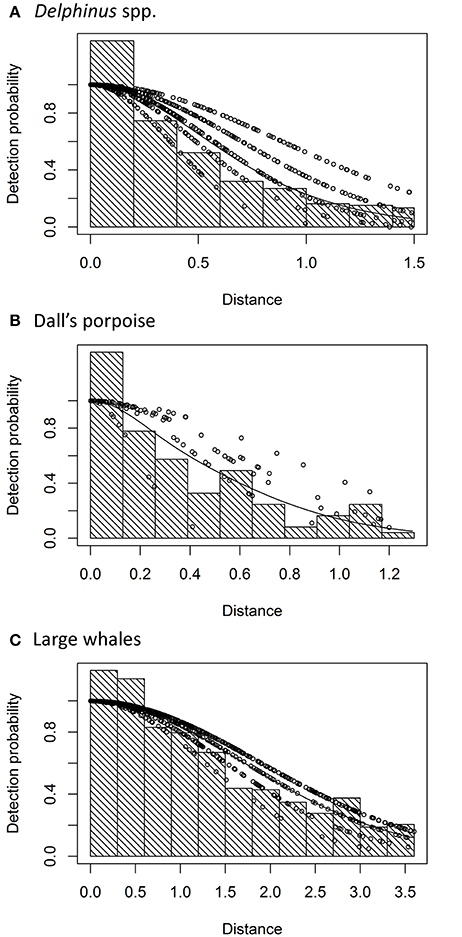
Figure 2. Half-normal detection function models with Beaufort sea state as a covariate fit to perpendicular sighting distances (km) for (A) all Delphinus spp., (B) Dall's porpoise, and (C) all large whales. The histogram shows the distribution of observed perpendicular distances of the sightings, binned to facilitate data analysis (Buckland et al., 2001). The dots are the probability of detection dependent on perpendicular distance and sea state, with lowest sea states on the top (Beaufort 0–1) and highest (Beaufort 5) on the bottom. The solid line shows the average estimated detection function.

Habitat Variables and Model Validation

SST and depth were included in the best models for all three species, but the shape of the relationships differed, reflecting the unique areas of high density for each species within the CalCOFI study area (Figure 3). Short-beaked common dolphin occurrence was highest in the deepest and warmest waters in the study area, with encounters dropping substantially in water temperatures below about 16°C (Figure 3A). The highest numbers of Dall's porpoise occurred in cool waters off the slope, with abundance dropping substantially in water temperatures greater than ~16°C (Figure 3B). Humpback whale numbers were highest in the coolest waters in the study area, occurring primarily over the continental shelf and slope (Figure 3C).

FIGURE 3

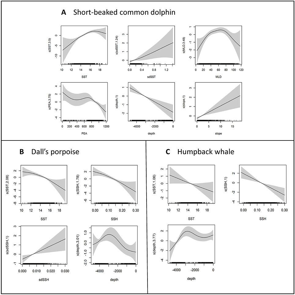
Figure 3. Functional forms for variables included in the final encounter rate (short-beaked common dolphin) or single response (Dall's porpoise and humpback whale) models for (A) short-beaked common dolphin, (B) Dall's porpoise, and (C) humpback whale. Predictor variables in the final models included: SST, sea surface temperature; sdSST, standard deviation of SST; MLD, mixed layer depth; PEA, potential energy anomaly; SSH, sea surface height; sdSSH, standard deviation of SSH; depth, bathymetric depth; and slope, bathymetric slope. The y-axes represent the term's (linear or spline) function, with the degrees of freedom shown in parentheses on the y-axis (linear terms are represented by a single degree of freedom). Zero on the y-axes corresponds to no effect of the predictor variable on the estimated response variable. Scaling of y-axis varies among predictor variables to emphasize model fit. The shading reflects 2× standard error bands (i.e., 95% confidence interval); tick marks (“rug plot”) above the X-axis show data values.

The short-beaked common dolphin encounter rate model explained 18.4% of the deviance. Deviance explained by the single response models was 21.7% for Dall's porpoise and 25.5% for humpback whale. The ratios of observed to predicted density for all species summarized over all years for the entire study area were close to unity for short-beaked common dolphin and humpback whale, and within 8% of unity for Dall's porpoise (Table 2). Similar to previous analyses of summer/fall data, the individual yearly ratios were highly variable, reflecting the reduced predictive ability for any specific year, due in large part to the smaller sample sizes resulting from data stratification (Barlow et al., 2009; Becker et al., 2010; Forney et al., 2012).

TABLE 2

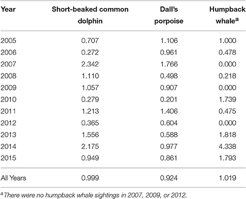
Table 2. Yearly and overall ratios of line-transect over model-predicted density estimates for the total study area as calculated for each segment and summed.

The multi-year average density surface plots captured observed distribution patterns for all three species (Figure 4). Short-beaked common dolphins were broadly distributed throughout the southern portion of the study area, with a notable swath of very low density between higher density regions near the coast and offshore, and highest densities in the southwest portion of the study area (Figure 4A). Predicted densities of Dall's porpoise were highest in the northern portion of the study area, dropping off south of Point Conception (34.4°N; Figure 4B). Model predictions for humpback whale revealed a largely nearshore distribution, with highest densities in the north, particularly in Monterey Bay (36.8°N) and northern coastal waters (Figure 4C).

FIGURE 4

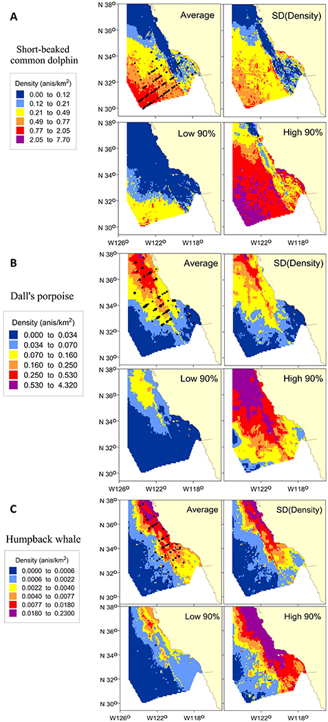
Figure 4. Predicted densities and uncertainty measures from the winter/spring habitat-based density models for (A) short-beaked common dolphin, (B) Dall's porpoise, and (C) humpback whale. Panels show the multi-year average (Average) density based on predicted 8-day cetacean species densities covering the survey periods (winter/spring 2005–2015), as well as the standard deviation of density [SD (Density)], and the 90% confidence limits (Low 90% and High 90%). Density ranges were selected to encompass all values within the confidence limits. Predictions are shown for the study area (385,460 km²). Black dots in the average plots show actual sighting locations from the CalCOFI winter/spring ship surveys for the respective species.

Seasonal Comparison

Multi-year average density plots for summer and fall based on habitat models developed from a separate set of systematic ship survey data by Becker et al. (2016) reveal differences in seasonal distributions for all three species, particularly short-beaked common dolphin (Figure 5). In winter/spring, the highest short-beaked common dolphin densities occurred in the southwest portion of the study area, with decreasing density to the north and east, and a secondary region of higher density nearshore within the Southern California Bight (Figure 5A). This distribution pattern was generally reversed during the summer/fall, with highest densities throughout the Bight and decreasing to the southwest portion of the study area, where some of the lowest densities were predicted. There were low densities and few sightings of short-beaked common dolphins north of Point Conception during the winter/spring surveys, in contrast to high densities and multiple sightings to the north in summer/fall (Figure 5A).

FIGURE 5

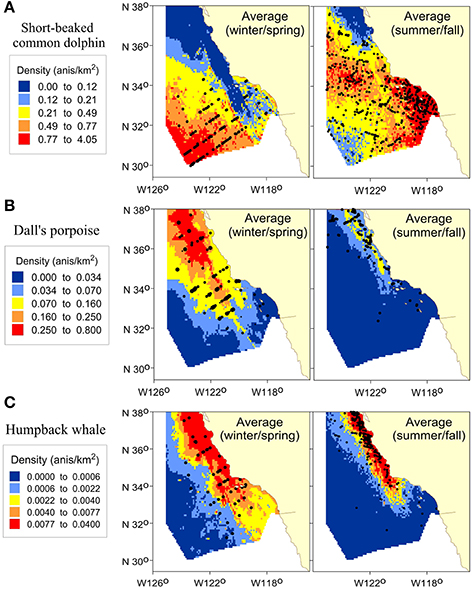
Figure 5. Predicted densities from the winter/spring habitat-based density models from this study compared to summer/fall density predictions based on Becker et al. (2016) for (A) short-beaked common dolphin, (B) Dall's porpoise, and (C) humpback whale. Panels show the multi-year average (Average) density based on predicted 8-day cetacean species densities covering the survey periods for winter/spring (January–April, 2005–2015) and summer/fall (July–November, 1991–2009). Density ranges are those selected for the winter/spring period and are consistent between seasons to emphasize differences. Predictions are shown for the study area (385,460 km²). Black dots show actual sighting locations from the 2005–2015 winter/spring ship surveys and the 1991–2009 summer/fall ship surveys, respectively.

Differences in seasonal distribution patterns of Dall's porpoise were also evident (Figure 5B). Greatest densities occurred north of about 34°N during both seasons, but densities were markedly greater and there was a southward shift in distribution during the winter/spring. The general distribution pattern of humpback whale also differed between seasons, with higher densities south and offshore in winter/spring (Figure 5C).

A comparison of our winter/spring model-based abundance estimates to those derived using similar methods from a separate set of summer/fall surveys conducted in 1991–2009 (Becker et al., 2016) revealed large seasonal differences in the numbers of animals present in the CalCOFI study area (Table 3). The winter/spring abundance estimate for short-beaked common dolphin was 70% lower than the point estimate for summer/fall. For both Dall's porpoise and humpback whale, abundance estimates were substantially greater in winter/spring; almost seven times higher for Dall's porpoise and more than double for humpback whale (Table 3).

TABLE 3

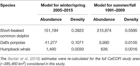
Table 3. Abundance and density estimates derived from habitat-based models for winter/spring (January–April; this study) and for summer/fall (July–November) by Becker et al. (2016) based on line-transect survey data collected during seven systematic ship surveys conducted from July to November between 1991 and 2009.

Discussion

This is the first study to produce spatially-explicit estimates of winter/spring density and distribution for short-beaked common dolphin, Dall's porpoise, and humpback whale off California based on line-transect data collected during these seasons. The overall study area abundance estimates are similar to those derived previously using line-transect analyses (Campbell et al., 2015), but the habitat models provide fine-scale detail in spatial density patterns that are more useful for conservation and management applications. Given the increased use of SDMs to help evaluate and reduce potential risks to cetaceans (e.g., Redfern et al., 2013; U.S. Department of the Navy, 2015), and the documented high degree of seasonal variability in the distribution of cetaceans in the study area (Dohl et al., 1986; Green et al., 1992, 1993; Forney and Barlow, 1998; Becker et al., 2014; Douglas et al., 2014; Henderson et al., 2014; Campbell et al., 2015), it is critical to develop seasonally-explicit SDMs.

Campbell et al. (2015) were able to provide separate line-transect abundance estimates for winter and spring seasons; however, in our study sighting data were not sufficient to develop separate habitat models for the two cool seasons. The use of passing mode on the CalCOFI surveys clearly hampers the ability of observers to positively identify species. Data available for this study included cetacean sightings from 20 separate surveys conducted over an 11-year period, yet sightings were sufficient to develop habitat models for only three species (Table 1). Further, even for these three species the number of sightings available for modeling was limited and did not allow for internal cross validation. Therefore, it is important to continue to collect cetacean survey data during future quarterly CalCOFI surveys to allow model validation and development of more robust models with greater sample sizes. Given the large differences that Campbell et al. (2015) found in abundance between winter and spring for all three species, it also will be important to develop habitat models separately for winter and spring when sufficient sighting data are available.

To help reduce the downward bias associated with the high numbers of unidentified sightings, we applied correction factors to the model-based density estimates for short-beaked common dolphins and humpback whales based on the proportion of unidentified animals within higher taxonomic categories (Delphinus spp. and unidentified large whales, respectively) that were within the truncation distances. While there are alternative methods for assigning species to sightings not fully identified to this taxonomic level, many classification approaches (e.g., Roberts et al., 2016) require large numbers of positive species sightings that were not available in our modeling dataset. In our study, we chose to apply a correction factor to account for the unidentified species sightings; this introduces additional uncertainty in our density estimates but reduces the substantial downward bias that would have otherwise been present.

Species-specific as well as segment-specific estimates of both ESW and g(0) were incorporated into the models based on the recorded viewing conditions on each segment, using coefficients estimated herein for ESW and by Barlow (2015) for g(0). Incorporating these segment-specific correction factors into the habitat models improved the accuracy of the resulting abundance estimates. However, the model-based density estimates we present in this study are still biased-low given that the g(0) estimates were derived based on survey data that used three observers and more powerful binoculars (Barlow, 2015). They do, however, account for a greater number of biases than Campbell et al. (2015), who did not apply corrections for unidentified animals or sea-state specific trackline detection probabilities.

The winter/spring distribution patterns reflected in the multi-year average density plots are generally consistent with past observations, as discussed below for each of the three species.

Short-Beaked Common Dolphin

Forney and Barlow (1998) identified a significant southerly shift in common dolphin distribution off California during winter/spring, with most animals found south of Point Arguello (34.58°N) during the cool seasons. This southern shift in distribution was also noted by Campbell et al. (2015) who also found that all short-beaked common dolphin sightings in winter/spring 2005–2013 were south of 34°N. The distribution pattern reflected in the modeled density predictions was consistent with these studies, as all mid- to high-density regions were predicted south of Point Arguello (Figure 4A).

Based on a statistical comparison of numbers of common dolphins inshore or offshore of the 2,000 m isobath, Forney and Barlow (1998) also identified a significant inshore shift in winter/spring. This inshore shift was also captured in an across-season habitat modeling study (Becker et al., 2014). Campbell et al. (2015) noted that the majority of short-beaked common dolphins observed in winter/spring were found further offshore in pelagic waters off the continental shelf, seemingly contradictory to the findings of Forney and Barlow (1998) and Becker et al. (2014). However, the winter/spring aerial survey data used in the latter two studies did not extend as far offshore as the area where Campbell et al. (2015) identified high concentrations of sightings and where our habitat model estimated mid- to high-densities (Figure 6). Consequently, the winter/spring distribution patterns noted for short-beaked common dolphins in all three of these studies are consistent and show a broad distribution throughout the southern portion of the study area, with a notable swath of very low density between higher density regions near the coast and offshore (Figure 4A). Our winter/spring habitat model for short-beaked common dolphin captured both the near- and offshore regions of higher density, thus helping to resolve the apparent inconsistencies of these past studies.

FIGURE 6

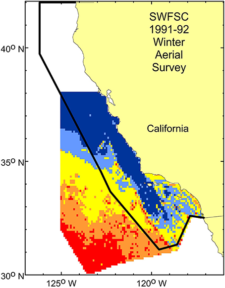
Figure 6. Multi-year average density predictions from the short-beaked common dolphin model shown in Figure 4A overlaid on the Forney and Barlow (1998) aerial survey study area (black solid line), showing that the western edge of the study area is east of the offshore mid- to high-density region identified in this study and noted by Campbell et al. (2015).

The swath of low density running through the study area from northwest to southeast as predicted by the short-beaked common dolphin model (Figure 4A) is a pattern that has not previously been documented for this species. There was concentrated survey effort in this region and the lack of sightings is consistent with the modeled predictions (Figure 4A), so this is not a modeling artifact or sample size limitation. Rather, this band of predicted low density is likely a result of prevailing ocean conditions during winter and spring, when cold water extends from Point Conception southeastward, serving to bifurcate the study area (Figure 7). Short-beaked common dolphins are a warm temperate to tropical species, and based on the models developed here as well as in previous studies (Becker et al., 2010, 2012, 2014, 2016; Forney et al., 2012), densities are greatest when waters are warmest, so there appears to be some avoidance of these areas with cool, upwelled water. Interestingly, genetic differences between short-beaked populations have been identified, with an apparent separate stock occurring in the Southern California Bight (Chivers et al., 2003), corresponding roughly to the nearshore areas of higher density identified by the habitat model (Figure 4A). The separate areas of higher density regions near the coast and offshore identified by the habitat model provide additional support that there may be separate stocks of short-beaked common dolphins off California.

FIGURE 7

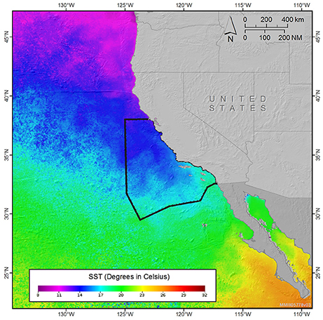
Figure 7. Monthly sea surface temperature composite for a representative cool season period (December 2015) for the U.S. west coast, showing the cool water extending southeast from Point Conception (34.4°N). This cool-water region corresponded to the lowest densities of short-beaked common dolphin shown in Figure 4A, and the general southern extension of Dall's porpoise shown in Figure 4B, coincident with water temperatures of roughly 16°C. The study area boundary is shown with a solid black line. SST data provided courtesy of NOAA CoastWatch: (http://coastwatch.pfeg.noaa.gov/coastwatch/CWBrowser.jsp).

A comparison of density predictions from winter/spring vs. summer/fall habitat models also revealed marked differences for short-beaked common dolphin (Figure 5A). As discussed above, during winter/spring short-beaked common dolphins occur generally south of 34°N, with mid- to high-density regions near the coast and offshore, and highest densities in the southwest portion of the study area (Figure 5A). During summer/fall, some of the lowest densities were predicted for the southwest portion of the study area, with high densities extending well north of 34°N (Figure 5A). The notable difference in seasonal density patterns predicted for short-beaked common dolphin emphasizes the value of developing year-round SDMs for assessing and minimizing potential impacts. This is particularly important in regions with substantial seasonal, interannual, and decadal variability, such as the California Current Ecosystem.

Dall's Porpoise

Statistically significant seasonal shifts in the distribution of Dall's porpoise north and south of Point Arguello have been documented, with animals moving south in winter/spring (Forney and Barlow, 1998). These patterns were more recently confirmed in a study that evaluated across-season habitat models and found that densities of Dall's porpoise were notably higher in the Southern California Bight during winter/spring (Becker et al., 2014). Predicted densities from our winter/spring model are consistent with these past studies and sighting data, with moderate densities of Dall's porpoise south of Point Arguello and in the Bight (Figure 4B).

Distribution patterns based on the winter/spring habitat models were substantially different than those of summer/fall, with the latter predicting very low densities in the Southern California Bight and offshore, and highest predicted densities in a more concentrated band closer to shore at latitudes between 34° and 38°N (Figure 5B). The increase in Dall's porpoise density in waters off Southern California in winter/spring was also noted by Campbell et al. (2015), who found significantly higher densities in winter/spring than summer/fall.

The seasonal distribution patterns shown here are consistent with previous studies that have shown Dall's porpoise to be associated with cool, upwelling-modified waters of the U.S. west coast (Forney, 2000; Becker et al., 2010, 2012). The functional form of the SST variable in the winter/spring model shows numbers of Dall's porpoise dropping rapidly in water temperatures higher than about 16°C (Figure 3B), consistent with findings from previous summer/fall habitat modeling studies based on a different survey data set (Forney, 2000; Becker et al., 2010, 2012, 2014, 2016). As noted above for short-beaked common dolphin, during winter and spring cold water upwelling near Point Conception typically moves to the south/southeast (Figure 7), corresponding well with the southward extension of Dall's porpoise distribution during these seasons (Figure 5B).

Humpback Whale

The majority of humpback whales that feed off California from spring to fall migrate to breed in waters off mainland Mexico and Central America during the winter months (Calambokidis et al., 2000; Barlow et al., 2011b). However, humpback whales have been sighted year-round off California (Dohl et al., 1978, 1983; Forney and Barlow, 1998; Campbell et al., 2015). Forney and Barlow (1998) found that a significantly greater proportion of the humpback whale population was found farther offshore during the winter than the summer, a finding confirmed more recently by Campbell et al. (2015). Our findings are consistent with these results, as the model-predicted distribution pattern for winter/spring extends much further offshore than in the summer/fall (Figure 5C).

Density estimates for humpback whale derived for Southern California waters using line-transect analyses were higher in spring and winter than summer and fall (Campbell et al., 2015), consistent with our model-derived density estimates for the full CalCOFI study area, which were more than double similarly derived model-based estimates for summer/fall (Table 3). This is consistent with previous acoustic monitoring and line-transect studies that showed peak vocalizations and density, respectively, in spring (Helble et al., 2013; Campbell et al., 2015). The documented increase in the number of humpback whales off California in spring, in combination with the predicted offshore distribution pattern, supports a previous hypothesis that both the California feeding population and migrants traveling to areas north of California are present during this season (Forney et al., 1995; Calambokidis et al., 1996).

Large whale species are subject to entanglement in fishing gear off the U.S. west coast (Saez et al., 2013; Feist et al., 2015), and recently the number of humpback whales entangled in fishing gear off central California has increased¹, particularly during spring. To help establish policies to avoid or minimize entanglement risk, there is a need to understand the spatial and temporal overlap of whales and fishing gear. Although the spatial resolution in our current study may be too coarse for evaluating spatial risk of entanglement in nearshore waters, they are the first spatially-explicit models of humpback whale distribution for winter/spring and can provide a foundation for further fine-scale modeling efforts.

Conclusions

The new habitat-based density models developed for short-beaked common dolphin, Dall's porpoise, and humpback whale in this study offer spatially-resolved seasonal densities, in support of the assessment and mitigation of anthropogenic impacts. The models have also expanded our knowledge of seasonal changes in density and distribution patterns of these three species off central and southern California. The spatial extent of the seasonal differences in distribution patterns emphasizes the need to develop winter/spring models for additional species as data permit, and ideally develop separate models for each season. Future studies should evaluate the potential for combining the year-round CalCOFI survey data with sighting data collected during summer and fall of 1991–2014 during the Southwest Fisheries Science Center surveys off the U.S. west coast (Barlow, 2016). Hierarchical Bayesian methods would allow such different datasets to be combined effectively to maximize sample sizes, increase the temporal and spatial coverage of the sighting data, and further improve density estimates and models of seasonal distribution patterns in this highly dynamic ecosystem.

Author Contributions

EB and KF conceived of the work and interpreted the results. EB conducted the analysis with contributions from KF, AG, and RH. BT, AJD, and GC processed the CalCOFI survey data files. GC, KW, and ABD led the marine mammal data collection efforts. JH contributed the survey data. All authors contributed to writing and revising the manuscript, and have approved of the manuscript.

Funding

This project was funded by the Navy, Commander, U.S. Pacific Fleet and by the National Oceanic, and Atmospheric Administration (NOAA), National Marine Fisheries Service (NMFS), Southwest Fisheries Science Center (SWFSC). AG was supported by the Humboldt Foundation.

Conflict of Interest Statement

The authors declare that the research was conducted in the absence of any commercial or financial relationships that could be construed as a potential conflict of interest.

Acknowledgments

We are especially thankful for the hard work and dedication of all the marine mammal observers who collected the CalCOFI survey data used in this study. Christopher Edwards and Andrew Moore (Ocean Sciences Department, University of California, Santa Cruz) provided the ROMS outputs used for modeling, and we are thankful for their continued input and support. This manuscript was improved by the helpful reviews of Dr. Jessica Redfern (Marine Mammal and Turtle Division of SWFSC), Chip Johnson (U.S. Navy, Pacific Fleet), Dr. Leslie New, and Dr. Francesco Ventura.

Footnotes

1. ^http://www.opc.ca.gov/webmaster/ftp/project_pages/whale-entanglement/EntanglementUpdates2014-2016.pdf.

References

Akaike, H. (1973). “Information theory and an extension of the maximum likelihood principle,” in Second International Symposium on Information Theory, eds B. N. Petran and F. Csàaki (Budapest: Akadèemiai Kiadi), 267–281.

Amante, C., and Eakins, B. W. (2009). ETOPO1 1 Arc-Minute Global Relief Model: Procedures, Data Sources and Analysis. Technical Memorandum NESDIS NGDC-24, National Geophysical Data Center, Boulder, CO.

Barlow, J. (2015). Inferring trackline detection probabilities, g(0), for cetaceans from apparent densities in different survey conditions. Mar. Mamm. Sci. 31, 923–943. doi: 10.1111/mms.12205

CrossRef Full Text | Google Scholar

Barlow, J. (2016). Cetacean Abundance in the California Current Estimated from Ship-Based Line-Transect Surveys in 1991-2014. NOAA Administrative Report NMFS-SWFSC LJ-16–J-01.

Barlow, J., Balance, L. T., and Forney, K. A. (2011a). Effective Strip Widths for Ship-Based Line-Transect Surveys of Cetaceans. NOAA Technical Memorandum NMFS-SWFSC-484.

Barlow, J., Calambokidis, J., Falcone, E. A., Baker, C. S., Burdin, A. M., Clapham, P. J., et al. (2011b). Humpback whale abundance in the North Pacific estimated by photographic capture-recapture with bias correction from simulation studies. Mar. Mamm. Sci. 27, 793–818. doi: 10.1111/j.1748-7692.2010.00444.x

CrossRef Full Text | Google Scholar

Barlow, J., Ferguson, M. C., Becker, E. A., Redfern, J. V., Forney, K. A., Vilchis, I. L., et al. (2009). Predictive Modeling of Cetacean Densities in the Eastern Pacific Ocean. NOAA Technical Memorandum NMFS-SWFSC-444.

Barlow, J., Gerrodette, T., and Forcada, J. (2001). Factors affecting perpendicular sighting distances on shipboard line-transect surveys for cetaceans. J. Cetacean Res. Manag. 3, 201–212.

Becker, E. A., Foley, D. G., Forney, K. A., Barlow, J., Redfern, J. V., and Gentemann, C. L. (2012). Forecasting cetacean abundance patterns to enhance management decisions. Endang. Species Res. 16, 97–112. doi: 10.3354/esr00390

CrossRef Full Text | Google Scholar

Becker, E. A., Forney, K. A., Ferguson, M. C., Foley, D. G., Smith, R. C., Barlow, J., et al. (2010). Comparing California Current cetacean-habitat models developed using in situ and remotely sensed sea surface temperature data. Mar. Ecol. Prog. Ser. 413, 163–183. doi: 10.3354/meps08696

CrossRef Full Text | Google Scholar

Becker, E. A., Forney, K. A., Fiedler, P. C., Barlow, J., Chivers, S. J., Edwards, C. A., et al. (2016). Moving towards dynamic ocean management: how well do modeled ocean products predict species distributions? Remote Sens. 8:149. doi: 10.3390/rs8020149

CrossRef Full Text | Google Scholar

Becker, E. A., Forney, K. A., Foley, D. G., Smith, R. C., Moore, T. J., and Barlow, J. (2014). Predicting seasonal density patterns of California cetaceans based on habitat models. Endang. Species Res. 23, 1–22. doi: 10.3354/esr00548

CrossRef Full Text | Google Scholar

Benson, S. R., Eguchi, T., Foley, D. G., Forney, K. A., Bailey, H., Hitipeuw, C., et al. (2011). Large-scale movements and high-use areas of western Pacific leatherback turtles, Dermochelys coriacea. Ecosphere 2, 84. doi: 10.1890/ES11-00053.1

CrossRef Full Text

Bograd, S. J., Checkley, D. A., and Wooster, W. S. (2003). CalCOFI: a half century of physical, chemical, and biological research in the California Current System. Deep Sea Res. Part II 50, 2349–2353. doi: 10.1016/S0967-0645(03)00122-X

CrossRef Full Text | Google Scholar

Briggs, J. C. (1974). Marine Zoography. New York, NY: McGraw-Hill.

Buckland, S. T., Anderson, D. R., Burnham, K. P., Laake, J. L., Borchers, D. L., and Thomas, L. (2001). Introduction to Distance Sampling: Estimating Abundance of Biological Populations. Oxford: Oxford University Press.

Google Scholar

Calambokidis, J., Steiger, G. H., Curtice, C., Harrison, J., Ferguson, M. C., Becker, E. A., et al. (2015). Biologically important areas for selected cetaceans within U.S. waters-West Coast region. Aquat. Mamm. 41, 39–53. doi: 10.1578/AM.41.1.2015.39

CrossRef Full Text | Google Scholar

Calambokidis, J., Steiger, G. H., Evenson, J. R., Flynn, K. R., Balcomb, K. C., Claridge, D. E., et al. (1996). Interchange and isolation of humpback whales off California and other North Pacific feeding grounds. Mar. Mamm Sci. 12, 215–226. doi: 10.1111/j.1748-7692.1996.tb00572.x

CrossRef Full Text | Google Scholar

Calambokidis, J., Steiger, G. H., Rasmussen, K., Urban, R. J., Balcomb, K. C., Ladrón de Guevara, P. P., et al. (2000). Migratory destinations of humpback whales that feed off California, Oregon and Washington. Mar. Ecol. Prog. Ser. 192, 295–304. doi: 10.3354/meps192295

CrossRef Full Text | Google Scholar

Campbell, G. S., Thomas, L., Whitaker, K., Douglas, A. B., Calamboikdis, J., and Hildebrand, J. A. (2015). Inter-annual and seasonal trends in cetacean distribution, density and abundance off Southern California. Deep Sea Res. Part II 112, 143–157. doi: 10.1016/j.dsr2.2014.10.008

CrossRef Full Text | Google Scholar

Chivers, S. J., Le Duc, R. G., and Robertson, K. M. (2003). A Feasibility Study to Evaluate Using Molecular Genetic Data to Study Population Structure of Eastern North Pacific Delphinus Delphis. NOAA Administrative Report NMFS-SWFSC LJ-03–12.

Dohl, T. P., Bonnell, M. L., and Ford, R. G. (1986). Distribution and abundance of common dolphin, Delphinus delphis, in the Southern California Bight: a quantitative assessment based upon aerial transect data. Fish. Bull. 84, 333–343.

Dohl, T. P., Guess, R. C., Duman, M. L., and Helm, R. C. (1983). Cetaceans of Central and Northern California, 1980–1983: Status, Abundance, and Distribution. Prepared for Pacific OCS Region, Minerals Management Service, U.S. Department of the Interior, Contract No. 14-12-0001-29090, NTIS Catalog No. PB85-183861.

Dohl, T. P., Norris, K. S., Guess, R. C., Bryant, J. D., and Honig, M. W. (1978). Summary of Marine Mammal and Seabird Surveys of the Southern California Bight Area, 1975-78, Vol. III: Investigators' Reports, Part II: Cetacea of the Southern California Bight. Final Report to the Bureau of Land Management, NTIS Catalog No. PB81–248189.

Douglas, A. B., Calambokidis, J., Munger, L. M., Soldevilla, M. S., Ferguson, M. C., Havron, A. M., et al. (2014). Seasonal distribution and abundance of cetaceans off southern California estimated from CalCOFI cruise data from 2004 to 2008. Fish. Bull. 112, 197–220. doi: 10.7755/fb.112.2-3.7

CrossRef Full Text | Google Scholar

Doyle, R. F. (1985). Biogeographical Studies of Rocky Shore Near Point Conception, California. Ph.D. dissertation, University of California, Santa Barbara, CA.

Feist, B., Bellman, M. A., Becker, E. A., Forney, K. A., Ford, M. J., and Levin, P. S. (2015). Potential Overlap between Cetaceans and Commercial Groundfish Fleets that Operate in the California Current Large Marine Ecosystem. NOAA Professional Papers, NMFS Scientific Publications Office, NOAA, 17.

Forney, K. A. (2000). Environmental models of cetacean abundance: reducing uncertainty in population trends. Conserv. Biol. 14, 1271–1286. doi: 10.1046/j.1523-1739.2000.99412.x

CrossRef Full Text | Google Scholar

Forney, K. A., and Barlow, J. (1998). Seasonal patterns in the abundance and distribution of California cetaceans, 1991-1992. Mar. Mamm. Sci. 14, 460–489. doi: 10.1111/j.1748-7692.1998.tb00737.x

CrossRef Full Text | Google Scholar

Forney, K. A., Barlow, J., and Carretta, J. V. (1995). The abundance of cetaceans in California waters. Part II: aerial surveys in winter and spring of 1991 and 1992. Fish. Bull. 93, 15–26.

Forney, K. A., Ferguson, M. C., Becker, E. A., Fiedler, P. C., Redfern, J. V., Barlow, J., et al. (2012). Habitat-based spatial models of cetacean density in the eastern Pacific Ocean. Endang. Species Res. 16, 113–133. doi: 10.3354/esr00393

CrossRef Full Text | Google Scholar

Gilles, A., Adler, S., Kaschner, K., Scheidat, M., and Siebert, U. (2011). Modelling harbor porpoise seasonal density as a function of the German Bight environment: implications for management. Endang. Species Res. 14, 157–169. doi: 10.3354/esr00344

CrossRef Full Text | Google Scholar

Gilles, A., Viquerat, S., Becker, E. A., Forney, K. A., Geelhoed, S. C. V., Haelters, J., et al. (2016). Seasonal habitat-based density models for a marine top predator, the harbor porpoise, in a dynamic environment. Ecosphere 7, 1–22. doi: 10.1002/ecs2.1367

CrossRef Full Text | Google Scholar

Goetz, K. T., Montgomery, R. A., Ver Hoef, J. M., Hobbs, R. C., and Johnson, D. S. (2012). Identifying essential summer habitat of the endangered beluga whale Delphinapterus leucas in Cook Inlet, Alaska. Endang. Species Res. 16, 135–147. doi: 10.3354/esr00394

CrossRef Full Text | Google Scholar

Green, G. A., Brueggeman, J. J., Grotefendt, R. A., Bowlby, C. E., Bonnell, M. L., and Balcomb, K. C. I. I. I. (1992). “Cetacean distribution and abundance off Oregon and Washington, 1989-1990,” in Oregon and Washington Marine Mammal and Seabird Surveys, ed J. J. Brueggeman (U.S. Department of the Interior, Minerals Management Service, contract 14-12-0001-30426, OCS Study MMS 91-0093), 1–100.

Google Scholar

Green, G. A., Grotefendt, R. A., Smultea, M. A., Bowlby, C. E., and Rowlett, R. A. (1993). Delphinid Aerial Surveys in Oregon and Washington Offshore Waters. Final report prepared for NMFS, National Marine Mammal Laboratory, AFSC, 7600 Sand Point Way NE, Contract No. 50ABNF200058, Seattle, WA.

Hammond, P. S., Mcleod, K., Berggren, P., Borchers, D. L., Burt, L., Ca-adas, A., et al. (2013). Cetacean abundance and distribution in European Atlantic shelf waters to inform conservation and management. Biol. Conserv. 164, 107–122. doi: 10.1016/j.biocon.2013.04.010

CrossRef Full Text | Google Scholar

Hastie, T. J., and Tibshirani, R. J. (1990). Generalized Additive Models, Vol. 43. Boca Raton, FL: Chapman & Hall/CRC.

Hazen, E. L., Palacios, D. M., Forney, K. A., Howell, E. A., Becker, E. A., Hoover, A. L., et al. (2016). WhaleWatch: a dynamic management tool for predicting blue whale density in the California current. J. Appl. Ecol. doi: 10.1111/1365-2664.12820. [Epub ahead of print].

CrossRef Full Text | Google Scholar

Helble, T. A., D'Spain, G. L., Campbell, G. S., and Hildebrand, J. A. (2013). Calibrating passive acoustic monitoring: correcting humpback call detections for site-specific and time-dependent environmental characteristics. J. Acoust. Soc. Am. 134, EL400–EL406. doi: 10.1121/1.4822319

PubMed Abstract | CrossRef Full Text | Google Scholar

Henderson, E. E., Forney, K. A., Barlow, J., Hildebrand, J. A., Douglas, A. B., Calambokidis, J., et al. (2014). Effects of fluctuations in sea-surface temperature on the occurrence of small cetaceans off Southern California. Fish. Bull. 112, 159–177. doi: 10.7755/FB.112.2-3.5

CrossRef Full Text | Google Scholar

Hobday, A. J., Hartog, J. R., Timmis, T., and Fielding, J. (2010). Dynamic spatial zoning to manage southern bluefin tuna capture in a multi-species longline fishery. Fish. Oceanogr. 19, 243–253. doi: 10.1111/j.1365-2419.2010.00540.x

CrossRef Full Text | Google Scholar

Jefferson, T. A., Webber, M. A., and Pitman, R. L. (2015). Marine Mammals of the World: A Comprehensive Guide to Their Identification, 2nd Edn. London: Academic Press.

Louzao, M., Hyrenbach, K. D., Arcos, J. M., Abelló, P., Gil de Sola, L., and Oro, D. (2006). Oceanographic habitat of an endangered Mediterranean Procellariiform: implications for marine protected areas. Ecol. Appl. 16, 1683–1695. doi: 10.1890/1051-0761(2006)016[1683:OHOAEM]2.0.CO;2

PubMed Abstract | CrossRef Full Text | Google Scholar

Marques, T. A., Thomas, L., Fancy, S. G., and Buckland, S. T. (2007). Improving estimates of bird density using multiple covariate distance sampling. Auk 124, 1229–1243. doi: 10.1642/0004-8038(2007)124[1229:IEOBDU]2.0.CO;2

CrossRef Full Text | Google Scholar

Marra, G., and Wood, S. (2011). Practical variable selection for generalized additive models. Comput. Stat. Data Anal. 55, 2372–2387. doi: 10.1016/j.csda.2011.02.004

CrossRef Full Text | Google Scholar

Miller, D. L., Burt, M. L., Rexstad, E. A., Thomas, L., and Gimenez, O. (2013). Spatial models for distance sampling data: recent developments and future directions. Methods Ecol. Evol. 4, 1001–1010. doi: 10.1111/2041-210X.12105

CrossRef Full Text | Google Scholar

Moore, A. M., Arango, H. G., Broquet, G., Edwards, C. A., Veneziani, M., Powell, B. S., et al. (2011). The regional ocean modeling system (ROMS) 4-dimensional variational data assimilation systems. II: performance and application to the California current system. Prog. Oceanogr. 91, 50–73. doi: 10.1016/j.pocean.2011.05.003

CrossRef Full Text | Google Scholar

Newman, W. A. (1979). “California transition zone: significance of short-range endemics,” in Historical Biogeography, Plate Tectonics, and the Changing Environment, eds J. Gray and A. J. Boucot (Corvallis, OR: Oregon State University Press), 399–416.

R Core Team (2014). R: A Language and Environment for Statistical Computing R. Vienna: Foundation for Statistical Computing. Available online at: www.R-project.org/

Redfern, J. V., McKenna, M. F., Moore, T. J., Calambokidis, J., DeAngelis, M. L., Becker, E. A., et al. (2013). Assessing the risk of ships striking large whales in marine spatial planning. Conserv. Biol. 27, 292–302. doi: 10.1111/cobi.12029

PubMed Abstract | CrossRef Full Text | Google Scholar

Roberts, J. J., Best, B. D., Mannocci, L., Fujioka, E., Halpin, P. N., Palka, D. L., et al. (2016). Habitat-based cetacean density models for the U.S. Atlantic and Gulf of Mexico. Sci. Rep. 6:22615. doi: 10.1038/srep22615

PubMed Abstract | CrossRef Full Text | Google Scholar

Saez, L., Lawson, D., DeAngelis, M., Petras, E., Wilin, S., and Fahy, C. (2013). Understanding the Co-Occurrence of Large Whales and Commercial Fixed Gear Fisheries Off the West Coast of the United States. NOAA Technical Memorandum NMFS, NOAA-TM-NMFS-SWR-044.

Soldevilla, M. S., Wiggins, S. M., Calambokidis, J., Douglas, A. B., Oleson, E. M., and Hildebrand, J. A. (2006). Marine mammal monitoring and habitat investigations during CalCOFI surveys. CalCOFI Rep. 47, 79–91.

Google Scholar

Thomas, L., Buckland, S. T., Rexstad, E. A., Laake, J. L., Strindberg, S., Hedley, S. L., et al. (2010). Distance software: design and analysis of distance sampling surveys for estimating population size. J. Appl. Ecol. 47, 5–14. doi: 10.1111/j.1365-2664.2009.01737.x

PubMed Abstract | CrossRef Full Text | Google Scholar

U.S. Department of the Navy (2015). U.S. Navy's Marine Species Density Database for the Pacific Ocean. NAVFAC Pacific Technical Report, Naval Facilities Engineering Command Pacific, Pearl Harbor, HI, 486.

Valentine, J. W. (1973). Evolutionary Paleoecology of the Marine Biosphere. Englewood Cliffs, NJ: Prentice-Hall.

Google Scholar

Wood, S. N. (2006). Generalised Additive Models–An Introduction with R. Boca Raton, FL: Chapman and Hall/CRS.

Google Scholar

Wood, S. N. (2011). Fast stable restricted maximum likelihood and marginal likelihood estimation of semiparametric Generalized Linear Models. J. R. Statist. Soc. Ser. B 73, 3–36. doi: 10.1111/j.1467-9868.2010.00749.x

CrossRef Full Text | Google Scholar