Estimates of Water-Column Nutrient Concentrations and Carbonate System Parameters in the Global Ocean: A Novel Approach Based on Neural Networks

Introduction

The ocean is under increasing stress (Gruber, 2011; Gattuso et al., 2015). Given this context of a rapidly changing ocean, it is crucial to reinforce the observation capability of biogeochemical variables and develop ways of measuring or estimating new ones (Claustre et al., 2010; Gruber et al., 2010b). This is required not only for monitoring ongoing changes, but also to gain a better understanding of key biogeochemical processes and for reducing uncertainties in budgets of major elements (e.g., carbon, oxygen, nitrogen, phosphorus, and silicium).

Reaching the goal of an improved global observation system for biogeochemical variables primarily relies on enhancing the spatio-temporal resolution of measurements. Historically, marine biogeochemical observations have been conducted from ships either taking discrete water samples followed by laboratory analyses (e.g., Global Ocean Ship-based Hydrographic Investigations Panel, GO-SHIP program; Talley et al., 2016), or conducting continuous measurements of surface-water properties. These approaches have been and still remain essential as their estimates generally have the highest accuracies. Such measurements have been assembled into global databases (e.g., GLODAPv2; Key et al., 2015; Olsen et al., 2016), which are a key resource for making budgets of chemical elements, directly from available measurements (Takahashi et al., 2009) or indirectly through specific innovative methods (Landschützer et al., 2013, 2014, 2016), conducting climate change research (Le Quéré et al., 2015) and biogeochemical modeling (e.g., use of data for model initialization and/or validation; Doney et al., 2009; Ilyina et al., 2013). The ship-based sampling mode has one major limit, i.e., coarse spatio-temporal resolution and resulting under-sampling of marine biogeochemical properties. This severely limits the understanding of fundamental processes and the accurate documentation of ongoing changes, especially at some critical scales (e.g., seasonal, regional).

Over the last two decades, observation technologies such as autonomous platforms have matured (e.g., profiling floats and gliders equipped with biogeochemical sensors; Johnson et al., 2009, 2013, 2016). Robotic observation now provides a reliable complement to ship-based sampling that can be used to cost-effectively densify the acquisition of marine biogeochemical properties (Johnson et al., 2009). Among such observation systems, the recently launched Biogeochemical-Argo (BGC-Argo) network offers a promising approach for the global coverage and spatio-temporal resolution of biogeochemical properties (Johnson and Claustre, 2016). The biogeochemically-relevant variables amenable to systematic and reliable acquisition with robotic observation systems presently include concentrations of oxygen (O₂) and their number increases rapidly (Johnson et al., 2015). More generally, O₂ concentration is the most mature measurement, and could be easily implemented on all types of profiling floats (Gruber et al., 2010a) including those of the BGC-Argo network.

Oxygen optode sensors have been progressively implemented on profiling floats since the early 2000s, and have thus opened a new area of research (e.g., Körtzinger et al., 2004; Martz et al., 2008; Riser and Johnson, 2008). Strong efforts have been devoted toward the improvement of the long-term reliability and accuracy of autonomous O₂ measurements on profiling floats. A crucial step is the possibility of frequently calibrating optodes by recording O₂ in air when the float surfaces (Bittig and Körtzinger, 2015; Johnson et al., 2015; Bushinsky et al., 2016). Such a calibration can be done for each profile and throughout the float's lifetime, improves the precision and accuracy of O₂ measurements to within 0.2 and 1 %, respectively (Bittig and Körtzinger, 2015), which accuracy is comparable to that of the reference Winkler titration technique. Water column O₂ concentration can therefore be globally monitored at the biogeochemically relevant spatial and temporal resolutions. This will move O₂, which required specialized measurements until now, among the key standard oceanographic variables.

In the present study, we develop a new approach with which the expected increased densification of O₂ measurements in the near future could be used to support new studies related to seven key biogeochemical variables, i.e., concentrations of three dissolved inorganic macronutrients (nitrate, phosphate, and silicate) and four parameters of the carbonate system (total alkalinity, dissolved inorganic carbon, pH on the total scale, and partial pressure of CO₂). Because O₂ concentration is a variable that reflects both phytoplankton production and community respiration processes, the first-order relationships which link O₂, nutrients and inorganic carbon are rather well-constrained through Redfield stoichiometry (Redfield, 1934, 1958). These intrinsic relationships have been used to develop, from regional to global scales, multiple linear regression, or neural network approaches that link O₂ and simultaneously acquired variables (e.g., pressure, temperature, salinity) to biogeochemical variables, in particular parameters of the carbonate system (Juranek et al., 2011; Velo et al., 2013; Carter et al., 2016; Williams et al., 2016). These relationships could be used as transfer functions to convert dense fields of O₂ (and associated variables) into corresponding fields of biogeochemical variables of interest. This represents a way to cost-effectively populate, spatially, and temporally, the previously loosely resolved fields of these variables.

Such transfer functions represent a potential approach to profit from the upcoming numerous accurate measurements of O₂ (from profiling floats), which are expected to be routine soon, to derive properties or variables that are difficult or costly to acquire. To be useful, these functions must provide “predicted” variables with relatively high accuracy, and they should be as generic as possible (i.e., ideally of global applicability). Among the different possible methods for developing such transfer functions, artificial neural networks are an attractive tool as these powerful methods can be used for approximating any differentiable and continuous functions and thus allow to model complex and non-linear relationships (Hornik et al., 1989; Lek and Guégan, 1999). As a consequence, neural networks have already been largely used for biogeochemical and geophysical applications (e.g., Ward and Redfern, 1999; Friedrich and Oschlies, 2009; Jamet et al., 2012; Ben Mustapha et al., 2013). More recently, neural networks have been used successfully to retrieve the vertical distribution of biogeochemical variables at the global scale using as input the geolocation variables, providing a single global transfer function handling boundary issues compared to regional-based functions (Sauzède et al., 2015, 2016).

The present study takes advantage of the simultaneous release of the GLODAPv2 database (Olsen et al., 2016) and the planning of the BGC-Argo program (Johnson and Claustre, 2016). The two observational systems and resulting databases are highly complementary, and new approaches can be developed to synergistically use their respective strengths, i.e., measurement accuracy for GLODAPv2, and spatio-temporal coverage for BGC-Argo, with a specific emphasis on O₂ measurements. We thus focus in this study on the development of global neural network-based transfer functions using O₂ as a primary input to retrieve nutrient concentrations and carbonate system parameters in the water column down to 8,000 m. Hereinafter, we refer to our method as CANYON, for CArbonate system and Nutrients concentration from hYdrological properties and Oxygen using a Neural network.

Material and Methods

The GLODAPv2 Database

The Global Ocean Data Analysis Project version 2 (GLODAPv2) was an effort from the international community to consolidate all data from ocean bottle samples collected as part of many oceanic cruises (Olsen et al., 2016). The GLODAPv2 database (available at http://cdiac.ornl.gov/oceans/GLODAPv2/) provides a single high-quality internally consistent global data product that contains CO₂-relevant ocean interior measurements from ship-based surveys. The GLODAPv2 database includes samples of core variables such as salinity, oxygen, macronutrients, and seawater CO₂ chemistry from 724 oceanic cruises. In this study, we focused on seven variables representative of the macronutrients and of the seawater carbonate system: nitrate (NO₃⁻), phosphate (PO₄³⁻), silicate (Si(OH)₄), pH on the total scale (pH_T), total alkalinity (A_T), total dissolved inorganic carbon (C_T), and partial pressure of CO₂ (pCO₂). Note that we estimated this last variable from the A_T and C_T measurements available in GLODAPv2 (see details below).

Initially, GLODAPv2 was instigated to prepare a unified, bias-corrected interior ocean data product. Thus, a high quality control, QC, based on two steps (i.e., primary and secondary QC) was applied to each data (Olsen et al., 2016). The primary QC was carried out following routines outlined in Sabine et al. (2005) and Tanhua et al. (2010), essentially based on inspection of property-property plots. The secondary QC for salinity, oxygen, nutrients, C_T, and A_T was more complex, and carried out through crossover (i.e., comparing data where two different cruises crossed or came close to each over) and inversion analyses (i.e., calculation of corrections required to minimize all cruise-by-cruise offsets). This two step-based method was introduced by Gouretski and Jancke (2000) and Johnson et al. (2001). For the secondary QC applied to the GLODAPv2 database, the crossover offsets were calculated using the running-cluster crossover routine (Tanhua et al., 2010), with data from beneath 2,000 m to minimize effects of real variations. For pH_T, crossover analysis was not possible because data only exist for a small fraction of the cruises. To pass the secondary QC, pH_T measurements had to be concomitant with C_T and/or A_T for calculating offsets (see details in Olsen et al., 2016). For Mediterranean Sea data, the secondary QC always failed because none of the cruises inside the Mediterranean had an overlap with other cruises (e.g., outside the Mediterranean) thus preventing the crossover analysis. Hence, only “high-quality” GLODAPv2 data that passed the secondary QC were used to train and validate the CANYON methods except for the Mediterranean Sea where we used data that only passed the primary QC.

The subset of the GLODAPv2 database used for our study (i.e., the data that passed the secondary QC, except for the Mediterranean Sea data as explained above) contained 37,863 concurrent profiles of water-column (from the surface to a maximum sample depth of 8,000 m) hydrological properties together with nutrients concentration and/or parameters of the carbonate system (see Figure 1). These data were collected between 1972 and 2013 and were representative of the diversity of oceanic regions, i.e., 25 % were collected in the North Atlantic, 10 % in the South Atlantic, 22 % in the North Pacific, 12 % in the South Pacific, 10 % in the Indian Ocean, 13 % in the Southern Ocean, 7 % in the Arctic Ocean, and ~0.2 % in the Mediterranean Sea (geographic boundaries are provided in Figure S1). On the temporal scale, most of the data were acquired since the 1990's and more data were available for the spring and summer months (Figure S2). There was a sampling bias according to latitude as data from autumn and winter months (i.e., December to March for the Northern hemisphere, and May to August for the Southern hemisphere) were less represented at high than low latitudes (i.e., >45° North and South, respectively) in the GLODAPv2 database (Figure S2).

FIGURE 1

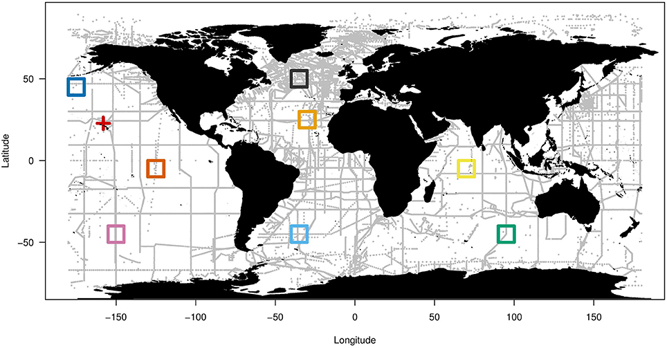
Figure 1. Geographic distribution of the 37,863 stations (gray dots) used in this study (from the GLODAPv2 database; Olsen et al., 2016). For each station, concurrent samples of temperature, salinity, concentrations of O₂, and nutrients and/or carbonate system parameters were analyzed. The red cross indicates the location of the Hawaiian Time Series (HOT, used in Section Example of Application: Illustration with HOT Database). The eight colored boxes delineate the eight independent zones of which data were not included in the training and validation of the neural network.

All the data used to train and validate CANYON were measurements recorded in the GLODAPv2 database, except the pCO₂ estimates that we calculated from A_T and C_T measurements using the R package “seacarb” (Gattuso et al., 2015, 2016). The carbonate system parameters were computed using the carbonic acid dissociation constants of Lueker et al. (2000), the hydrogen fluoride dissociation constant of Perez and Fraga (1987), the dissociation constant for bisulfate of Dickson (1990), and a ratio of total boron to salinity derived from Uppström (1974). In situ measurements of salinity, temperature, hydrostatic pressure as well as the concentrations of PO₄³⁻ and Si(OH)₄ were used to calculate pCO₂. When not available in the GLODAPv2 database, the concentrations of PO₄³⁻ and Si(OH)₄ were estimated using our CANYON algorithm (see associated accuracies in Section Overall CANYON Performance).

For the neural network development, vertical profiles of nutrients and carbonate system parameters from eight independent zones of the GLODAPv2 database (squares of 10° latitude × 10° longitude) were first removed from the general database to provide a more “independent data set” used for an independent validation of the algorithm developed in this study. These zones were chosen in several major oceanic basins and were representative of the Sub-Equatorial Pacific, the Sub-Equatorial Indian, the North Atlantic Subtropical Gyre, the North Atlantic Subpolar Gyre, the North Pacific, the South Atlantic, the South Indian, and the South Pacific (Figure 1). The remaining profiles were then split into two subsets with 80 % and 20 % of the data, the so-called training and validation datasets, respectively (see the number of data for each variable in Table 1).

TABLE 1

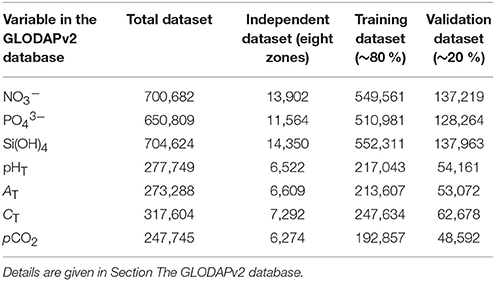
Table 1. Number of data available for each variable in the different datasets used in this study: the general GLODAPv2 database (data that passed the secondary quality control, except for the Mediterranean data), the dataset from the eight independent zones that were first removed from the general database, the dataset used to train the neural network (80 % of the general database minus the eight independent zones), and the dataset used to validate the neural network (20 %).

Neural Network Development

General Principle of Multi-Layered Perceptron (MLP)

A multi-layer perceptron (MLP; Bishop, 1995; Rumelhart et al., 1988) is an artificial neural network based on several layers (i.e., the so-called input, hidden, and output layers) composed of neurons which are basically elementary transfer functions. These neurons are interconnected with the neurons of the preceding and following layers by weights (Figure 2), which are iteratively readjusted during the training phase of the MLP. The criterion for readjusting the weights is the minimization of a cost function defined as the quadratic difference between the reference measurements and the MLP-based outputs. This minimization is done through the back-propagation conjugate-gradient technique (Hornik et al., 1989; Bishop, 1995), an iterative optimization method adapted to the development of MLPs. To prevent overlearning (Bishop, 1995), the training data set is randomly split into two subsets called “learning” and “test” data sets (50 % of the training dataset each). Finally the validation data set is used to evaluate the final method performance. Moreover, the “independent data set” (see above in Section The GLODAPv2 Database) is used to check the general applicability of the method.

FIGURE 2

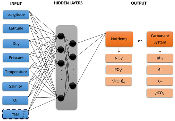
Figure 2. Schematic representation of the CANYON MLP-based neural-network algorithm that retrieves the concentrations of nutrients [NO₃⁻, PO₄³⁻, and Si(OH)₄] and the parameters of the carbonate system in seawater (pH_T, A_T, C_T, and pCO₂). The input variables are field measured temperature, salinity, O₂, and hydrostatic pressure (i.e., depth) together with the geolocation and time of sampling. The year is used as input only for retrieving pH_T, C_T, and pCO₂. Doy, day of year.

CANYON: Developing a MLP to Retrieve Nutrient and Carbonate System Concentrations

The optimal architectures of CANYON MLPs for the seven variables to retrieve (i.e., concentrations of three dissolved macronutrients, NO₃⁻, PO₄³⁻, Si(OH)₄, and four parameters of the carbonate system, pH_T, A_T, C_T, and pCO₂) were chosen after multiple tests. As summarized in Figure 2, the chosen input variables include hydrological and biogeochemical components (i.e., temperature, salinity, and O₂ measurements), spatial components (i.e., hydrostatic pressure, latitude, and longitude) and a temporal component (i.e., day of the year, doy, for the seven variables, and the year for only pH_T, C_T, and pCO₂ retrievals). We chose to use the year as input of the MLPs developed for retrieving pH_T, C_T, and pCO₂ in order to take into account the long-term changes in seawater CO₂-carbonate chemistry due to the uptake of anthropogenic CO₂ (e.g., Gattuso and Hansson, 2011).

Prior to the full-depth CANYON version in this study, an initial depth-restricted CANYON algorithm (i.e., 30 – 1,500 dbar depth range) was first developed, and showed a very good performance in subsurface, mode, and intermediate waters. However, estimated concentrations at 1,500 dbar occasionally showed small-amplitude seasonal cycles (data not shown). This especially occurred in regions with scarce reference data, where spatially adjacent data had been acquired in different seasons. We believe that, when the day of the year (doy) had been provided as extra degree of freedom at depth to the MLP, per-se spatial variability was parameterized as seasonal variability. To avoid this misattribution by the neural network, we decided to develop the full-depth CANYON where the doy information is not provided below a certain depth. This depth is the larger of 750 dbar or the climatological maximum mixed layer depth (Holte et al., 2016), below which no seasonal cycle is expected.

For the full-depth CANYON algorithm development, the pressure input was specifically transformed by a combination of a linear and a logistic curve according to:

$\text{P}=\frac{\text{P}}{20000 \text{dbar}}+\frac{1}{{\left(1+\text{exp}\left(-\frac{\text{P}}{300 \text{dbar}}\right)\right)}^3}$

for two main reasons. (1) Based on our previous experience of including doy in the model, we wanted to limit the degrees of freedom of the neural network in deep and abyssal waters and focus instead its parameterization on temperature and salinity, i.e., the water mass properties. Preliminary analysis confirmed that temperature and salinity were the main determinants of nutrient concentrations and carbonate system parameters in the deep water masses. (2) Preliminary analysis showed that sub-surface and mode-water CANYON estimates for a full-depth version without pressure transformation were less satisfactory than our initial 30 – 1,500 dbar version. We attributed this to the extension of the pressure range to full ocean depth, where sub-surface, and mode waters comprise a much smaller dynamic range than previously. To counteract this effect, we chose the above input transformation of pressure with the aim to mimic the dynamic range of our initial CANYON in the interval between 0 and 1,000 dbar.

The uncertainty of the pCO₂ calculation from C_T and A_T is proportional to pCO₂, i.e., high pCO₂ levels have a higher uncertainty than low pCO₂ levels. Similarly, the uncertainty of the CANYON-predicted pCO₂ scales with pCO₂ as well. The cost function of the MLP training (the quadratic difference between reference and MLP output), however, works on the absolute pCO₂-value. To account for the different behavior of pCO₂ and to avoid potential biases to the MLP induced by large absolute pCO₂-values (with large uncertainties) during training, we transformed the pCO₂ to a hypothetical, pCO₂-equivalent C_T at constant conditions (i.e., A_T 2,300 μmol kg⁻¹, 25 °C, 35 salinity, 0 dbar, zero silicate and phosphate) before training. A constant change in this hypothetical C_T corresponds to a change in pCO₂ that is proportional to pCO₂. This transformation thus approximates the observed pCO₂ behavior while we retain the benefits of our MLP architecture and the backpropagation technique for training.

Similarly to the methods developed by Sauzède et al. (2015, 2016), a specific normalization procedure was applied to the doy and longitude inputs to take into account the periodicity of these variables (e.g., doy 1 of a given year is very similar from a seasonal perspective to doy 365 of the previous year). These two input variables were transformed into radians:

${\text{X}}_{\text{rad}}=\frac{\text{X}.\pi }{\text{a}}$

where X was either the doy or the longitude, and a was a constant equal to 182.625 or 180 for the doy or the longitude, respectively (accounting for half the number of days in the year and half the maximum value of longitude, respectively). Moreover, as the elementary transfer function that provided outputs when inputs were applied to the MLP was a sigmoid non-linear function and subsequently varied within the [−1;1] domain, the inputs and outputs of the MLP were centered and reduced to match the range [−1;1] (see details in Sauzède et al., 2016).

Finally, the MLP developed in this study for each of the seven variables to retrieve (i.e., output variables) are composed of the input layer, two hidden layers, and one output layer (schematic overview in Figure 2). To choose the best architecture of each MLP, tests were performed using one or two hidden layers with a number of neurons varying between 1 and 50 and 1 and 20, respectively. The MLP architecture for each output variable with minimum error of validation and minimum number of neurons was then selected as the best (Table 2). In order to evaluate the method robustness for each MLP, several subsets of the training data set were tested with no difference observed in the prediction.

TABLE 2

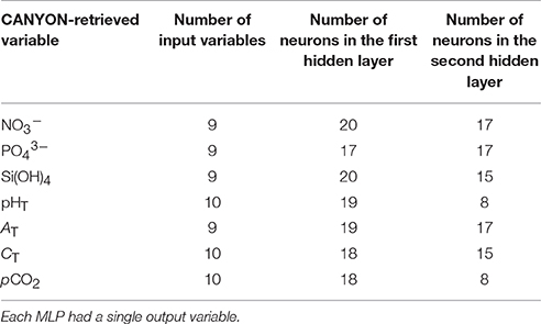
Table 2. Characteristics of the Multi-Layered Perceptron architecture for each CANYON-retrieved variable.

Statistical Evaluation of Method Performance

Four statistics were chosen to evaluate the CANYON algorithms performance on the validation datasets. The coefficient of determination (r²) and the slope of the linear regression between the CANYON-retrieved values and the corresponding GLODAPv2 measurements were computed. The statistics also included the MAE (Mean Absolute Error) and the RMSE (Root Mean Squared Error) to evaluate the errors and accuracies of each model:

$\begin{array}{l}\text{MAE}=\frac{1}{\text{N}}.{\displaystyle \sum _{\text{i}=1}^{\text{N}}|{\text{X}}_{\text{CANYON} \text{i}}-{\text{X}}_{\text{GLODAPv}2 \text{i}}|}\\ \text{RMSE}=\sqrt{\frac{1}{\text{N}}.{\displaystyle \sum _{\text{i}=1}^{\text{N}}{\left({\text{X}}_{\text{CANYON} \text{ i}}-{\text{X}}_{\text{GLODAPv}2 \text{i}}\right)}^2}}\end{array}$

Note that absolute uncertainties are expressed as values for NO₃⁻, PO₄³⁻, Si(OH)₄, pH_T, A_T, and C_T parameters_. For pCO₂ parameter, the relative uncertainties are expressed as percentages (e.g., a relative uncertainty of 5 % is an absolute uncertainty of 20 μatm at 400 μatm).

Results and Discussion

Overall CANYON Performance

Using the validation database (i.e., 20 % of the general database minus the eight independent zones), we evaluated the performance of the method by comparing the CANYON-retrieved nutrient concentrations and carbonate system parameters with the measurements in the GLODAPv2 database using the statistics from Section Statistical Evaluation of Method Performance. Scatterplots of CANYON-retrieved variables vs. GLODAPv2 measurements (Figure 3) show that the CANYON method predicts nutrient concentration and carbonate system parameters with good accuracy (i.e., of 0.93, 0.066, and 3.0 μmol kg⁻¹ for the concentrations of NO₃⁻, PO₄³⁻, and Si(OH)₄, respectively, and of 0.019, 7 μmol kg⁻¹, 10 μmol kg⁻¹ and 5.1 % or 20 μatm at 400 μatm for pH_T, A_T, C_T, and pCO₂, respectively). The determination coefficients of the seven linear models between the CANYON-retrieved and GLODAPv2-variables are comprised between 0.982 and 0.996 with slopes ranging from 0.986 to 0.999. In Figure 3 only very few data points diverge from the 1:1 line. A higher scatter is observed for low CANYON-retrieved NO₃⁻ (and PO₄³⁻), which mostly corresponds to low surface nutrient concentrations inside and at the edges of the subtropical gyres. Moreover, the higher scatter observed near the surface than deeper for most variables is probably due to the higher inherent variability in the surface.

FIGURE 3

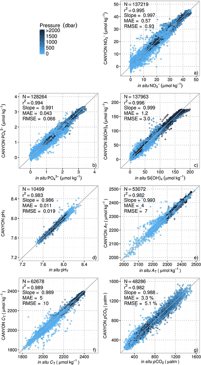
Figure 3. Comparison of the values retrieved by CANYON with the corresponding measurements in the GLODAPv2 database for: (a) NO₃⁻; (b) PO₄³⁻; (c) Si(OH)₄; (d) pH_T; (e) A_T; (f) C_T; and (g) pCO₂ with data ordered according to the pressure. The 1:1 line is shown in each plot as visual reference. The statistics are defined in Section Statistical Evaluation of Method Performance.

To go further, the final CANYON-accuracies for the seven variables can be estimated using the merged accuracies of CANYON estimations and GLODAPv2 measurements (RMSE_final = √[RMSE_CANYON² + RMSE_{RMSEGLODAPv2²}]). The accuracies of GLODAPv2 measurements are 0.46, 0.033, and 1.1 μmol kg⁻¹, for NO₃⁻, PO₄³⁻, Si(OH)₄, respectively, and 0.005, 6 μmol kg⁻¹, and 4 μmol kg⁻¹, for pH_T, A_T, and C_T, respectively from Olsen et al. (2016) and 5.6 % (22 μatm at 400 μatm) for pCO₂ from uncertainty propagation of the carbonate system calculations using seacarb errors (Gattuso et al., 2015, 2016). Thus, ultimately, the final global accuracies of CANYON are 1.04, 0.074, and 3.2 μmol kg⁻¹ for NO₃⁻, PO₄³⁻, and Si(OH)₄ concentrations, respectively, and 0.020, 9 μmol kg⁻¹, 11 μmol kg⁻¹ and 7.6 % (30 μatm at 400 μatm) for pH_T, A_T, C_T, and pCO₂, respectively.

The training and validation datasets of the neural networks used to retrieve carbonate system parameters were smaller than the datasets for the retrieval of nutrient concentrations (Figure 3 and Table 1). It is thus possible that the carbonate system networks are less robust than the nutrient ones. In any case, all the MLPs could be updated in the future as more data become available; this seems especially important for the pH_T database, which is presently the least populated. In order to assess the importance of this potential weakness, we developed a special neural network using all pH_T data available, i.e., all the data that passed the primary quality control (see details in Section The GLODAPv2 Database). The results of this special CANYON algorithm, based on more but a priori less accurate data used for training, are not improved when compared to our initial results (i.e., RMSE of 0.030). Given this and in order to maintain consistency among CANYON algorithms and their retrieval performance, all neural networks were trained using data that had passed the secondary quality control (except for the Mediterranean Sea, see details in Section The GLODAPv2 Database).

To identify possible trends, errors were plotted against each input variable for each retrieved nutrient concentration (Figure 4) and carbonate system parameter (Figure 5). Some errors are larger because of the small numbers of data (the intensity of the shading in each box refers to the number of data). Nevertheless, some clear trends are observed. The range of errors for Si(OH)₄ retrieval seems to be higher at high latitudes in the Southern hemisphere (i.e., latitudes <−60°) and low temperatures, i.e., the ranges of box-plot whiskers increased with both decreasing latitude and temperature in Figure 4. This corresponds to regions of significant Si(OH)₄, mostly in the Southern Ocean, which suggests that the CANYON method is less accurate for Si(OH)₄ retrievals in the Southern Ocean than in other areas. The C_T estimates show a high error at high temperatures and unusually low (<34 psu) salinities. pCO₂ estimates exhibit an increased uncertainty at the extremes of the O₂ input (Figure 5), i.e., the range of errors increases at low O₂ concentrations corresponding to high pCO₂ (Figure S3), and at high O₂ concentrations corresponding to cold, low salinity polar surface waters. For CANYON-estimated NO₃⁻, PO₄³⁻, and C_T, the upper layer (i.e., ≤700 m) has the broadest error range. The Si(OH)₄ displays an opposite trend with error larger for deeper than surface waters (i.e., ≥700 m). The CANYON-estimated A_T, pH_T, and pCO₂ errors are not affected by depth inputs. Finally, Figure S3 shows that the CANYON retrieved variables are not biased against the range of in situ values to retrieve, except for a few extreme values where few data (i.e., lightly shaded boxes) were available in the training and validation databases.

FIGURE 4

Figure 4. Box plots of the differences between CANYON estimates minus GLODAPv2 reference measurements for (from left to right): NO₃⁻ (μmol kg⁻¹), PO₄³⁻(μmol kg⁻¹), and Si(OH)₄ (μmol kg⁻¹) vs. the variable indicated on the left: pressure (P), year, doy, longitude, latitude, temperature (T), salinity (S), O₂. The intensity of the shading in each box refers to the number of data. The intervals were created by dividing the range of values in eight equal intervals. For each box, the negative and positive whiskers represent the Q1–1.5*IQR and Q3 + 1.5*IQR, respectively, where Q1 is the 0.25 quantile, Q3 the 0.75 quantile, and IQR the inter-quantile range. The width of each box represents the IQR and the middle line the median of the values.

FIGURE 5

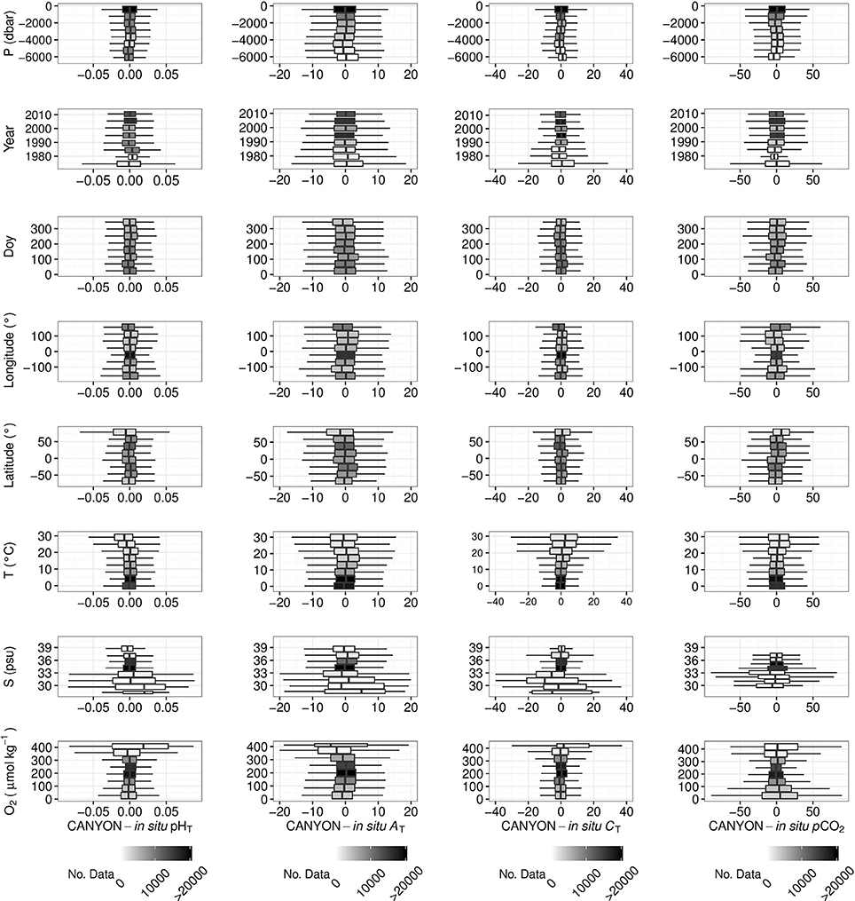
Figure 5. Box plots of the difference between CANYON estimates minus GLODAPv2 reference measurements for (from left to right) pH_T, A_T (μmol kg⁻¹), C_T (μmol kg⁻¹), and pCO₂ (μatm) vs. the variable indicated on the left: pressure (P), year, doy, longitude, latitude, temperature (T), salinity (S), O₂. The intensity of the shading in each box refers to the number of data. The intervals were created by sharing the range of values in eight regular intervals. For each box, the lower and upper whiskers represent the Q1–1.5*IQR and Q3+1.5*IQR, respectively, with Q1 the 0.25 quantile, Q3 the 0.75 quantile and IQR the inter-quantile range. The width of each box represents the IQR and the middle line the median of the values.

The above results indicate that hydrographic data and information about season (doy) and geolocation can certainly predict some aspects of the dynamics of biogeochemical variables at the surface (e.g., nutrient and C_T drawdown during the spring bloom, seasonal reset to preformed nutrient concentrations with winter ventilation) with O₂ being the most important predictor in CANYON for production and remineralization, particularly in the ocean interior. The year is the only variable that accounts in CANYON for the increase in anthropogenic CO₂. As a consequence, when the year was not included, CANYON-estimated pH_T, C_T, and pCO₂ showed a clear remaining trend due to the missing information about the long-term changes in seawater CO₂-carbonate chemistry (data not shown).

Independent Validation for Eight Geographic Zones

The smoothed mean differences between CANYON-retrieved and in situ measurements were plotted as vertical profiles for each of the seven variables and the eight independent zones (Figure 6). In general, the accuracy (i.e., RMSE) for each variable is comparable to the accuracy determined on the validation data set (Table 3). Beyond this general agreement, there are a few discrepancies. The errors appear to be higher in the 0 – 200 m layer than below. This is maybe due to a larger variability in this upper layer, caused by not only biogeochemical processes but also air-sea exchange of O₂ that act to decouple O₂ from the CANYON outputs (see also Figure 3). The Sub-Equatorial Pacific, North Pacific and South Atlantic display higher RMSE than calculated from the 20 % validation data (Table 3). These results suggest that the GLODAPv2 data set for these specific zones could have been underrepresented in the training database with respect to the regional variability in nutrient concentrations and carbonate system parameters.

FIGURE 6

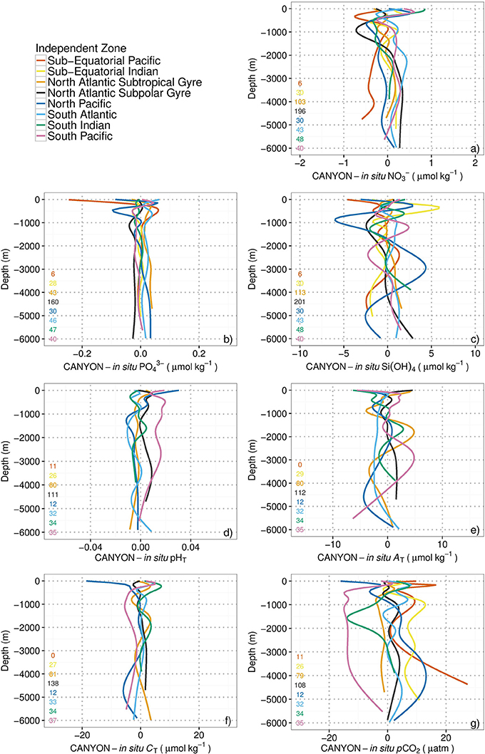
Figure 6. Vertical profiles of the smoothed mean differences between CANYON-retrieved and in situ measurements from surface to 6,000 m depth for: (a) NO₃⁻; (b) PO₄³⁻; (c) Si(OH)₄; (d) pH_T; (e) A_T; (f) C_T; and (g) pCO₂. The number of profiles used to compute the mean difference for each zone is indicated in the bottom left-hand side of each panel. Color code: eight independent zones in Figure 1.

TABLE 3

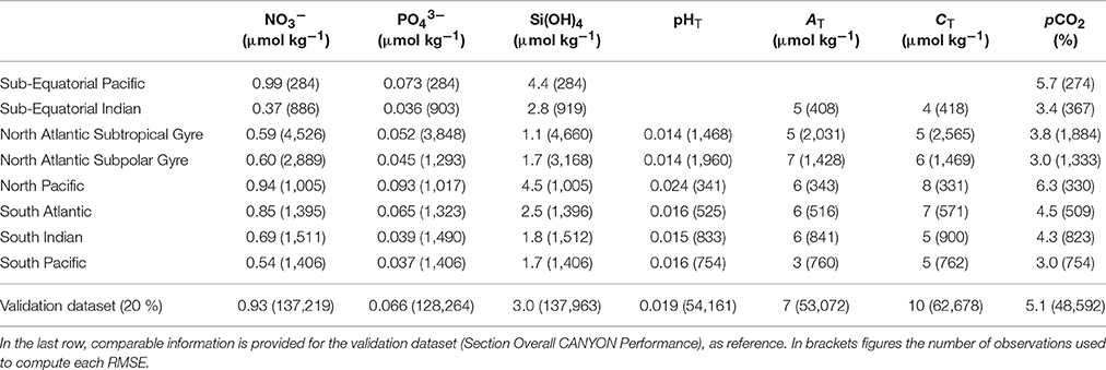
Table 3. CANYON retrieval accuracy (RMSE) for each variable in each of the eight independent zones.

The above comparisons and the identification of spatio-temporal domains where CANYON performed less accurately could be used to identify more objectively the periods or regions that require more intense acquisition of discrete high-quality measurements. Indeed, the periods and regions where CANYON fails to reproduce well in situ observations are those where the variability (mostly seasonal) was not well-represented in the training dataset. From Table 3 and Figure 6, these regions are mainly the Sub-Equatorial Pacific, the North Pacific and the South Atlantic, and the periods are most likely late autumn and winter, when harsh sea conditions generally prevent ship-based collection of high-quality measurements. In fact, the GLODAPv2 database seems to be biased in this respect (Section The GLODAPv2 Database and Figure S2).

Further Results for Specific Applications

Here we present further results important for specific applications. Indeed, one of a potential application of the CANYON method is the calibration of NO₃⁻ and pH_T sensors mounted on BGC-Argo profiling floats (because the corresponding sensors may drift over long-term deployment). To overcome this problem, CANYON could be used to compute deep (e.g., ≥1,000 m) reference measurements each time the float profiles. With this aim in mind, specific MLPs were developed to retrieve NO₃⁻ concentration and pH_T only at depths between 950 and 2,050 m, i.e., different from the full water-column MLPs used above. Results show that specific, deep MLPs do not significantly improve the quality of the results compared to the MLPs developed for the entire water column applied to this layer (i.e., RMSE for NO₃⁻ of 0.50 and 0.54 μmol kg⁻¹, respectively, and for pH_T of 0.013 units for the two approaches). The CANYON method can therefore be used to retrieve NO₃⁻ concentration and pH_T for specific applications focused on deep layers with excellent accuracy.

For pCO₂ applications, most studies focus on the surface layer of the open ocean and on CO₂ air-sea exchange (e.g., Takahashi et al., 2009). The CANYON method could be used to address the regional and seasonal variability of air-sea CO₂ fluxes in view of comparing it with the results of previous studies based on neural networks (Landschützer et al., 2014, 2016). For this application, it is important to ascertain that the general MLP performs as adequately as a specific MLP developed to retrieve pCO₂ for the surface layer only (i.e., ≤100 m). Here again, the CANYON algorithm developed for the entire water column is as robust as a specific, surface-focused MLP (i.e., RMSE of 34 and 33 μatm, respectively).

Example of Application: Illustration with HOT Database

The CANYON method was further applied outside the GLODAPv2 domain, on which it was trained, using an independent dataset that contained similar variables. The Hawaii Ocean Time Series (HOT) database contains monthly vertical profiles of hydrological properties, O₂, nutrient concentrations and carbonate system parameters from the deep-water station ALOHA since 1994 (Karl and Lukas, 1996; Dore et al., 2003). The HOT temperature, salinity, and O₂ measurements from HOT were used as input variables to estimate the concentrations of nutrients and the carbonate system parameters. The overall agreement between the CANYON-simulated variables and their measured in situ counterparts is satisfactory, as shown by the absolute differences between the two datasets and the corresponding comparison statistics (Figure 7 and Table 4). There are few systematic biases, such as the model underestimation of NO₃⁻ from 450 to 550 m (i.e., the depth horizon of the nitracline) and the overestimation of PO₄³⁻ and C_T in the upper 150 m (Figures 7b,d,l, respectively).

FIGURE 7

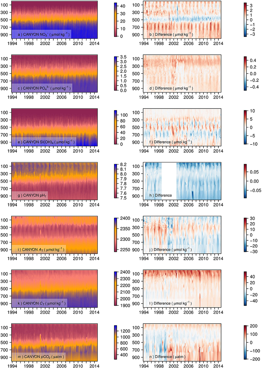
Figure 7. Values predicted by CANYON (a,c,e,g,i,k,m) and absolute differences between HOT measurements and CANYON estimates (b,d,f,h,j,l,n). Time series (22 years) for NO₃⁻ (a,b), PO₄³⁻ (c,d), Si(OH)₄ (e,f), pH_T (g,h), A_T (i,j), C_T (k,l), and pCO₂ (m,n). Five profiles from 25 February 2003 to 29 March 2003 have been removed from the time-series because of their abnormal O₂ profiles (see details in Section Example of Application: Illustration with HOT Database).

TABLE 4

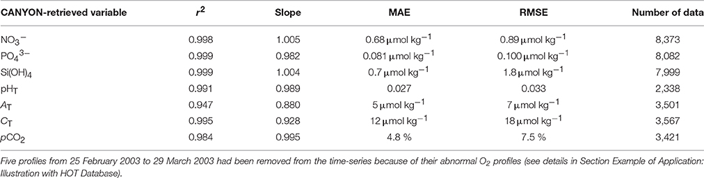
Table 4. Comparison statistics between the values retrieved by CANYON vs. the corresponding measurements in the HOT database.

Interestingly, running CANYON on this dataset unraveled O₂ outliers in the database. A first run of CANYON produced abnormally high differences between the retrieved and in situ values of the seven CANYON-estimated variables for profiles from 25 February 2003 to 29 March 2003. This corresponded to five O₂ profiles with abnormally high concentrations of O₂ (see black triangles in Figure S4). These profiles were subsequently removed from the analysis to avoid contaminating the CANYON-retrieved data shown in Figure 7 and the corresponding statistics in Table 4.

CANYON also provided a way to fill a gap in the HOT dataset. Indeed, pH_T had not been acquired during the 1999–2003 period, but the input variables needed to run CANYON had been measured. pH_T could thus be estimated during that period (Figure 7g) with a mean accuracy of 0.033 units (i.e., RMSE in Table 4). However, it is obviously not possible to compare the values predicted by CANYON with (non-existent) corresponding in situ measurements from 1999 to 2003 (Figure 7h).

Using the HOT temperature, salinity and O₂ measurements from the last year, i.e., 2015, we estimated pH_T for the 15 years to come (by changing only the year input in CANYON), and a decline is found in pH_T of 0.024 units over this 15-year period (i.e., decrease of 0.0016 ± 0.0004 units year⁻¹). This value is consistent with the decrease in pH_T of 0.0019 ± 0.0002 year⁻¹ reported in the central North Pacific (Dore et al., 2009) and more generally of 0.0013 to 0.0026 units year⁻¹ units during the 20–30 last years (Bates et al., 2014). This suggests that the CANYON approach could perhaps also be used outside the temporal range of training for the carbonate system parameters for estimating near future changes in pH_T, C_T, and pCO₂, thanks to the use of the year among the input variables. However, this would assume that the relationships between the input and output variables, through the hidden layers of the CANYON model, will remain unchanged in the future, and the sensitivity of retrieved carbonate system parameters to departures from this assumption remains to be explored.

Conclusions and Perspectives

The global Biogeochemical-Argo (BGC-Argo) program is being progressively implemented (Johnson and Claustre, 2016), and its core variables include O₂. BGC-Argo floats can now acquire high-quality vertical profiles of O₂ on the long term (Bittig and Körtzinger, 2015; Johnson et al., 2015; Bushinsky et al., 2016). Given the possibility of acquiring long-term, global vertical profiles of temperature, salinity and O₂, CANYON could be used to develop a variety of new applications.

Firstly, CANYON may contribute to developing quality control and post-processing procedures for NO₃⁻ concentration and pH_T in oceanic waters (see Section Further Results for Specific Applications). These two variables, together with O₂, are core BGC-Argo variables and their measurements make use of an optical sensor for NO₃⁻ (Johnson and Coletti, 2002) and an electrochemical sensor for pH_T (Johnson et al., 2016) with known accuracies (1 μM and 0.010 for NO₃⁻ and pH_T, respectively; Johnson et al., 2013, 2016). However, these sensors, like the O₂ probes, drift over long-term deployments. Following an approach similar to the one developed for oxygen sensors, which can be referenced to atmospheric values each time the floats surface (Bittig and Körtzinger, 2015; Johnson et al., 2015; Bushinsky et al., 2016), CANYON could be used to compute deep (e.g., ≥1,000 m) reference measurements at depth for pH_T and NO₃⁻ each time the float makes a profile. At these depths, it is indeed expected that reliable and stable reference measurements could be acquired, which could be used to develop appropriate correction procedures for NO₃⁻ concentration and pH_T and thus guarantee the long-term accuracy of the sensors.

Secondly, CANYON can also provide estimates, with known accuracies, of variables that are not presently measured by BGC-Argo floats. This is the case for PO₄³⁻ and Si(OH)₄ and the three other variables of the carbonate system than pH_T. CANYON could thus be used as a cost-effective method for “filling the spatio-temporal gaps” of these variables by populating spatially and temporally their loosely resolved fields in oceanic waters. For these under-sampled variables, CANYON offers novel opportunities at global and local scales. For example, global fields of these variables provided by CANYON could support the initialization and validation of biogeochemical models which presently crucially lack reference data (e.g., Doney et al., 2009; Ilyina et al., 2013).

Thirdly, CANYON could also be used in combination with present measurements of the respective field nutrient concentrations and/or carbonate system parameters. Beside quality control of these data, CANYON values could serve to identify unusual biogeochemical events that had not been covered by the global but sparse GLODAPv2 training data set, in cases where CANYON and field data diverge.

Fourthly, and for more local approaches (e.g., analysis of individual float time series), the possible derivation of pCO₂ from BGC-Argo float O₂ and ancillary measurements (with or without pH_T) potentially represents a new way to address regional and seasonal variability in CO₂ air-sea exchanges, and to reduce present uncertainties in the estimates of these fluxes. Moreover, estimating the three macronutrients (NO₃⁻, PO₄³⁻, and Si(OH)₄) from BGC-Argo float data could be of great value for better understanding the dynamics of biogeochemical events such as the development and subsequent collapse of phytoplankton blooms.

Fifthly, CANYON could contribute to design future observational programs by identifying areas and periods where data acquisition could most cost-effectively address variability that is presently unresolved. Indeed, the strict quality control of the input data in the present study (which used only GLODAPv2 data that passed the second quality check, see Section The GLODAPv2 Database) eliminated some specific regions from our training and validation datasets. This argues for developing field-based observation programs to conduct high-quality measurements in these areas. More generally, the spatio-temporal domains where CANYON provided the least satisfactory results likely corresponded to weaknesses in the GLODAPv2 database with respect to catching the inherent and natural variability of different variables, such as the Southern Ocean in winter.

Overall, the CANYON-type estimation of biogeochemical variables based on data provided by the global BGC-Argo program offers new avenues for marine biogeochemistry that are comparable to those that have been created for physical oceanography by the Argo network since the early 2000s. This novel approach could increase tremendously the value of biogeochemical measurements made on board ships and by BGC-Argo floats by combining the high quality of the first type of data with the broad spatio-temporal coverage of the second.

Author Contributions

HC, RS, and OP have initiated the study and designed the neural-network configurations with JG and HB. RS ran simulations and created the plots. All authors contributed to analysis and discussion of results. RS wrote most part of the manuscript. All authors commented on and contributed to the improvement of several versions of the manuscript.

Conflict of Interest Statement

The authors declare that the research was conducted in the absence of any commercial or financial relationships that could be construed as a potential conflict of interest.

Acknowledgments

This study was supported by the remOcean project (funded by the European Research Council, Grant Agreement No. 246777) and the AtlantOS project (funded by the European Union's Horizon 2020 research and innovation program, Grant Agreement No. 2014-633211). This is a contribution to the Southern Ocean Carbon and Climate Observations and Modeling (SOCCOM) project which is supported by the US National Science Foundation (PLR-1425989). We want to thank Tobias Steinhoff (GEOMAR, Kiel), for helpful discussions on carbonate system calculations. We deeply acknowledge the work from analysts, investigators, and crew who collected the data at sea. We are also grateful to all who have contributed their data to GLODAPv2 project and acknowledge the huge effort made to gather all data to create the GLODAPv2 database.

Supplementary Material

The Supplementary Material for this article can be found online at: https://www.frontiersin.org/article/10.3389/fmars.2017.00128/full#supplementary-material

Figure S1. Geographic boundaries of the seven major oceanic basins used in Section The GLODAPv2 Database.

Figure S2. Temporal distribution of the number of observations (N_obs) available in GLODAPv2 that were used to develop CANYON MLPs, plotted as a function of the sampling months (top) and years (bottom). The colors refer to the sampling latitude: North high latitudes (≥45°); North mid latitudes (≥15° and <45°); Equatorial latitudes (>−15° and <15°); South mid latitudes (>–45° and ≤−15°), and South high latitudes (≤−45°).

Figure S3. Box plots of the difference between CANYON estimates minus GLODAPv2 reference measurements for the seven variables: NO₃⁻ (μmol kg⁻¹), PO₄³⁻ (μmol kg⁻¹), Si(OH)₄ (μmol kg⁻¹), pH_T, A_T (μmol kg⁻¹), C_T (μmol kg⁻¹), and pCO₂ (μatm) vs. the range of the variable retrieved (output variable). The intensity of the shading in each box refers to the number of data. The intervals were created by sharing the range of values in eight regular intervals. For each box, the lower and upper whiskers represent the Q1–1.5*IQR and Q3+1.5*IQR, respectively, with Q1 the 0.25 quantile, Q3 the 0.75 quantile, and IQR the inter-quantile range. The width of each box represents the IQR and the middle line the median of the values.

Figure S4. Time series (22 years) of the temperature (a), the salinity (b), and the O₂ (c) measured at HOT. The five profiles from 25 February 2003 to 29 March 2003 that had been removed from the time-series because of their abnormal O₂ profiles are shown with the black triangle in the panel (c)—(see details in Section Example of Application: Illustration with HOT Database).

References

Bates, N., Astor, Y., Church, M., Currie, K., Dore, J., Gonaález-Dávila, M., et al. (2014). A time-series view of changing ocean chemistry due to ocean uptake of Anthropogenic CO2 and ocean acidification. Oceanography 27, 126–141. doi: 10.5670/oceanog.2014.16

CrossRef Full Text | Google Scholar

Ben Mustapha, Z., Alvain, S., Jamet, C., Loisel, H., and Dessailly, D. (2013). Automatic classification of water-leaving radiance anomalies from global SeaWiFS imagery: application to the detection of phytoplankton groups in open ocean waters. Remote Sens. Environ. 146, 97–112. doi: 10.1016/j.rse.2013.08.046

CrossRef Full Text | Google Scholar

Bishop, C. M. (1995). Neural Networks for Pattern Recognition. Oxford University Press, Inc. Available online at: http://dl.acm.org/citation.cfm?id=525960 (Accessed March 20, 2014).

Google Scholar

Bittig, H. C., and Körtzinger, A. (2015). Tackling oxygen optode drift: near-surface and in-air oxygen optode measurements on a float provide an accurate in situ reference. J. Atmos. Ocean. Technol. 32, 1536–1543. doi: 10.1175/JTECH-D-14-00162.1

CrossRef Full Text | Google Scholar

Bushinsky, S. M., Emerson, S. R., Riser, S. C., and Swift, D. D. (2016). Accurate oxygen measurements on modified Argo floats using in situ air calibrations. Limnol. Oceanogr. Methods 14, 491–505. doi: 10.1002/lom3.10107

CrossRef Full Text | Google Scholar

Carter, B. R., Williams, N. L., Gray, A. R., and Feely, R. A. (2016). Locally interpolated alkalinity regression for global alkalinity estimation. Limnol. Oceanogr. Methods 14, 268–277. doi: 10.1002/lom3.10087

CrossRef Full Text | Google Scholar

Claustre, H., Antoine, D., Boehme, L., Boss, E., D'Ortenzio, F., Fanton D'Andon, O., et al. (2010). “Guidelines towards an integrated ocean observation system for ecosystems and biogeochemical cycles,” in Proceedings of OceanObs'09: Sustained Ocean Observations and Information for Society, eds J. Hall, D. E. Harrison, and D. Stammer (Venice: European Space Agency), 546–566.

Google Scholar

Dickson, A. G. (1990). Standard potential of the reaction AGCL(S)+1/2H-2(G) = AG(S)+HCL(AQ) and the standard acidity constant of the ion HSO4− in synthetic sea water from 273.15 to 318.15 K. J. Chem. Thermodyn. 22, 113–127. doi: 10.1016/0021-9614(90)90074-Z

CrossRef Full Text | Google Scholar

Doney, S. C., Fabry, V. J., Feely, R. A., and Kleypas, J. A. (2009). Ocean acidification: the other CO₂ problem. Ann. Rev. Mar. Sci. 1, 169–192. doi: 10.1146/annurev.marine.010908.163834

PubMed Abstract | CrossRef Full Text | Google Scholar

Dore, J. E., Lukas, R., Sadler, D. W., and Karl, D. M. (2003). Climate-driven changes to the atmospheric CO2 sink in the subtropical North Pacific Ocean. Nature 424, 754–757. doi: 10.1038/nature01885

PubMed Abstract | CrossRef Full Text | Google Scholar

Dore, J. E., Lukas, R., Sadler, D. W., Church, M. J., and Karl, D. M. (2009). Physical and biogeochemical modulation of ocean acidification in the central North Pacific. Proc. Natl. Acad. Sci. U.S.A. 106, 12235–12240. doi: 10.1073/pnas.0906044106

PubMed Abstract | CrossRef Full Text | Google Scholar

Friedrich, T., and Oschlies, A. (2009). Neural network-based estimates of North Atlantic surface pCO₂ from satellite data: a methodological study. J. Geophys. Res. 114, C03020. doi: 10.1029/2007JC004646

CrossRef Full Text | Google Scholar

Gattuso, J.-P., and Hansson, L. (2011). Ocean Acidification. Oxford: Oxford University Press.

Google Scholar

Gattuso, J.-P., Epitalon, J.-M., and Lavigne, H. (2016). Seacarb: Seawater Carbonate Chemistry R Package Version 3.0.14. Available online at: https://cran.r-project.org/package=seacarb

Gattuso, J.-P., Magnan, A., Bille, R., Cheung, W. W. L., Howes, E. L., Joos, F., et al. (2015). Contrasting futures for ocean and society from different anthropogenic CO2 emissions scenarios. Science 349, aac4722–aac4722. doi: 10.1126/science.aac4722

CrossRef Full Text | Google Scholar

Gouretski, V., and Jancke, K. (2000). Systematic errors as the cause for an apparent deep water property variability: global analysis of the WOCE and historical hydrographic data. Prog. Oceanogr. 48, 337–402. doi: 10.1016/S0079-6611(00)00049-5

CrossRef Full Text | Google Scholar

Gruber, N. (2011). Warming up, turning sour, losing breath: ocean biogeochemistry under global change. Philos. Trans. A Math. Phys. Eng. Sci. 369, 1980–1996. doi: 10.1098/rsta.2011.0003

PubMed Abstract | CrossRef Full Text | Google Scholar

Gruber, N., Doney, S. C., Emerson, S., Gilbert, D., Kobayashi, T., Kortzinger, A., et al. (2010a). “Adding oxygen to argo: developing a global in situ observatory for ocean deoxygenation and biogeochemistry,” in Proceedings of the “OceanObs'09: Sustained Ocean Observations and Information for Society” Conference, eds J. Hall, D. E. Harrison, and D. Stammer (Venice: ESA publication WPP-306), 432–441 (Accessed September 21–25, 2009). doi: 10.5270/OceanObs09.cwp.39

CrossRef Full Text | Google Scholar

Gruber, N., Körtzinger, A., Borges, A., Claustre, H., Doney, S. C., Feely, R. A., et al. (2010b). “Towards an integrated observing system for ocean carbon and biogeochemistry at a time of change,” in Proceedings of the “OceanObs'09: Sustained Ocean Observations and Information for Society” Conference, eds J. Hall, D. E. Harrison, and D. Stammer (Venice: ESA publication WPP-306) (Accessed September 21–25, 2009). doi: 10.5270/OceanObs09.pp.18

CrossRef Full Text | Google Scholar

Holte, J., Gilson, J., Talley, L., and Roemmich, D. (2016). Argo Mixed Layers, Scripps Institution of Oceanography/UCSD. Available online at: http://mixedlayer.ucsd.edu

Hornik, K., Stinchcombe, M., and White, H. (1989). Multilayer feedforward networks are universal approximators. Neural Netw. 2, 359–366. doi: 10.1016/0893-6080(89)90020-8

CrossRef Full Text | Google Scholar

Ilyina, T., Six, K. D., Segschneider, J., Maier-Reimer, E., Li, H., and Núñez-Riboni, I. (2013). Global ocean biogeochemistry model HAMOCC: model architecture and performance as component of the MPI-Earth system model in different CMIP5 experimental realizations. J. Adv. Model. Earth Syst. 5, 287–315. doi: 10.1029/2012MS000178

CrossRef Full Text | Google Scholar

Jamet, C., Loisel, H., and Dessailly, D. (2012). Retrieval of the spectral diffuse attenuation coefficient K d (λ) in open and coastal ocean waters using a neural network inversion. J. Geophys. Res. 117, C10023. doi: 10.1029/2012JC008076

CrossRef Full Text | Google Scholar

Johnson, G. C., Robbins, P. E., Hufford, G. E., Johnson, G. C., Robbins, P. E., and Hufford, G. E. (2001). Systematic adjustments of hydrographic sections for internal consistency*. J. Atmos. Ocean. Technol. 18, 1234–1244. doi: 10.1175/1520-0426(2001)018<1234:SAOHSF>2.0.CO;2

CrossRef Full Text | Google Scholar

Johnson, K. S., and Claustre, H. (2016). Bringing biogeochemistry into the Argo age. Eos Trans. Am. Geophys. Union 97. doi: 10.1029/2016EO062427. Available online at: https://eos.org/project-updates/bringing-biogeochemistry-into-the-argo-age

CrossRef Full Text | Google Scholar

Johnson, K. S., and Coletti, L. J. (2002). In situ ultraviolet spectrophotometry for high resolution and long-term monitoring of nitrate, bromide and bisulfide in the ocean. Deep Sea Res. Part I Oceanogr. Res. Pap. 49, 1291–1305. doi: 10.1016/S0967-0637(02)00020-1

CrossRef Full Text | Google Scholar

Johnson, K. S., Coletti, L. J., Jannasch, H. W., Sakamoto, C. M., Swift, D. D., and Riser, S. C. (2013). Long-term nitrate measurements in the ocean using the in situ ultraviolet spectrophotometer: sensor integration into the APEX profiling float. J. Atmos. Ocean. Technol. 30, 1854–1866. doi: 10.1175/JTECH-D-12-00221.1

CrossRef Full Text | Google Scholar

Johnson, K. S., Jannasch, H. W., Coletti, L. J., Elrod, V. A., Martz, T. R., Takeshita, Y., et al. (2016). Deep-sea DuraFET: a pressure tolerant ph sensor designed for global sensor networks. Anal. Chem. 88, 3249–3256. doi: 10.1021/acs.analchem.5b04653

PubMed Abstract | CrossRef Full Text | Google Scholar

Johnson, K. S., Plant, J. N., Riser, S. C., and Gilbert, D. (2015). Air oxygen calibration of oxygen optodes on a profiling float array. J. Atmos. Ocean. Technol. 32, 2160–2172. doi: 10.1175/JTECH-D-15-0101.1

CrossRef Full Text | Google Scholar

Johnson, K., Berelson, W., Boss, E., Chase, Z., Claustre, H., Emerson, S., et al. (2009). Observing biogeochemical cycles at global scales with profiling floats and gliders: prospects for a global array. Oceanography 22, 216–225. doi: 10.5670/oceanog.2009.81

CrossRef Full Text | Google Scholar

Juranek, L. W., Feely, R. A., Gilbert, D., Freeland, H., and Miller, L. A. (2011). Real-time estimation of pH and aragonite saturation state from Argo profiling floats: prospects for an autonomous carbon observing strategy. Geophys. Res. Lett. 38, L17603. doi: 10.1029/2011GL048580

CrossRef Full Text | Google Scholar

Karl, D. M., and Lukas, R. (1996). The Hawaii Ocean Time-series (HOT) program: background, rationale and field implementation. Deep Sea Res. Part II Top. Stud. Oceanogr. 43, 129–156. doi: 10.1016/0967-0645(96)00005-7

CrossRef Full Text | Google Scholar

Key, R. M., Olsen, A., Van Heuven, S., Lauvset, S. K., Velo, A., Lin, X., et al. (2015). Global Ocean Data Analysis Project, Version 2 (GLODAPv2). ORNL/CDIAC-162, ND-P093, Carbon Dioxide Information Analysis Center, Oak Ridge National Laboratory, US Department of Energy, Oak Ridge, TN.

Google Scholar

Körtzinger, A., Schimanski, J., Send, U., and Wallace, D. (2004). The ocean takes a deep breath. Science 306, 1337. doi: 10.1126/science.1102557

PubMed Abstract | CrossRef Full Text | Google Scholar

Landschützer, P., Gruber, N., and Bakker, D. C. E. (2016). Decadal variations and trends of the global ocean carbon sink. Global Biogeochem. Cycles 30, 1396–1417. doi: 10.1002/2015GB005359

CrossRef Full Text | Google Scholar

Landschützer, P., Gruber, N., Bakker, D. C. E., and Schuster, U. (2014). Recent variability of the global ocean carbon sink. Global Biogeochem. Cycles 28, 927–949. doi: 10.1002/2014GB004853

CrossRef Full Text | Google Scholar

Landschützer, P., Gruber, N., Bakker, D. C. E., Schuster, U., Nakaoka, S., Payne, M. R., et al. (2013). A neural network-based estimate of the seasonal to inter-annual variability of the Atlantic Ocean carbon sink. Biogeosciences 10, 7793–7815. doi: 10.5194/bg-10-7793-2013

CrossRef Full Text | Google Scholar

Le Quéré, C., Moriarty, R., Andrew, R. M., Canadell, J. G., Sitch, S., Korsbakken, J. I., et al. (2015). Global Carbon Budget 2015. Earth Syst. Sci. Data 7, 349–396. doi: 10.5194/essd-7-349-2015

CrossRef Full Text | Google Scholar

Lek, S., and Guégan, J. F. (1999). Artificial neural networks as a tool in ecological modelling, an introduction. Ecol. Modell. 120, 65–73. doi: 10.1016/S0304-3800(99)00092-7

CrossRef Full Text | Google Scholar

Lueker, T. J., Dickson, A. G., and Keeling, C. D. (2000). Ocean pCO2 calculated from dissolved inorganic carbon, alkalinity, and equations for K1 and K2: validation based on laboratory measurements of CO2 in gas and seawater at equilibrium. Mar. Chem. 70, 105–119. doi: 10.1016/S0304-4203(00)00022-0

CrossRef Full Text | Google Scholar

Martz, T. R., Johnson, K. S., and Riser, S. C. (2008). Ocean metabolism observed with oxygen sensors on profiling floats in the South Pacific. Limnol. Oceanogr. 53, 2094–2111. doi: 10.4319/lo.2008.53.5_part_2.2094

CrossRef Full Text | Google Scholar

Olsen, A., Key, R. M., van Heuven, S., Lauvset, S. K., Velo, A., Lin, X., et al. (2016). The Global Ocean Data Analysis Project version 2 (GLODAPv2) – an internally consistent data product for the world ocean. Earth Syst. Sci. Data 8, 297–323. doi: 10.5194/essd-8-297-2016

CrossRef Full Text | Google Scholar

Perez, F. F., and Fraga, F. (1987). Association constant of fluoride and hydrogen ions in seawater. Mar. Chem. 21, 161–168. doi: 10.1016/0304-4203(87)90036-3

CrossRef Full Text | Google Scholar

Redfield, A. C. (1934). “On the proportions of organic derivatives in sea water and their relation to the composition of plankton,” in James Johnstone Memorial Volume, ed R. J. Daniel (Liverpool: University Press of Liverpool), 176–192.

Redfield, A. C. (1958). The biological control of chemical factors in the environment. Am. Sci. 46, 230A, 205–221.

Google Scholar

Riser, S. C., and Johnson, K. S. (2008). Net production of oxygen in the subtropical ocean. Nature 451, 323–325. doi: 10.1038/nature06441

PubMed Abstract | CrossRef Full Text | Google Scholar

Rumelhart, D. E., Hinton, G. E., and Williams, R. J. (1988). Learning representations by back-propagating errors. Cogn. Model. 5, 696–699.

Google Scholar

Sabine, C. L., Key, R. M., Kozyr, A., Feely, R. A., Wanninkhof, R., Millero, F. J., et al. (2005). Global Ocean Data Analysis Project (GLODAP): Results and Data. Oak Ridge, TN: ORNL/CDIAC-145, NDP-083, Carbon Dioxide Information Analysis Center, Oak Ridge National Laboratory, U.S. Department of Energy, 110.

Sauzède, R., Claustre, H., Jamet, C., Uitz, J., Ras, J., Mignot, A., et al. (2015). Retrieving the vertical distribution of chlorophyll a concentration and phytoplankton community composition from in situ fluorescence profiles: a method based on a neural network with potential for global-scale applications. J. Geophys. Res. Ocean 120, 451–470. doi: 10.1002/2014JC010355

CrossRef Full Text | Google Scholar

Sauzède, R., Claustre, H., Uitz, J., Jamet, C., Dall'Olmo, G., D'Ortenzio, F., et al. (2016). A neural network-based method for merging ocean color and Argo data to extend surface bio-optical properties to depth: retrieval of the particulate backscattering coefficient. J. Geophys. Res. Ocean 121, 2552–2571. doi: 10.1002/2015JC011408

CrossRef Full Text | Google Scholar

Takahashi, T., Sutherland, S. C., Wanninkhof, R., Sweeney, C., Feely, R. A., Chipman, D. W., et al. (2009). Climatological mean and decadal change in surface ocean pCO2, and net sea–air CO2 flux over the global oceans. Deep Sea Res. Part II Top. Stud. Oceanogr. 56, 554–577. doi: 10.1016/j.dsr2.2008.12.009

CrossRef Full Text | Google Scholar

Talley, L. D., Feely, R. A., Sloyan, B. M., Wanninkhof, R., Baringer, M. O., Bullister, J. L., et al. (2016). Changes in ocean heat, carbon content, and ventilation: a review of the first decade of GO-SHIP global repeat hydrography*. Ann. Rev. Mar. Sci. 8, 185–215. doi: 10.1146/annurev-marine-052915-100829

PubMed Abstract | CrossRef Full Text | Google Scholar

Tanhua, T., van Heuven, S., Key, R. M., Velo, A., Olsen, A., and Schirnick, C. (2010). Quality control procedures and methods of the CARINA database. Earth Syst. Sci. Data 2, 35–49. doi: 10.5194/essd-2-35-2010

CrossRef Full Text | Google Scholar

Uppström, L. R. (1974). The boron/chlorinity ratio of deep-sea water from the Pacific Ocean. Deep Sea Res. Oceanogr. Abstr. 21, 161–162. doi: 10.1016/0011-7471(74)90074-6

CrossRef Full Text | Google Scholar

Velo, A., Pérez, F. F., Tanhua, T., Gilcoto, M., Ríos, A. F., and Key, R. M. (2013). Total alkalinity estimation using MLR and neural network techniques. J. Mar. Syst. 111–112, 11–18. doi: 10.1016/j.jmarsys.2012.09.002

CrossRef Full Text | Google Scholar

Ward, B., and Redfern, S. (1999). A neural network model for predicting the bulk-skin temperature difference at the sea surface. Int. J. Remote Sens. 20, 3533–3548. doi: 10.1080/014311699211183

CrossRef Full Text | Google Scholar

Williams, N. L., Juranek, L. W., Johnson, K. S., Feely, R. A., Riser, S. C., Talley, L. D., et al. (2016). Empirical algorithms to estimate water column pH in the Southern Ocean. Geophys. Res. Lett. 43, 3415–3422. doi: 10.1002/2016GL068539

CrossRef Full Text | Google Scholar