Shellfish Aquaculture from Space: Potential of Sentinel2 to Monitor Tide-Driven Changes in Turbidity, Chlorophyll Concentration and Oyster Physiological Response at the Scale of an Oyster Farm

Introduction

One of the most striking features of the intertidal zone is the formation of microphytobenthos (MPB) biofilms at sediment surface during those low tides that occur in daylight (MacIntyre et al., 1996; Paterson et al., 1998; Jesus et al., 2009). In many mudflat MPB biofilms are visible from space, and they have been studied using airborne and satellite remote sensing (Méléder et al., 2003; van der Wal et al., 2010; Kazemipour et al., 2012; Brito et al., 2013). Although MPB main ecological functions are carried out when it is organized in the form of biofilms, benthic microalgae can also be resuspended into the water column together with other sedimentary particles throughout the tidal cycle (Koh et al., 2006; Ubertini et al., 2012). This can result in significant enrichment of nearshore waters with a high concentration of chlorophyll a (chl a) that becomes available food for suspension feeders such as the Pacific oyster Crassostrea gigas and other commercially and ecologically important bivalves (Kang et al., 2006; Choy et al., 2009). In coastal zones, despite the high contribution of tidal flats to primary production (Underwood and Kromkamp, 1999), the spatial distribution and temporal dynamic of chl a concentration in intertidal waters has been little studied using ocean color remote sensing so far.

In the optically complex and very diverse coastal zone, separating the contribution of chl a from other colored constituents [namely particulate inorganic matter (PIM), and colored dissolved organic matter (CDOM)] in the water column is notoriously difficult due to the rapidly changing concentrations of CDOM and PIM coming from sediment resuspension, river plume, and land runoff (Blondeau-Patissier et al., 2014). In turbid tidal flat and adjacent coastal areas, the main challenge arises from the difficulty to detect chl a from the high load of suspended particulate matter (SPM). In estuarine and nearshore waters, algorithms based on the analysis of the chl a absorption band in the near-infrared (NIR) spectral region around 675 nm were demonstrated to generally outperform other methods (Le et al., 2013).

Due to its spectral characteristics (namely the red and NIR spectral bands at 665 and 705 nm), we hypothesize that the Multi Spectral Imager (MSI) onboard Sentinel2 has the potential to quantify chl a concentration in turbid waters, provided that these waters are exposed to resuspension of benthic microalgae. Besides its relevant spectral characteristics, Sentinel2 also offers the advantage of high spatial resolution (20 m), making it possible to observe narrow bays and estuaries where shellfish farms are usually located. The first objective of the present study is therefore to analyze the potential of Sentinel2 for shellfish aquaculture monitoring, and more specifically to test the retrieval of SPM and chl a concentration in a turbid oyster farming ecosystem. The second objective is to analyze the tide-driven influence of SPM and chl a variability on oyster ecological response at the scale of an oyster farm. For that purpose, and building on previous studies (Gernez et al., 2014; Thomas et al., 2016), Earth Observation (EO) and shellfish physiological modeling were interconnected in order to remotely quantify the influence of rapidly changing environmental conditions on oyster clearance and chl consumption rates.

Materials and Methods

Study Site

Bourgneuf Bay is a macrotidal bay along the French Atlantic coast, mostly constituted of mudflats, and widely used for shellfish aquaculture (oyster annual yield was 5,330 tons in 2010, Dessinges et al., 2012). In the present study, a focus was made on a shellfish farming site located at the northern limit of the oyster aquaculture zone (Figures 1, 2). Due to tidal resuspension, SPM concentration seldom decreases below 50 g m⁻³ and regularly exceeds 500 g m⁻³. As a too high SPM concentration impacts oyster clearance rate and other physiological functions (Barillé et al., 1997), oysters grown in this farming site are negatively impacted by high SPM concentration (Gernez et al., 2014). Daily mean chl a concentration was reported to vary between 4 and 14 mg m⁻³ (Dutertre et al., 2009), and monthly means between 5 and 30 mg m⁻³ were previously reported at the study site (Barillé-Boyer et al., 1997).

FIGURE 1

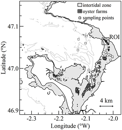
Figure 1. Bourgneuf Bay on the French Atlantic coast. Intertidal zone, oyster farms, and sampling stations are shown in gray, black, and white symbols, respectively. The location of the rectangle corresponds to the oyster farm's region of interest (ROI).

FIGURE 2

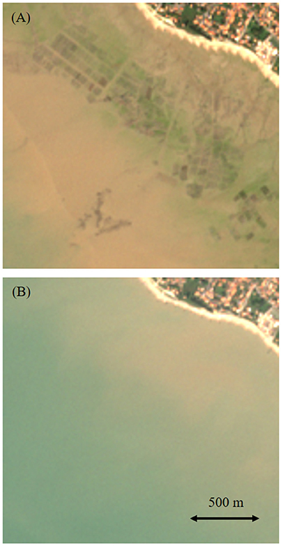
Figure 2. Rayleigh-corrected Sentinel2 Red Blue Green (RGB) image of the oyster farming site during low tide the 30 September 2015 (A), and during high tide the 15 March 2016 (B). The mudflat is emerged during low tide, and the oyster tables are visible from above. During high tide, oyster tables are not visible due to the extremely high turbidity.

In situ Data

Field data were acquired during two bio-optical cruises in Bourgneuf Bay from 08 to 12 April 2013 and from 12 to 13 April 2016 in the frame of the ANR GIGASSAT and FP7 HIGHROC projects, respectively. During both cruises, water sampling and radiometric measurements were performed following the same protocol. Sampling stations were located nearshore, mostly within the intertidal zone and in the vicinity of farming sites (Figure 1). Sampling took place at different times of the tidal cycle in order to acquire reflectance spectra over a wide range of SPM and chl a concentration. The same flat-bottomed barge was used during both cruises. This kind of vessel makes it possible to navigate throughout the shallow intertidal waters, even during low tide. Some stations were visited when the water depth was as low as 0.5 m. The bottom was never visible from above surface, even at the shallowest station due to the extremely high turbidity.

Radiometric Data

Above-water radiometric measurements were conducted following standard protocols (Mueller et al., 2000) to determine the spectral water-leaving radiance reflectance (also commonly referred as the marine reflectance), ρ_w(λ), defined as:

$\begin{array}{ll}{\rho }_w(\lambda )=\pi [L_u(\lambda )-{\rho }_{sky}{L}_{sky}(\lambda )]/E_d(\lambda )& (1)\end{array}$

where L_u (λ) is the upwelling radiance from the water and air-sea interface measured at a zenith angle of about 37°, L_sky(λ) is the sky radiance, ρ_sky is the air-water radiance reflection coefficient, E_d(λ) is the above-water downwelling irradiance, and λ is the wavelength. The barge was oriented away from the sun to avoid shadowing effects. Radiance sensors were pointed at a solar azimuth angle between 90 and 135°. The radiometric data were acquired simultaneously during about 5 min of stable sky conditions using three TriOS radiometers, two measuring the radiance signal and one measuring the downwelling irradiance.

A thorough quality control was made and only clear sky data were selected. Wave height was <0.5 m and wind speed was <5.0 m s⁻¹ during both cruises. The ρ_sky coefficient was taken as 0.02 following Austin (1974). The TriOS data were averaged over the time span of the measurement, smoothed over a 10 nm moving-window, cut within 400 and 900 nm (Figure 3A), and then spectrally downgraded at the resolution of the MSI onboard Sentinel2 using the spectral response function provided by the European Space Agency (Figure 3B).

FIGURE 3

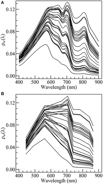
Figure 3. In situ marine reflectance ρ_w(λ) at TriOS (A), and Sentinel2 (B) spectral resolution.

Seawater Samples

Seawater samples were collected just below the surface concomitantly with radiometric measurements. Seawater samples were stored in 1 l bottles until they were filtered in the laboratory in the evening. The turbidity, T (in Formazin Nephelometric Unit, FNU), of each water sample was determined in triplicate using a 2100Q portable turbidimeter (Hach Company, Loveland, CO, USA) in order to optimize the volume of filtered seawater as in Neukermans et al. (2012). SPM, defined as the dry mass of particles per unit volume of seawater, was then determined using a standard gravimetric technique. Measured volumes of seawater (between 10 and 200 ml depending of the turbidity of the sample) were filtered through 25 mm diameter preweighed Whatman GF/F glass-fiber filters. At the end of filtration, sample filters were rinsed with deionized water to remove sea salt. The filters were frozen and shipped at the Laboratoire d'Océanographie de Villefranche (LOV). The dry mass of particles collected on the filter was then measured with a MT5 microbalance (Mettler-Toledo Intl. Inc.) with a resolution of 0.001 mg. A significant relationship between SPM and T was obtained (p < 0.01).

Depending on the turbidity, between 10 and 300 ml of seawater was also filtered through 25 mm GF/F filters for high performance liquid chromatography (HPLC) pigment analysis. The filters were frozen in liquid nitrogen and shipped for analysis at LOV, where HPLC analysis was performed according to Ras et al. (2008). The total chlorophyll a (chl a) concentration was computed as the sum of the “true” chlorophyll a, divinyl-chlorophyll a, and chlorophyllide a.

Bio-Optical Algorithms

Chlorophyll a Algorithm

Several algorithms are available for Sentinel2/MSI (Beck et al., 2016; Toming et al., 2016) to retrieve chl a concentration from ρ_w(λ) in coastal waters. For our study site, an intercomparison exercise based on in situ measurements demonstrates that the chlorophyll-retrieval algorithm of Gons et al. (2005) provided the most satisfactory results (see Supplementary Information for more details). This algorithm was originally developed for the Medium Resolution Imaging Spectrometer (MERIS) using the bands at 665, 705, and 775 nm (Gons, 1999; Gons et al., 2002, 2005). It was applied here to Sentinel2/MSI using bands B4 (665 nm), B5 (705 nm), and B7 (783 nm). Due to the shift from 775 to 783 nm, a recalibration has been performed to update the algorithm to Sentinel2/MSI. The chlorophyll-retrieval is done in three steps. First, the backscattering coefficient (b_b) is estimated from ρ_w at 783 nm:

$\begin{array}{ll}{b}_b(783)=1.56{\rho }_w(783)/\left[0.082-0.6{\rho }_w(783)\right]& (2\text{a})\end{array}$

Note that Equation (2a) is specific to Sentinel2/MSI, and replaces the original equation for MERIS:

$\begin{array}{ll}{b}_b(775)=1.61{\rho }_w(775)/\left[0.082-0.6{\rho }_w(775)\right]& (2\text{b})\end{array}$

Second, the phytoplankton absorption at 665 nm is retrieved from a NIR/red band ratio:

$\begin{array}{ll}{a}_{phy}(665)=(0.70+b_b){\rho }_w(705)/{\rho }_w(665)-0.40-b_b^p& (3)\end{array}$

where p is a unitless tuning parameter. Third, chl a concentration is computed by division with the chlorophyll-specific absorption coefficient at 665 nm, $a_{phy}^{*}$(665):

$\begin{array}{ll}\left[\text{chl }a\right]=a_{phy}(665)/a_{phy}^{*}(665)& (4)\end{array}$

It is assumed in Equation (3) that b_b(λ) is spectrally neutral between 665 and 783 nm, and that at 665 nm the absorption by chlorophyll a and by pure seawater is much higher than the absorption by mineral particles and CDOM.

The parameters $a_{phy}^{*}$(665) and p were initially estimated using a large dataset of field measurements from diverse inland, estuarine and coastal waters (Gons, 1999; Gons et al., 2002, 2005). For our study site in Bourgneuf Bay, $a_{phy}^{*}$(665) was recalibrated to 0.133 m² (mg chl a)⁻¹ (standard error is 0.002 m² (mg chl a)⁻¹) and p to 1.02. The recalibration was done using a fitting procedure based on a root mean square error minimization (Figure 4).

FIGURE 4

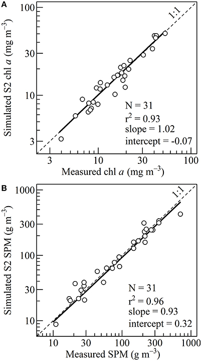
Figure 4. (A) Linear regression between the measured and simulated chlorophyll a concentration, obtained from in situ measurements. The thick line shows the fit between 4 and 52.5 mg m⁻³. The fit was used to calibrate the Gons et al. (2005) algorithm. (B) Linear regression between the measured and simulated suspended particulate matter concentration, obtained from in situ measurements. The thick line shows the fit between 10 and 700 g m⁻³. The fit was used to calibrate the Novoa et al. (2017) algorithm.

SPM Algorithm

The SPM concentration was computed using a multi-conditional algorithm previously developed for Bourgneuf Bay and the Loire estuary (Novoa et al., 2017). This algorithm has been validated for the Operational Land Imager (OLI) onboard Landsat8 (Novoa et al., 2017). A spectral recalibration has been performed here so that the algorithm could be applied to Sentinel2/MSI using bands B4 (665 nm) and B8A (865 nm). The algorithm is based on a switching method that automatically selects the most relevant SPM vs. ρ_w relationship to avoid saturation effects at high turbidity. The final SPM concentration is computed as a dynamic combination of SPM retrievals in the red and NIR bands:

$\begin{array}{ll}\left[\text{SPM}\right]=\alpha {\left[\text{SPM}\right]}_{\text{red}}+\beta {\left[\text{SPM}\right]}_{\text{NIR}}& (5)\end{array}$

where [SPM]_red, [SPM]_NIR, α, and β are defined as:

$\begin{array}{llll}{\left[\text{SPM}\right]}_{\text{red}}& =& 297{\rho }_w(665)/\left[1-{\rho }_w(665)/0.1238\right]& (6)\end{array}$

$\begin{array}{llll}{\left[\text{SPM}\right]}_{\text{NIR}}& =& 4302{\rho }_w(865)/\left[1-{\rho }_w(865)/0.2115\right]& (7)\end{array}$

$\begin{array}{llll}\alpha & =& \text{log}\left[0.090/{\rho }_w(665)\right]/\text{ log}(0.090/0.046)& (8)\end{array}$

$\begin{array}{ll}\beta =\text{log}\left[{\rho }_w(665)/0.046\right]/\text{ log}(0.090/0.046)& (9)\end{array}$

Due to the shift from 655 nm (Landsat8/OLI) to 665 nm (Sentinel2/MSI) the coefficients used in Equation 6 were recalibrated for Sentinel2/MSI using a fitting procedure based on a root mean square error minimization (Figure 4). The coefficients used in Equations (7–9) are the initial values computed by Novoa et al. (2017).

Satellite Data and Processing

Atmospheric Correction

Ortho-rectified, geo-located, and radiometrically calibrated top-of-atmosphere (TOA) reflectance Sentinel2 images were downloaded in the SAFE format from the US Geological Survey web portal (https://earthexplorer.usgs.gov). A single scene can contain multiple granules (sub-tiles), but the USGS web portal makes it possible to directly download Sentinel2 data at granule level, thus reducing downloading and processing time. Sentinel2 TOA data was processed using the ACOLITE software (http://odnature.naturalsciences.be/remsem/software-and-data/acolite) to derive the water-leaving radiance. This software proposes two options for the atmospheric correction (AC): (i) the NIR algorithm based on the assumption of spatial homogeneity of the red/NIR ratio for aerosol and marine reflectance (Ruddick et al., 2000; Vanhellemont and Ruddick, 2014) using Sentinel2 spectral bands at 665 and 865 nm, (ii) and the SWIR algorithm based on the assumption of zero water-leaving reflectance in the SWIR, using Sentinel2 spectral bands at 1,610 and 2,190 nm (Vanhellemont and Ruddick, 2015, 2016). ACOLITE establishes a per-tile aerosol type (or epsilon) as the ratio between the Rayleigh corrected reflectance in the two aerosol correction bands, for pixels where the marine reflectance can be assumed to be zero (i.e., where ρ_w(665 nm) <0.005, as defined by Vanhellemont and Ruddick, 2014). The epsilon is then used to extrapolate the observed aerosol reflectance to the NIR and visible bands. For the SWIR algorithm, ACOLITE also provides a choice for aerosol correction using a fixed epsilon over the region of interest (ROI), or a per pixel variable epsilon.

As the NIR AC option is not adapted to turbid waters (Vanhellemont and Ruddick, 2015), we used here the SWIR AC option with a fixed epsilon over the ROI, as recommended by several authors (Van der Zande et al., 2016; Novoa et al., 2017; Tristan Harmel, personal communication). The ROI was taken as Bourgneuf Bay and the Loire estuary (i.e., longitude from −2.35 to −1.95°E, and latitude from 46.85 to 47.35°N). The atmospheric correction is then performed in two steps: (i) a Rayleigh correction for scattering by air molecules using a look-up table generated using 6SV (Vermote et al., 2006), and (ii) an aerosol correction based on the assumption of black water reflectance in the SWIR bands due to the extremely high pure-water absorption, and an exponential spectrum for multiple scattering aerosol reflectance. Due to the low signal in the SWIR wavelengths, a spatial smoothing filtering for these bands was performed (Vanhellemont and Ruddick, 2016)

The final output of ACOLITE software is the ρ_w(λ) data in Network Common Data Form (NetCDF). SPM and chl a concentrations were then computed from ρ_w(λ) using the R project for statistical computing (R Development Core Team, 2008).

Selection, Clustering, and Sorting of Satellite Data

In intertidal waters, the spatio-temporal distribution of in-water suspended constituents is mainly driven by tidal dynamics. A total of 12 clear sky images was selected in order to observe the oyster farming site over a variety of seasonal, hydrological, and tidal conditions (Table 1). The time difference between satellite observation and low tide varied from <1 h to more than 5 h, thus providing a set of images acquired from low to high tide. The water height at the nearest reference harbor varied between 0.93 and 4.43 m, and the oyster farming site was observed over a variety of tidal configurations, from almost full emersion to complete submersion.

TABLE 1

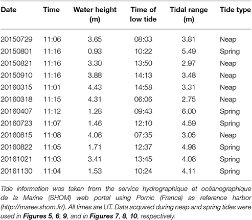
Table 1. Sentinel2 data used in the present study.

During the selected days of satellite acquisition the tidal range varied from 2.75 to 6 m, encompassing neap and spring tides (Table 1). The dataset was then divided in two subsets according to the tidal amplitude so that images were either clustered into neap tide (tidal amplitude <4 m) or into spring tide (tidal amplitude >4 m).

Irrespective of their acquisition date, Sentinel2 data were tidally sorted from ebb tide to flow tide according to the time difference between satellite observation and low tide, and to the water height at the time of acquisition. Sentinel2-derived SPM and chl a concentration maps were thus clustered in 2 composite tidal cycles, either representative of neap or spring tide. In order to investigate the influence of changes in SPM and chl a concentration on oysters, several physiological functions were directly retrieved from satellite data, as described below.

Simulating Oyster Physiology from Space

Oyster clearance rate was computed from SPM concentration as in Barillé et al. (1997) using a non-linear function response (see also Figure 3 in Gernez et al., 2014). Briefly, oyster clearance rate is constant and equal to 4.8 L h⁻¹ when SPM concentration is lower than 60 g m⁻³. Over this threshold the clearance rate is negatively impacted by the high turbidity. It follows a linear and decreasing trend between 60 and ~200 g m⁻³, and exponentially collapses over ~200 g m⁻³. This latter point corresponds to the saturation of the oyster gills (Barillé et al., 1997). The chlorophyll consumption rate, defined as the biomass of chl a consumed per hour, is then computed as the product of the chl a concentration by the clearance rate (Barillé et al., 1997):

$\begin{array}{ll}\text{CONS}={\left[\text{chl }a\right]}^{.}\text{CR}& (10)\end{array}$

where CR and CONS are, respectively the oyster clearance and chlorophyll consumption rates.

The clearance and chl consumption rates were simulated for each pixel of the Sentinel2 images using satellite-derived SPM and chl a data. In order to analyze the influence of the tide-driven chl a and SPM dynamic on oyster physiological response, composite tidal cycles of the clearance and chl consumption rates were also computed for the neap tide and spring tide clusters.

Results

In situ Reflectance Spectra

In situ hyperspectral marine reflectance spectra show some typical characteristics of coastal turbid waters (Figure 3A). From 400 to 580 nm ρ_w(λ) is relatively insensitive to changes in SPM and chl a concentration, preventing the use of a blue to green ratio algorithm to derive chl a concentration. From 600 to 900 nm the changes in the magnitude and spectral composition of the marine reflectance are mainly driven by variation in SPM concentration, notably as a result of particulate scattering.

In the red and NIR spectral region, the ρ_w spectra also display several features associated with the presence of pigment-bearing particles. An inflection in the reflectance slope is visible around 632 nm, attributable to the absorption by both chl a and chl c, a pigments association specific to diatoms (Méléder et al., 2005). The most striking feature is however the trough at 675 nm associated with chl a absorption, and the resulting reflectance shift between 675 and 700 nm, generally referred to as the NIR/red edge (Gons et al., 2002). Significant chl a concentration was confirmed by the analysis of HPLC data. It most likely originates from the tide-driven resuspension of benthic microalgae resuspended together with surface sediments.

Though a significant loss of information results from the downscaling of the TriOS hyperspectral reflectance to S2/MSI spectral resolution, a NIR/red edge between 665 and 705 nm is still noticeable on several S2-simulated ρ_w spectra (Figure 3B), making it possible to apply the Gons et al. (2005) algorithm in Bourgneuf Bay's intertidal waters.

In situ Calibration of the SPM and Chl a Algorithms

The SPM and chl a in situ data acquired concomitantly with the ρ_w(λ) were used to calibrate the bio-optical algorithms using a fitting procedure (Figure 4). In situ SPM concentration ranged from 10.92 to 700.83 g m⁻³, with a mean of 146.53 g m⁻³. Over this range, a significant relationship was obtained between simulated and measured SPM concentration (p-value < 10⁻⁵, correlation coefficient of 0.96, a slope of 0.93 and an intercept of 0.32). For the SPM retrieval, the root mean square error was 56.26 g m⁻³.

The range of chl a concentration was from 3.97 to 52.51 mg m⁻³, with a mean of 18.48 mg m⁻³. In the initial algorithm of Gons et al. (2005), the chlorophyll-retrieval parameters were originally set to p = 1.05 and $a_{phy}^{*}$(665) = 0.014 m² (mg Chl a)⁻¹ using observations performed in a variety of inland, estuarine and coastal waters over a range of chl a concentration from 1 to 181 mg m⁻³ (Gons, 1999; Gons et al., 2002). For the present study p was recalibrated to 1.02. A mean $a_{phy}^{*}$(665) of 0.013 m² (mg Chl a)⁻¹ was obtained, a value consistent with previously reported specific absorption coefficients for the Saint Laurent Estuary (Bricaud et al., 1995), and for the Baltic and North seas (Babin et al., 2003). The comparison between the marine reflectance- and HPLC-derived chl a concentration was satisfactory (Figure 4A). The obtained linear regression shows a significant correlation coefficient of 0.93 (p-value < 10⁻⁵), a slope of 1.02 and an intercept of −0.07. For the chl retrieval, the root mean square error was 3.05 mg m⁻³.

Chl a Concentration within the Oyster Farm

The high spatial resolution (20 m) and spectral characteristics of Sentinel2 made it possible to quantify the distribution of SPM and chl a concentration at the scale of an oyster farm (Figures 5–8). Three main features characterized SPM and chl a spatial distribution in the shellfish farming site. First, both SPM and chl a concentrations are generally high, often exceeding 200 g m⁻³ and 10 mg m⁻³, respectively. Second, their spatial structure depends on the bathymetry. SPM and chl a concentrations generally increase coastward, and the changes observed in their spatial distribution are more or less parallel to the isobaths (see for examples Figure 6C where the change in [chl a] from <5 to >10 mg m⁻³ occurred around the 1 m isobath, and Figure 7D where [SPM] displayed a clear gradient coastward). Third, the tidal cycle is a significant driver of SPM and chl a dynamics. Due to the tidal resuspension of benthic microalgae together with the other particles of the sedimentary surface, the chl a distribution was generally associated with SPM, a common feature of intertidal mudflats (Koh et al., 2006). Spatial fronts of highest chl a concentration generally move seaward during ebb tide (Figures 6A–C, 8A–C), and coastward during flow tide (Figures 6D–F, 8D–F).

FIGURE 5

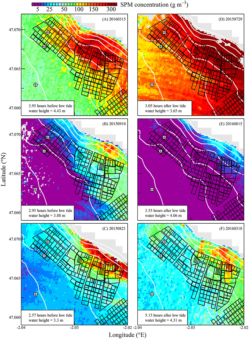
Figure 5. Suspended particulate matter concentration during neap tides. Sentinel2 data were sorted following a composite tidal cycle from ebb tide (A–C) to flow tide (D–F). Time difference between Sentinel2 acquisition and low tide is indicated, as well as the water height at the nearest reference harbor. The black polygons show the location of oyster tables. The white lines show the isobaths from 0 to 6 m above chart datum. The emerged part of the intertidal zone is in gray. Circled crosses around isobaths 0, 1, and 2 m show the points for which oyster clearance and consumption rates were computed (see Figures 9, 10).

FIGURE 6

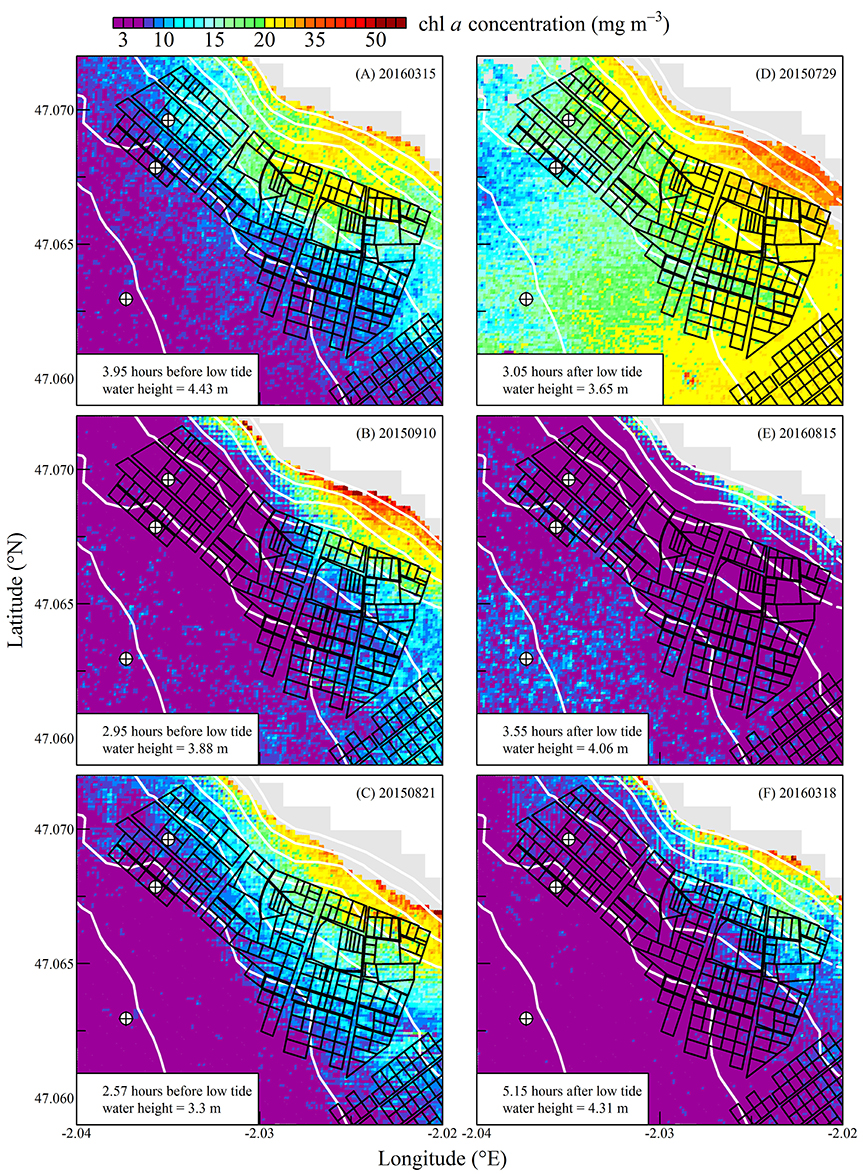
Figure 6. Same as for Figure 5 but for chlorophyll a concentration.

FIGURE 7

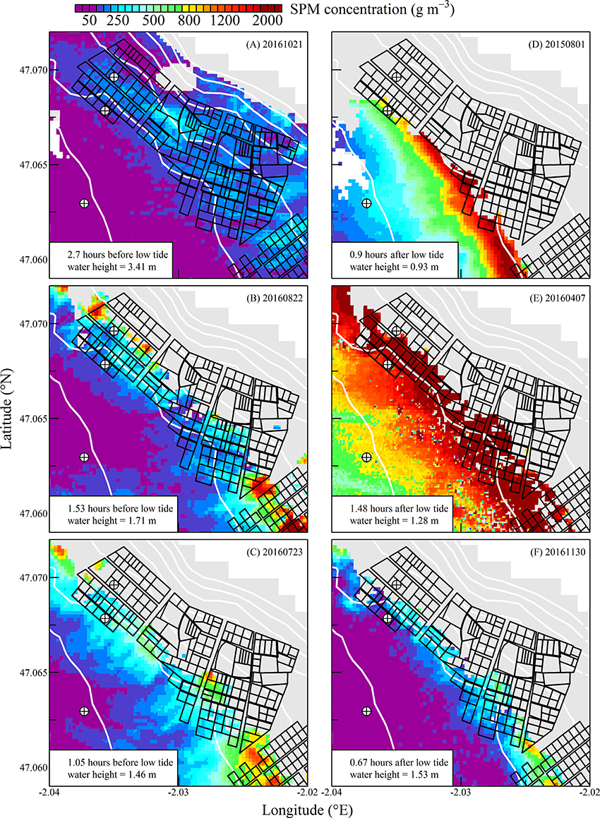
Figure 7. Same as for Figure 5 but during spring tides. Note the change in the color scale.

FIGURE 8

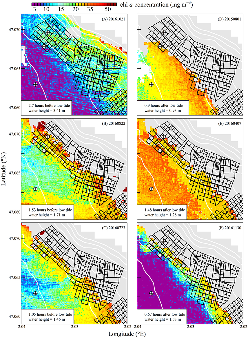
Figure 8. Same as for Figure 6 but during spring tides.

SPM and chl a concentrations exhibited similar spatial pattern during neap tide and spring tides, but the amplitude of the changes in their concentrations varied markedly between neaps and springs. For example, within the oyster farming zone SPM concentration varied from <10 to 300 g m⁻³ during neap tides and from 50 to >1,000 g m⁻³ during spring tides. Chl a concentration varied from <5 to 25 mg m⁻³ during neap tides and from 10 to 40 mg m⁻³ during spring tides.

The tide-driven variability was confirmed by the analysis of SPM and chl a concentration at the three selected fixed locations (black circled crosses in Figures 5–8). Both SPM and chl a concentration increased during ebb tide, reaching their maximum value during low tide and the start of the flow tide, and eventually decreasing during the end of the flow tide (Figures 9A,C, 10A,C). The temporal correlation between SPM and chl a concentration is attributable to the tide-driven resuspension of surface sediments, which contain both mineral particles and benthic microalgae. As expected, the amplitude of the tide-driven changes in SPM and chl a was higher during spring than during neap tides.

FIGURE 9

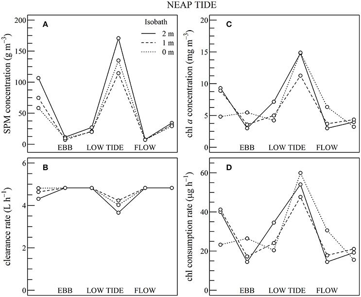
Figure 9. Using Sentinel2 data shown in Figures 5, 6, composite tidal cycle of suspended particulate matter (SPM) concentration (A), oyster clearance rate (B), chlorophyll a (chl a) concentration (C), and chl consumption rate (D) during neap tides at three bathymetric locations, as indicated.

FIGURE 10

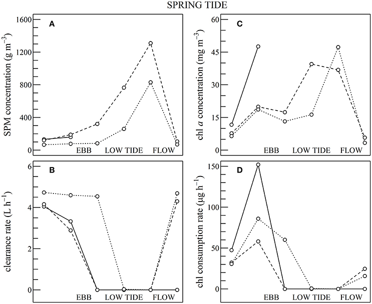
Figure 10. Same as for Figure 9 but using Sentinel2 data shown in Figures 7, 8, during spring tides.

The temporal changes in clearance and chl consumption rates were then analyzed in order to quantify the influence of the tide-driven SPM and chl a dynamic on the oyster physiological responses.

Influence of SPM and Chl a Variation on Oyster Physiology

During neap tides the simulated chl consumption rate mirrored the changes observed in chl a concentration (Figures 9C,D). This is attributable to the limited negative impact of SPM concentration on the clearance rate (Figures 9A,B). Generally SPM concentration remained below 100 g m⁻³ throughout the composite tidal cycle, except during flow tide where SPM concentration increased up to 175 g m⁻³ due to the erosion of surface sediments by tidal currents. The clearance rate mostly fluctuated between 4 and 5 L h⁻¹, and the decrease which occurred just after low tide was too small to counterbalance the increase in chl consumption.

During spring tides the simulated oyster physiological functions were more complexly affected by SPM and chl a tidal variability (Figure 10). First, a significant part the intertidal zone rapidly became emerged, and after mid-ebb the oysters could no longer filter seawater nor consume particles (see plain lines in Figure 10). In the waters just outside the intertidal zone, SPM concentration rapidly exceeded 200 g m⁻³ due to the strong tidal currents occurring from mid-ebb to the end of flow tide (dashed and dotted lines in Figure 10A). Such high SPM concentrations are known to saturate the oyster gills (Barillé et al., 1997), and it resulted in the dramatic collapse of the clearance rate from mid-ebb to the end of flow tide (Figure 10B). Meanwhile, the positive effects of the tide-driven increase in chl a concentration were rapidly counterbalanced by the collapse of the clearance rate, and the chl consumption rate dropped to zero from mid-ebb to the end of the flow (Figure 10D).

In summary, during neap tide, the tidal cycle in SPM concentration does not negatively impact oyster physiological response very much, and the low-tide increase in chl a concentration was directly translated into an increase in chl consumption for the farmed oysters. As most of the intertidal zone remains immerged during neap tides, the altitudinal location of the oyster farms has little influence on the tidal cycle of the clearance and chl consumption rate (Figure 9). During spring tides on the contrary, a significant fraction of the intertidal zone is emerged. In the waters adjacent to the intertidal zone and in the intertidal areas still under water, the high SPM concentration negatively impacts both clearance and chl consumption rate, whatever the chl a concentration, thus further limiting oyster physiological activity during a significant fraction of the tidal cycle (Figure 10).

Discussion

Chl a Algorithms in Turbid Coastal Waters

The Gons et al. (2005) algorithm, recalibrated to Sentinel2/MSI, was fitted to in situ measurement (Figure 4) before being applied to Bourgneuf Bay. The fit was satisfactory, as demonstrated by the consistency of the value of $a_{phy}^{*}$(665) with the literature (Bricaud et al., 1995; Gons et al., 2002; Babin et al., 2003). Other algorithms could have been used. Besides the Gons et al. (2005) method, various approaches were previously developed for turbid and/or eutrophic coastal and inland waters, including the 2-, and 3-band models (Dall'Olmo et al., 2005; Gitelson et al., 2008; Le et al., 2013), the fluorescence line height (FLH, Gower et al., 1999), the maximum chlorophyll index (MCI, Gower et al., 2005), and the 705 nm peak height (Toming et al., 2016). These algorithms are all based on a NIR/red edge either associated with chl a absorption at 675 nm or with sun-induced chl a fluorescence. An obvious limitation of these NIR/red algorithms is the lack of sensitivity in waters where the reflectance trough associated with chl a absorption around 675 nm is hardly pronounced (see for example the lowest ρ_w(λ) spectrum in Figure 3). In less eutrophic waters (i.e., chl a concentration smaller than ~4 mg m⁻³), the use of blue-green wavelengths would be more relevant to retrieve chl a concentration.

A recent study demonstrated that the 2- and 3-band models (Dall'Olmo et al., 2005) worked well with simulated Sentinel2/MSI-like imagery (Beck et al., 2016). In our algorithm inter-comparison (see Supplementary Information), the most performant method for our study site was the Gons et al. (2005) algorithm. Besides its good performance, another advantage of the Gons et al. (2005) algorithm is that the p and $a_{phy}^{*}$(665) parameters seem to be relatively stable over a variety of coastal waters, including the numerous inland, estuarine, and coastal sites initially sampled by Gons (1999), and the intertidal waters of Bourgneuf Bay. Additional field data are however needed to assess the geographical robustness of a common set of parameters, as well as its seasonal stability. While the range of chl a concentration retrieved from Sentinel2 data in our study site was consistent with previous field measurements (Barillé-Boyer et al., 1997), the accuracy of the chl a concentration maps is more difficult to quantitatively appraise due to the lack of validation data. More in situ and match-up data are needed to improve the method.

Advantages and Limitations of Sentinel2 for Aquaculture Applications

The retrieval of chl a concentration using a NIR/red algorithm is relevant in eutrophic waters, but at lower chl a concentration the accuracy would probably decrease. It is then generally advised to switch toward shorter wavelengths in the blue-green parts of the visible spectrum. As far as Sentinel2 is concerned, the lack of a spectral band at around 412 nm will certainly limit the performance of chl a inversion methods, as it has been long demonstrated that such a spectral band improves the deconvolution of chl a, PIM, and CDOM absorption (Carder et al., 1999). For sensors equipped with a spectral band at 412 nm such as MERIS, the ocean color 5 (OC5) algorithm (Gohin et al., 2002) has been recently recommended in recent intercomparison studies of the North West European (Tilstone et al., 2017) and Vietnamese (Loisel et al., 2017) coastal waters. As already indicated by Vanhellemont and Ruddick (2016), several other limitations specific to Sentinel2 can also arise, due to its relatively wide bands, low signal-to-noise ratio, and lack of vicarious calibration.

Despite these issues, Sentinel2 offers four main advantages for the remote-sensing of shellfish farming ecosystems. First, its high spatial resolution (20 m) made it possible to observe aquaculture sites located nearshore, in narrow bays and estuaries (Gernez et al., 2014), and to analyze within-farm spatial variability. Second, its relatively small revisit time (which is now 5 days since the launch of Sentinel-2B) increases the probability of acquiring cloud-free data over a given site. Sentinel2 acquisition frequency also limits subsampling and observation biases for the study of rapidly varying environments. There is no doubt that the Sentinel2 time-series will strengthen observation robustness and statistical descriptors of the very dynamic and changing coastal waters. Third, its SWIR spectral band facilitates atmospheric correction over turbid waters (Vanhellemont and Ruddick, 2015). Fourth, its spectral resolution in the red and NIR spectral regions made it possible to apply a variety of chlorophyll inversion algorithms (see previous section). Altogether, these characteristics represent a significant improvement for the remote sensing of turbid oyster farming ecosystems, and more generally for coastal zone observation.

Shellfish Ecology from Space?

The combination of EO and shellfish physiological models opens new perspectives for aquaculture management, shellfish farming ecosystems studies (Gernez et al., 2014), and more broadly for a better understanding of the coastal ocean response to global changes. For example, the poleward extent of the Pacific oyster (a well-known invasive species, Herbert et al., 2016) along the European coasts has been recently quantitatively analyzed using an original coupling of EO with mechanistic physiological oyster modeling (Thomas et al., 2016). In another recent study the EO time-series archive has been used with climatic, biological and energetics models to better understand predicted changes in growth, reproduction and mortality risk for commercially and ecologically important bivalves in the Mediterranean Sea (Montalto et al., 2016).

Concurrently with the increase of EO aquaculture applications, the development of improved satellite products should not be neglected. The detection of phytoplankton species causing harmful algal blooms (HABs) is a major concern for fisheries and shellfish farming management (Sourisseau et al., 2016), and recent algorithm developments have proved useful to provide early warnings (Davidson et al., 2009) or statistical estimation of HAB-related risks (Kurekin et al., 2014). Enhanced characterization of the composition of the particulate assemblage could also be used to improve satellite-derived aquaculture products. For example, as oysters have the ability to preferentially select organic rather than mineral particles before ingestion (Barillé et al., 1997; Dutertre et al., 2009), estimation of the organic fraction of the particulate assemblage (Woźniak et al., 2010) could be used to better constrain shellfish physiological models.

Conclusion

In summary, it has been demonstrated that Sentinel2/MSI has the potential to map chlorophyll a and SPM concentration in turbid, chlorophyll-rich, intertidal waters. Sentinel2 high spatial resolution (20 m) made it possible to analyze SPM and chl a distribution at the scale of an oyster farm, thus opening new opportunities for aquaculture applications. The influence of the tidal dynamic on SPM and chl a concentration was highlighted, and its influence on oyster physiological response was analyzed in the shellfish farm and adjacent nearshore waters. During neap tides oysters were little influenced by the high turbidity, whereas during spring tides their clearance and chl consumption rates were significantly impacted by the extremely high SPM concentration during a significant fraction of the tidal cycle. This study confirms the potential of EO for marine spatial planning (Ouellette and Getinet, 2016), and offers a generic framework where the combination of high resolution satellite remote sensing with bivalves ecophysiological model makes it possible to explore the response of cultivated suspension feeders to environmental conditions in many coastal areas, and to optimize site selection for shellfish farming.

Author Contributions

All authors contribute to work design, data acquisition, and data interpretation. PG processed the data and wrote the manuscript. All authors gave their approval to the manuscript final version.

Funding

This work has been supported by the “Programme National de Télédétection Spatiale” (PNTS, http://www.insu.cnrs.fr/pnts) in the frame of the TURBO project (grant n° PNTS-2015-07), by the French Research National Agency (ANR) in the frame of the GIGASSAT project (grant n° ANR-12-AGRO-0001, http://www.gigassat.org/), by the European Union's Research and Innovation FP7 program in the frame of the HIGHROC project (grant n° 606797, http://www.highroc.eu/), and by the Tools for Assessment and Planning of Aquaculture Sustainability (TAPAS) project, a Horizon 2020 Research and Innovation Action funded by the European Commission (Grant agreement No: 678396, http://tapas-h2020.eu/).

Conflict of Interest Statement

The authors declare that the research was conducted in the absence of any commercial or financial relationships that could be construed as a potential conflict of interest.

Acknowledgments

The European Space Agency is acknowledged for the production and distribution of Sentinel2 data. The US Geological Survey is thanked for maintaining the earth explorer web portal (https://earthexplorer.usgs.gov). Morgane Larnicol and Stéfani Novoa are thanked for their participation to field work. The authors thank Quinten Vanhellemont and Kevin Ruddick for making the ACOLITE software freely available. The organizers of the CLEO workshop and special issue are thanked for their efforts to federate the ocean color scientific community. Emmanuel Devred and Zhubin Zheng are thanked for their comments.

Supplementary Material

The Supplementary Material for this article can be found online at: https://www.frontiersin.org/article/10.3389/fmars.2017.00137/full#supplementary-material

References

Austin, R. W. (1974). “Inherent spectral radiance signatures of the ocean surface,” in Ocean Color Analysis, eds S. Q. Duntley, R. W. Austin, W. H. Wilson, C. F. Edgerton, and S. W. Moran (San Diego, CA: Scripps Inst. of Oceanogr), 195.

Babin, M., Stramski, D., Ferrari, G. M., Claustre, H., Bricaud, A., Obolensky, G., et al. (2003). Variations in the light absorption coefficients of phytoplankton, nonalgal particles, and dissolved organic matter in coastal waters around Europe. J. Geophys. Res. Oceans 108, 3211. doi: 10.1029/2001jc000882

CrossRef Full Text | Google Scholar

Barillé, L., Héral, M., and Barillé-Boyer, A.-L. (1997). Modélisation de l'écophysiologie de l'huître Crassostrea gigas dans un environnement estuarien. Aquat. Living Res. 10, 31–48. doi: 10.1051/alr:1997004

CrossRef Full Text | Google Scholar

Barillé-Boyer, A.-L., Haure, J., and Baud, J.-P. (1997). L'ostréiculture en baie de Bourgneuf, Relation Entre la Croissance des Huîtres Crassostrea Gigas et le Milieu Naturel: Synthèse de 1986 à 1995. IFREMER Rep. DRV/RA/RST/97-16. Available online at http://archimer.ifremer.fr/doc/00000/1633/.

Beck, R., Zhan, S., Liu, H., Tong, S., Yang, B., Xu, M., et al. (2016). Comparison of satellite reflectance algorithms for estimating chlorophyll-a in a temperate reservoir using coincident hyperspectral aircraft imagery and dense coincident surface observations. Remote Sens. Environ. 178, 15–30. doi: 10.1016/j.rse.2016.03.002

CrossRef Full Text | Google Scholar

Blondeau-Patissier, D., Gower, J. F., Dekker, A. G., Phinn, S. R., and Brando, V. E. (2014). A review of ocean color remote sensing methods and statistical techniques for the detection, mapping and analysis of phytoplankton blooms in coastal and open oceans. Prog. Oceanogr. 123, 123–144. doi: 10.1016/j.pocean.2013.12.008

CrossRef Full Text | Google Scholar

Bricaud, A., Babin, M., Morel, A., and Claustre, H. (1995). Variability in the chlorophyll-specific absorption coefficients of natural phytoplankton: analysis and parameterization. J. Geophys. Res. Oceans 100, 13321–13332.

Google Scholar

Brito, A. C., Benyoucef, I., Jesus, B., Brotas, V., Gernez, P., Mendes, C. R., et al. (2013). Seasonality of microphytobenthos revealed by remote-sensing in a South European estuary. Cont. Shelf Res. 66, 83–91. doi: 10.1016/j.csr.2013.07.004

CrossRef Full Text | Google Scholar

Carder, K. L., Chen, F. R., Lee, Z. P., Hawes, S. K., and Kamykowski, D. (1999). Semianalytic moderate-resolution imaging spectrometer algorithms for chlorophyll a and absorption with bio-optical domains based on nitrate-depletion temperatures. J. Geophys. Res. Oceans 104, 5403–5421.

Google Scholar

Choy, E. J., Richard, P., Kim, K. R., and Kang, C. K. (2009). Quantifying the trophic base for benthic secondary production in the Nakdong River estuary of Korea using stable C and N isotopes. J. Exp. Mar. Biol. Ecol. 382, 18–26. doi: 10.1016/J.JEMBE.2009.10.002

CrossRef Full Text | Google Scholar

Dall'Olmo, G., Gitelson, A. A., Rundquist, D. C., Leavitt, B., Barrow, T., and Holz, J. C. (2005). Assessing the potential of SeaWiFS and MODIS for estimating chlorophyll concentration in turbid productive waters using red and near-infrared bands. Remote Sens. Environ. 96, 176–187. doi: 10.1016/j.rse.2005.02.007

CrossRef Full Text | Google Scholar

Davidson, K., Miller, P., Wilding, T. A., Shutler, J., Bresnan, E., Kennington, K., et al. (2009). A large and prolonged bloom of Karenia mikimotoi in Scottish waters in 2006. Harmful Algae 8, 349–361. doi: 10.1016/j.hal.2008.07.007

CrossRef Full Text | Google Scholar

Dessinges, M., Le Bihan, V., Le Goff, F., and Petit, M. (2012). Ostréiculture en Pays de la Loire. Carnet de bord n°5, CRC Pays de la Loire.

Dutertre, M., Beninger, P. G., Barillé, L., Papin, M., Rosa, P., Barillé, A. L., et al. (2009). Temperature and seston quantity and quality effects on field reproduction of farmed oysters, Crassostrea gigas, in Bourgneuf Bay, France. Aquat. Living Res. 22, 319–329. doi: 10.1051/alr/2009042

CrossRef Full Text | Google Scholar

Gernez, P., Barillé, L., Lerouxel, A., Mazeran, C., Lucas, A., and Doxaran, D. (2014). Remote sensing of suspended particulate matter in turbid oyster-farming ecosystems. J. Geophys. Res. Oceans 119, 7277–7294. doi: 10.1002/2014JC010055

CrossRef Full Text | Google Scholar

Gitelson, A. A., Dall'Olmo, G., Moses, W., Rundquist, D. C., Barrow, T., Fisher, T. R., et al. (2008). A simple semi-analytical model for remote estimation of chlorophyll-a in turbid waters: Validation. Remote Sens. Environ. 112, 3582–3593. doi: 10.1016/j.rse.2008.04.015

CrossRef Full Text | Google Scholar

Gohin, F., Druon, J. N., and Lampert, L. (2002). A five channel chlorophyll concentration algorithm applied to SeaWiFS data processed by SeaDAS in coastal waters. Int. J. Remote Sens. 23, 1639–1661. doi: 10.1080/01431160110071879

CrossRef Full Text | Google Scholar

Gons, H. J. (1999). Optical teledetection of chlorophyll a in turbid inland waters. Environ. Sci. Tech. 33, 1127–1132.

Google Scholar

Gons, H. J., Rijkeboer, M., and Ruddick, K. G. (2002). A chlorophyll-retrieval algorithm for satellite imagery (Medium Resolution Imaging Spectrometer) of inland and coastal waters. J. Plankton Res. 24, 947–951. doi: 10.1093/plankt/24.9.947

CrossRef Full Text | Google Scholar

Gons, H. J., Rijkeboer, M., and Ruddick, K. G. (2005). Effect of a waveband shift on chlorophyll retrieval from MERIS imagery of inland and coastal waters. J. Plankton Res. 27, 125–127. doi: 10.1093/plankt/fbh151

CrossRef Full Text | Google Scholar

Gower, J. F. R., Doerffer, R., and Borstad, G. A. (1999). Interpretation of the 685 nm peak in water-leaving radiance spectra in terms of fluorescence, absorption and scattering, and its observation by MERIS. Int. J. Remote Sens. 20, 1771–1786.

Google Scholar

Gower, J. F. R., King, S., Borstad, G., and Brown, L. (2005). Detection of intense plankton blooms using the 709 nm band of the MERIS imaging spectrometer. Int. J. Remote Sens. 26, 2005–2012. doi: 10.1080/01431160500075857

CrossRef Full Text | Google Scholar

Herbert, R. J. H., Humphreys, J., Davies, C. J., Roberts, C., Fletcher, S., and Crowe, T. P. (2016). Ecological impacts of non-native Pacific oysters (Crassostrea gigas) and management measures for protected areas in Europe. Biodivers. Conserv. 25, 2835–2865. doi: 10.1007/s10531-016-1209-4

CrossRef Full Text | Google Scholar

Jesus, B., Brotas, V., Ribeiro, L., Mendes, C. R., Cartaxana, P., and Paterson, D. M. (2009). Adaptations of microphytobenthos assemblages to sediment type and tidal position. Cont. Shelf Res. 29, 1624–1634. doi: 10.1016/j.csr.2009.05.006

CrossRef Full Text | Google Scholar

Kang, C. K., Lee, Y. W., Choy, E. J., Shin, J. K., Seo, I. S., and Hong, J. S. (2006). Microphytobenthos seasonality determines growth and reproduction in intertidal bivalves. Mar. Ecol. Prog. Ser. 315, 113–127. doi: 10.3354/meps315113

CrossRef Full Text | Google Scholar

Kazemipour, F., Launeau, P., and Méléder, V. (2012). Microphytobenthos biomass mapping using the optical model of diatom biofilms: application to hyperspectral images of Bourgneuf Bay. Remote Sens. Environ. 127, 1–13. doi: 10.1016/j.rse.2012.08.016

CrossRef Full Text | Google Scholar

Koh, C. H., Khim, J. S., Araki, H., Yamanishi, H., Mogi, H., and Koga, K. (2006). Tidal resuspension of microphytobenthic chlorophyll a in a Nanaura mudflat, Saga, Ariake Sea, Japan: flood–ebb and spring–neap variations. Mar. Ecol. Prog. Ser. 312, 85–100. doi: 10.3354/meps312085

CrossRef Full Text | Google Scholar

Kurekin, A. A., Miller, P. I., and Van der Woerd, H. J. (2014). Satellite discrimination of Karenia mikimotoi and Phaeocystis harmful algal blooms in European coastal waters: Merged classification of ocean colour data. Harmful Algae 31, 163–176. doi: 10.1016/j.hal.2013.11.003

PubMed Abstract | CrossRef Full Text | Google Scholar

Le, C., Hu, C., Cannizzaro, J., English, D., Muller-Karger, F., and Lee, Z. (2013). Evaluation of chlorophyll-a remote sensing algorithms for an optically complex estuary. Remote Sens. Environ. 129, 75–89. doi: 10.1016/j.rse.2012.11.001

CrossRef Full Text | Google Scholar

Loisel, H., Vantrepotte, V., Ouillon, S., Ngoc, D. D., Herrmann, M., Tran, V., et al. (2017). Assessment and analysis of the chlorophyll-a concentration variability over the Vietnamese coastal waters from the MERIS ocean color sensor (2002–2012). Remote Sens. Environ. 190, 217–232. doi: 10.1016/j.rse.2016.12.016

CrossRef Full Text | Google Scholar

MacIntyre, H. L., Geider, R. J., and Miller, D. C. (1996). Microphytobenthos: the ecological role of the “secret garden” of unvegetated, shallow-water marine habitats. I. Distribution, abundance and primary production. Estuaries 19, 186–201.

Google Scholar

Méléder, V., Barillé, L., Rincé, Y., Morançais, M., Rosa, P., and Gaudin, P. (2005). Spatio-temporal changes in microphytobenthos structure analysed by pigment composition in a macrotidal flat (Bourgneuf Bay, France). Mar. Ecol. Prog. Ser. 297, 83–99. doi: 10.3354/meps297083

CrossRef Full Text | Google Scholar

Méléder, V., Launeau, P., Barillé, L., and Rincé, Y. (2003). Microphytobenthos assemblage mapping by spatial visible-infrared remote sensing in a shellfish ecosystem. C. R. Biol. 326, 377–389. doi: 10.1016/S1631-0691(03)00125-2

CrossRef Full Text

Montalto, V., Helmuth, B., Ruti, P. M., Dell'Aquila, A., Rinaldi, A., and Sarà, G. (2016). A mechanistic approach reveals non linear effects of climate warming on mussels throughout the Mediterranean sea. Climatic Change 139, 293–306. doi: 10.1007/s10584-016-1780-4

CrossRef Full Text | Google Scholar

Mueller, J. L., Davis, C., Arnone, R., Frouin, R., Carder, K., Lee, Z. P., et al. (2000). “Above-water radiance and remote-sensing reflectance measurements and analysis protocols,” in Ocean Optics Protocols for Satellite Ocean Color Sensor Validation, Revision 3, eds G. S. Fargion and J. L. Mueller (Greenbelt, MD: NASA Goddard Space Flight Center), 171–182.

Neukermans, G., Ruddick, K., Loisel, H., and Roose, P. (2012). Optimization and quality control of suspended particulate matter concentration measurement using turbidity measurements. Limnol. Oceanogr. Meth. 10, 1011–1023. doi: 10.4319/lom.2012.10.1011

CrossRef Full Text | Google Scholar

Novoa, S., Doxaran, D., Ody, A., Vanhellemont, Q., Lafon, V., Lubac, B., et al. (2017). Atmospheric corrections and multi-conditional algorithm for multi-sensor remote sensing of suspended particulate matter in low-to-high turbidity levels Coastal Waters. Remote Sens. 9:61. doi: 10.3390/rs9010061

CrossRef Full Text | Google Scholar

Ouellette, W., and Getinet, W. (2016). Remote sensing for marine spatial planning and integrated coastal areas management: achievements, challenges, opportunities and future prospects. Remote Sens. Appl. Soc. Environ. 4, 138–157. doi: 10.1016/j.rsase.2016.07.003

CrossRef Full Text | Google Scholar

Paterson, D. M., Wiltshire, K. H., Miles, A., Blackburn, J., Davidson, I., Yates, M. G., et al. (1998). Microbiological mediation of spectral reflectance from intertidal cohesive sediments. Limnol. Oceanogr. 43, 1207–1221.

Google Scholar

Ras, J., Uitz, J., and Claustre, H. (2008). Spatial variability of phytoplankton pigment distributions in the Subtropical South Pacific Ocean: comparison between in situ and modelled data. Biogeosciences 5, 353–369. doi: 10.5194/bg-5-353-2008

CrossRef Full Text | Google Scholar

R Development Core Team (2008). R: A Language and Environment for Statistical Computing. Vienna: R Foundation for Statistical Computing. Available online at: http://www.R-project.org

Ruddick, K. G., Ovidio, F., and Rijkeboer, M. (2000). Atmospheric correction of SeaWiFS imagery for turbid coastal and inland waters. Appl. Opt. 39, 897–912. doi: 10.1364/AO.39.000897

PubMed Abstract | CrossRef Full Text | Google Scholar

Sourisseau, M., Jegou, K., Lunven, M., Quere, J., Gohin, F., and Bryere, P. (2016). Distribution and dynamics of two species of Dinophyceae producing high biomass blooms over the French Atlantic Shelf. Harmful Algae 53, 53–63. doi: 10.1016/j.hal.2015.11.016

PubMed Abstract | CrossRef Full Text | Google Scholar

Thomas, Y., Pouvreau, S., Alunno-Bruscia, M., Barillé, L., Gohin, F., Bryère, P., et al. (2016). Global change and climate-driven invasion of the Pacific oyster (Crassostrea gigas) along European coasts: a bioenergetics modelling approach. J. Biogeogr. 43, 568–579. doi: 10.1111/jbi.12665

CrossRef Full Text | Google Scholar

Tilstone, G., Mallor-Hoya, S., Gohin, F., Couto, A. B., Sá, C., Goela, P., et al. (2017). Which ocean colour algorithm for MERIS in North West European waters? Remote Sens. Environ. 189, 132–151. doi: 10.1016/j.rse.2016.11.012

CrossRef Full Text | Google Scholar

Toming, K., Kutser, T., Laas, A., Sepp, M., Paavel, B., and Nõges, T. (2016). First experiences in mapping lake water quality parameters with Sentinel-2 MSI imagery. Remote Sens. 8:640. doi: 10.3390/rs8080640

CrossRef Full Text | Google Scholar

Ubertini, M., Lefebvre, S., Gangnery, A., Grangeré, K., Le Gendre, R., and Orvain, F. (2012). Spatial variability of benthic-pelagic coupling in an estuary ecosystem: consequences for microphytobenthos resuspension phenomenon. PLoS ONE 7:e44155. doi: 10.1371/journal.pone.0044155

PubMed Abstract | CrossRef Full Text | Google Scholar

Underwood, G. J. C., and Kromkamp, J. C. (1999). Primary production by phytoplankton and microphytobenthos in Estuaries. Adv. Ecol. Res. 29, 93–153. doi: 10.1016/S0065-2504(08)60192-0

CrossRef Full Text | Google Scholar

van der Wal, D., Wielemaker-van den Dool, A., and Herman, P. M. (2010). Spatial synchrony in intertidal benthic algal biomass in temperate coastal and estuarine ecosystems. Ecosystems 13, 338–351. doi: 10.1007/s10021-010-9322-9

CrossRef Full Text | Google Scholar

Van der Zande, D., Vanhellemont, Q., and Ruddick, K. (2016). “Validation of Landsat-8/OLI for ocean colour applications with AERONET-OC sites in Belgian coastal waters,” in Ocean Optics Conference (Victoria, BC), 23–28.

Vanhellemont, Q., and Ruddick, K. (2014). Turbid wakes associated with offshore wind turbines observed with Landsat 8. Remote Sens. Environ. 145:105–115. doi: 10.1016/j.rse.2014.01.009

CrossRef Full Text | Google Scholar

Vanhellemont, Q., and Ruddick, K. (2015). Advantages of high quality SWIR bands for ocean colour processing: Examples from Landsat-8. Remote Sens. Environ. 161, 89–106. doi: 10.1016/j.rse.2015.02.007

CrossRef Full Text | Google Scholar

Vanhellemont, Q., and Ruddick, K. (2016). “ACOLITE For Sentinel-2: Aquatic Applications of MSI imagery,” in ESA Special Publication Presented at the ESA Living Planet Symposium held in Prague (Czechia), 9–13.

Google Scholar

Vermote, E., Tanré, D., Deuzé, J., Herman, M., Morcrette, J., and Kotchenova, S. (2006). Second Simulation of a Satellite Signal in the Solar Spectrum-Vector (6SV). 6S User Guide Version 3. Greenbelt, MD: NASA Goddard Space Flight Center.

Google Scholar

Woźniak, S. B., Stramski, D., Stramska, M., Reynolds, R. A., Wright, V. M., Miksic, E. Y., et al. (2010). Optical variability of seawater in relation to particle concentration, composition, and size distribution in the nearshore marine environment at Imperial Beach, California. J. Geophys. Res. Oceans 115:C08027. doi: 10.1029/2009jc005554

CrossRef Full Text | Google Scholar