Identifying the Relevant Local Population for Environmental Impact Assessments of Mobile Marine Fauna

Introduction

Applied wildlife research can improve the scientific basis for environmental impact assessment (EIA) by developing methodologies to evaluate impacts of human activities on wildlife (Morrison et al., 2006; Steidl and Powell, 2006; Bejder et al., 2009, 2012; Torres et al., 2016). However, for such evaluations to be effective, they must also be directed at an appropriate scale of biological organization for the species to be impacted by a proposed development or activity. Here, we describe a methodology to identify the relevant local population for EIA which is suitable for species that are continuously distributed and highly mobile.

While the procedural and formal requirements for EIA are often closely prescribed by statutes, regulations, and associated policy and guidance documents, there are often few specific requirements as to the scientific information necessary for EIA. While many jurisdictions have now developed policies or protocols for biodiversity surveys to allow for the identification of fauna and flora species that may be affected by a proposed development or activity, prescriptive guidelines for the conduct of field studies of human impacts on wildlife, as set by the administrative bodies having statutory responsibility for EIA, remain uncommon. As such, it is vital for wildlife researchers to identify best-practice methodologies for field-based impact assessment research, so as to encourage their use in studies undertaken to support EIAs.

Broadly speaking, the aim of EIA is to conduct a detailed assessment of the potential impacts of a proposed development or activity on a particular environment (including the biota occurring there) on which decision-makers can then rely in determining whether the proposed development or activity should be approved and, if so, with what conditions (Glasson et al., 2012). Ideally, the EIA process for a proposed development or activity should consider the range of possible impacts on wildlife in a manner that is species-, site-, and (if applicable) season-specific (Fox et al., 2006). If the assessment methods employed are inappropriate or are inadequately implemented, the EIA outcomes (typically an environmental impact statement or report) may be incomplete and inaccurate. An obvious example is an EIA based on sparse and opportunistic sighting data for a species (Bejder et al., 2012).

To adequately characterize the impact of a proposed development or activity on a particular species, it is necessary to identify the relevant local population which may be impacted (Brittingham et al., 2014; Bastos et al., 2016; Brown et al., 2016). In highly fragmented landscapes, the relevant local population may be straightforward to delineate because of the geographical separation between the area affected by the development and the nearest other sites where the species may be found. For example, the presence of physical barriers (natural or anthropogenic) or long distances between patches may limit dispersal and thus enable isolation of local populations (e.g., natural and anthropogenic barriers for cougars, Sweanor et al., 2000; land-clearing for wombats, Walker et al., 2008; geographical distance for sharks, Sandoval-Castillo and Beheregaray, 2015). In contrast, identifying the relevant local population may be more challenging if a species is highly mobile (and therefore able to disperse between even geographically distant sites) or displays migratory behavior (e.g., between breeding sites and feeding areas), or if it is continuously distributed across the land or seascape (DeYoung, 2007).

What constitutes a “local population” is an important though often under-considered aspect of impact assessment research. Some concept of a local population is often implicit in considerations of spatial scale and population structure for EIA. In one sense, the local population may simply comprise the total number of individuals that may be affected by the proposed development or activity. In the simplest scenario, an EIA could proceed on the basis of an estimate of the number of individuals present in the “patch” that the development or activity will affect (Total Individuals Affected). However, it will often be desirable (or necessary) to identify the relevant biological population that may be impacted, in the sense of a group of animals (or “sub-population”) that displays some meaningful degree of genetic, demographic, or spatial discreteness (Population Unit Affected). An effective EIA may therefore require information about population structure, so that decision-makers can evaluate the biological significance of potential impacts—e.g., will the development affect the viability of a distinct population (or population unit) or is the species continuously distributed across the impact area and its surrounds such that little or no population structure is present? A metapopulation framework is often applied to examine interactions between spatially distinct local populations (Levins, 1969; Hill et al., 1997; Moilanen and Nieminen, 2002).

Weak population structure is often expected for marine wildlife because of the lack of barriers to movement and the broad distributions of many marine species (Waples, 1998). Nonetheless, geographic features do exist in the marine environment that may act as natural boundaries and thus contribute to population structuring, such as between estuarine, coastal, and offshore habitats. Bottlenose dolphins (Tursiops spp.), for example, are known to exhibit population (and even species) structure across a gradient from protected inshore environments to deeper, more exposed offshore habitats. For example, estuarine bottlenose dolphins generally exhibit greater site fidelity and year-round residency, have stronger and more enduring associations with conspecifics than do bottlenose dolphins in coastal habitats, and may form distinct “communities” within particular estuaries or embayments (Quintana-Rizzo and Wells, 2001). A “community” has been defined as a set of individuals that is behaviorally discrete from neighboring communities and within which most individuals associate with other members of the community (Wells et al., 1987). We suggest that a dolphin community might constitute a relevant local population for the purposes of EIA, both in terms of comprising the total number of animals that might be affected by a proposed development (Total Individuals Affected) and in terms of representing a population unit of some biological significance (Population Unit Affected). However, the diversity and flexibility of mammalian social behavior can make it difficult to identify communities for dolphins and other social mammal species (both terrestrial and marine) (Cantor and Whitehead, 2013).

As nearshore environments such as embayments and estuaries are a focus point for coastal development, EIAs will often need to consider how proposed developments and activities will affect local dolphin populations. These environments contain shallow and protected habitats that allow bottlenose dolphins to reside year-round (Wells, 1986; Brusa et al., 2016). Prey availability in these environments is also more continuous and dependable (Elliott and Whitfield, 2011; McCluskey et al., 2016) than in open and coastal regions, where prey is distributed patchily and prey availability is dictated largely by oceanic physical processes (Silva et al., 2008). The key ecological and demographic characteristics of dolphin communities in estuaries and embayments differ from those in coastal areas—e.g., inshore communities tend to be small and to exhibit weak to moderate levels of dispersal and immigration (Titcomb et al., 2015). These characteristics influence their vulnerability or resilience to human impacts (Bejder et al., 2009; Pirotta et al., 2013).

Impact assessment research has been undertaken for a range of developments and activities that may impact on dolphins, including activities such as dredging and pile driving that may exert short-term impacts on dolphin populations (Dungan et al., 2012; Pirotta et al., 2013; Culloch et al., 2016) and those which are more enduring, such as the construction of permanent infrastructure (Jefferson et al., 2009; Cagnazzi et al., 2013). The coastal and estuarine waters of Perth (Western Australia) have experienced significant development for industrial and other commercial uses. Notably, the Swan Canning Riverpark (SCR) estuary bisects the city, threading through heavily developed residential and agricultural areas (Holyoake et al., 2010), and Cockburn Sound (CS), a sheltered embayment, contains Perth's main industrial area. Some developments in the region have involved short-term activities (e.g., pile driving activities conducted in the Inner Harbor of the Port of Fremantle, Salgado Kent et al., 2012; Paiva et al., 2015), while others are continuing impacts (e.g., year-round dredging for a shell-sand mining operation, Environmental Protection Authority, 2001). In addition, new developments may be undertaken in the near future (e.g., a proposed outer harbor development on Kwinana Shelf, (Western Australian Planning Commission, 2004); a desalination plant proposed for the northern metropolitan coast, Mercer, 2013). In many respects, these developments are exemplars of the types of developments which may impact on dolphins and other wildlife in coastal and estuarine environments.

In this paper, we: (a) describe a methodology to identify local populations of wildlife and then (b) examine its further application in evaluating possible impacts of proposed developments and activities. Firstly, we integrated social, ecological, and genetic data collected during longitudinal field study to identify relevant local populations of Indo-Pacific bottlenose dolphins (T. aduncus) within estuarine and coastal waters of Perth. We employed sampling methodologies that are robust and consistent with best-practice for long-term monitoring, abundance estimation and behavioral study of coastal dolphins [e.g., systematic line-transect survey, photo-identification over a 4-year period (2011–2015)] to: (1) assess social networks of bottlenose dolphins through estimates of the Half-Weight Index (HWI) and network analysis; (2) compare the role of sex composition and temporal stability of association in driving social organization within communities based on Lagged Association Rates (LAR) and preferred associations; (3) examine the spatial segregation of the social communities by assessing home-range overlaps in conjunction with bathymetry and habitat differences, to assess the residency patterns; and (4) evaluate the genetic relatedness within and between communities by estimating the relatedness between individuals within and between communities. Secondly, we considered the fine-scale population structure of bottlenose dolphins in the context of past, current, and proposed developments for the region to demonstrate how such information about local populations can also assist in evaluating the possible impacts of proposed developments and activities.

Materials and Methods

Study Area

The study area was located in the metropolitan waters of Perth (Western Australia), one of the fastest growing capital cities in Australia (Australian Bureau of Statistics, 2015). The study area encompassed 275 km² and extended from Rockingham to Scarborough along the coast and then inland to include part of the Swan Canning Riverpark (SCR), an estuarine reserve (Figure 1). Following a mark-recapture robust design (Chabanne et al., 2017), the study area was subdivided into four geographic regions with three that were defined by the topography and bathymetry of the coastal waters (from South to North, Figure 1): (1) Cockburn Sound (CS)—a semi-enclosed embayment with varying depth (<2 to >20 m) and with seagrass, sand, silt, or limestone substrates; (2) Owen Anchorage (OA)—an embayment with less than 10 m depth, except in the channel (max depth: 14.7 m), and with a substrate mainly consisting of shell-sand and seagrass; (3) Gage Roads (GR)—an open coastline typified by deep waters (>10 m), with sandy beaches, rocky reefs, and seagrass patches. The lower section of GR, also deeper (>20 m), is an anchoring area for ships before entering the Port of Fremantle. The SCR is a micro-tidal estuary which encompasses an area of about 55 km² and includes two river systems (Swan and Canning rivers) that join near the City of Perth before reaching the Indian Ocean through the Inner Harbor of the Port of Fremantle. While the estuary is mainly shallow (<10 m), the Inner Harbour section is maintained at 14 m through regular dredging activities (Figure 1B). With a Mediterranean climate, the estuary experiences marked temperature and salinity variations through the year, particularly when freshwater flow is weak.

FIGURE 1

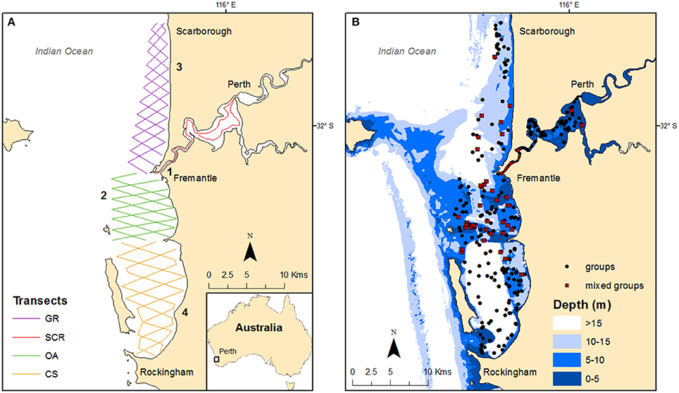
Figure 1. Maps of the study area showing: (A) the transect routes per geographic regions (GR, Gage Roads; SCR, Swan Canning Riverpark; OA, Owen Anchorage; CS, Cockburn Sound) with locations of past, current, and proposed developments (1- pile driving; 2- dredging; 3- desalination; 4- outer harbor); and (B) the bathymetry (in meters) with the locations of the groups sighted during the systematic surveys conducted from 2011 to 2015, including mixed groups (i.e., mix of individuals from different communities).

Data Collection

Boat-based surveys were conducted between June 2011 and May 2015 and within each season in the Australasian calendar (winter: June to August; spring: September to November; summer: December to February; autumn: March to May). Using boat-based photo-identification sampling, we documented individual bottlenose dolphins based on nicks and marks on the dorsal fin (Würsig and Jefferson, 1990). Three zig-zag transect routes (offset by 2 km) were designed using Distance 6.0 (Thomas et al., 2009) for each coastal geographic region in order to optimize the coverage (Figure 1A). Each route extended to ~7 km offshore in CS and OA and from 5 to 3 km offshore in GR. In the SCR, we followed the same transect route used during the 2001–03 study (Chabanne et al., 2012) which extended from the mouth of the estuary (Inner Harbour) through the lower reaches and the main basin where the Swan and Canning rivers join. Full details on the robust design sampling structure design and survey methodology (i.e., predefined transect routes, Figure 1A) are provided in Chabanne et al. (2017).

A cycle was defined as a successful completion of a survey within each geographic region of the study area. Our goal was to complete a cycle in a minimum period, although a minimum of 2 days was required because of daylight. During a survey, a sighting was defined as a group of dolphins observed within c. 250 m on either side of the boat along the transect route (Wells et al., 1987, 1999; Quintana-Rizzo and Wells, 2001). A group consisted of one to several dolphins. Dolphins were considered to be in a group if they were within 10 m of any individual within the group (a 10 m “chain” rule) and engaged in the same behavior (Smolker et al., 1992). For each sighting, we recorded the location (southing/easting using a hand-held GPS unit), behavior, group size, and age-sex composition. Age classes (adult, juvenile, and calf) were based on the body size or the presence of a dependent calf. Individuals were sexed through: (i) molecular analyses of tissue samples (Gilson et al., 1998; Brown et al., 2014) collected via remote biopsy sampling (Krützen et al., 2002); (ii) field observation of the genital regions; or (iii) the presence of a dependent calf (for females). We performed photo-identification using a Nikon D300 with Nikkor lens 70–300 mm or a D7000 with Nikkor lens 80–400 mm. Full details for photo-identification and grading processes are provided in Chabanne et al. (2017).

Association Patterns

To analyze patterns of association, we used only high-quality photographic identifications, from groups for which all individuals were identified. We did not consider the distinctiveness of the individuals to avoid small sample sizes. The survey frequency also allowed for use of temporary marks, if required. Individuals present in the same group were assumed to be associated (“gambit of the group”, Whitehead, 2008a). Calves were excluded from the analysis because they lack identifying marks, are dependent on their mothers and have high natural mortality (Mann et al., 2000). The sampling period was set to 1 day to minimize sampling time incoherency between successful surveys of the entire study area (i.e., a cycle). Individuals seen multiple times within the same cycle were restricted to the first sighting only. The strength of associations among dyads (i.e., pairs of individuals, n = 8,256) was calculated using the half-weight index (HWI, Cairns and Schwager, 1987). Values of HWI range from 0 (never associated) to 1 (always associated). The HWI is frequently used in social structure of cetaceans as it reduces bias due to incomplete identification within encounters (Cairns and Schwager, 1987). Only adults and juveniles sighted more than five times over the entire study period were retained for this analysis. The minimum number of sightings was decided by comparing the social differentiation (S, measure of variability of the associations) and Pearson's correlation coefficient (r, measure of the quality of the representation of the association pattern, Whitehead, 2008b) for different sets of data based on a minimum number of sightings per individual, until appropriate values were reached. Specifically, an S < 0.3 indicates that the society is homogeneous, 0.5 < S < 2 indicates that the society shows some strong associations between individuals, and S > 2 indicates that the society generally has weak associations between individuals (Whitehead, 2008b). Additionally, an r value near 1 indicates that the representation is excellent, while r ~ 0.8 suggests a good representation and r ~ 0.4 indicates a moderate representation (Whitehead, 2008b). All association patterns were analyzed using the software SOCPROG 2.6 (Whitehead, 2009).

A Monte Carlo permutation test was conducted to examine whether associations within the study area population were different from random (Bejder et al., 1998; Whitehead et al., 2005; Whitehead, 2008a). As such, a higher coefficient of variation (CV) of real association indices compared to that of randomly permuted data indicated the presence of preferred long-term companions in the studied population (Whitehead, 1999). We ran 1,000 permutations with 1,000 flips per permutation for the complete dataset and significant variations from random were tested using a two-tailed test (P-value = 0.05). The number of permutations was determined to be sufficient when the p-value stabilized (Bejder et al., 1998). The preferred associations are those for which an association index value is at least twice higher than the mean (Whitehead, 2008b). A Mantel test, using 1,000 permutations, was carried out to examine whether differences in associations occurred between sex classes (two-tailed 0.05 P-value, Schnell et al., 1985).

Community Structure and Dynamic

To investigate the social structure based on the HWI, we calculated the eigenvector modularity network algorithms to identify cut-off limits to identify possible communities (Newman, 2004, 2006). A modularity M > 0.3 indicated that the community division is meaningful (Newman, 2004; Whitehead, 2009). We used the software NetDraw 2.139 (Borgatti, 2002) to visualize the network structure. For comparison, we carried out an average linkage hierarchical cluster analysis that calculated a cophenetic correlation coefficient (CCC). A CCC of > 0.8 indicates a good match between the degree of association between individuals and the association matrix (Bridge, 1993).

We examined the association levels, some network measures, sex segregation and the temporal stability of associations to highlight potential differences in association patterns between the different communities identified. First, mean and maximum levels of associations were compared. Second, we measured the network strength, clustering coefficient and affinity within communities. The strength is the sum of the association indices of each individual, also defined as a measure of gregariousness (Barrat et al., 2004); the clustering coefficient indicates how well an individual's associates are themselves associated, and the affinity is a measure of the strength of an individual's associates (Whitehead, 2016). All the network measures were calculated in SOCPROG 2.6 (Whitehead, 2009). Thirdly, a Mantel test (as described above) was then carried out to examine whether differences in associations occur between sex classes within each community. Additionally, tests for preferred or avoided associations were run for each community and per sex classes as described above. And finally, we measured the persistence of associations within each community by calculating the lagged association rates (LAR, Whitehead, 1995). The LAR estimates the probability that two individuals sighted together at a given time will still be associated at some time lag later. LARs from each community were compared to the null LAR of the complete dataset (i.e., association value the animals would have if associating randomly, Whitehead, 1995). We then tested exponential decay models characterizing the patterns of dyadic association over time. The quasi-Akaike information criterion (QAIC) was used for model selection (Whitehead, 2007). We used the jackknife method to obtain estimates of precision of the LAR (Efron and Stein, 1981). LARs were also estimated and modeled as above for each sex class within each community.

Spatial Distribution of Communities

We calculated the estimates of kernel density (KDE) in ArcGIS 10.3 and estimated the probability of contours of 50% (i.e., the core of a community) and 95% (i.e., community's home range defined by the outermost boundaries) by pooling sightings of individuals assigned to the same community. Individuals that were equally observed in two or more geographic regions were excluded from this analysis. We used the kernel interpolation with barriers tool to take into account land barriers to movements (the output grid cell size was set to 200 × 200 m and the bandwidth was fixed to 6,000 for each individual, Sprogis et al., 2015). All other steps followed the protocols by MacLeod (2014) and were calculated in the Universal Transverse Mercator (UTM) Zone 50 South projection using the coordinate system World Geodetic System (WGS) 1984 datum. Overlaps in home ranges between each community were computed using the Intersect tool in ArcGIS. In order to characterize some factors associated with community structure, we also calculated an asymmetric matrix of pairwise individual home range (95% kernel density) overlaps following the same protocol as above and conducted a Mantel test (1,000 permutations) to check the correlation between home range overlaps and HWIs for each individual pairs between and within communities.

Residence Time

Using the software SOCPROG 2.6 (Whitehead, 2009), we assessed the demographic processes within each community by estimating the lagged identification rates (LIR) for each individual within their respective assigned community (Whitehead, 2001). This analysis estimated the probability that an individual would be resighted in the study area after a certain time lag (td) in comparison to a randomly chosen individual. We then fitted different models of no movement (i.e., closed population), emigration and mortality, emigration and reimmigration, and emigration, reimmigration and mortality to the observed LIR (Whitehead, 2001). We used the QAICc to select the most parsimonious model (Burnham and Anderson, 2002). The LIR confidence intervals (CI) were obtained using bootstrap replicates (Whitehead, 2008b).

Genetic Relatedness

Skin samples were collected via remote biopsy sampling (Krützen et al., 2002) over the 4-year period (2011–2015) mentioned earlier. However, additional samples collected between 2007 and 2010 were also included for genetic testing. All biopsy samples were stored in DMSO buffer for cryopreservation. Genomic DNA was extracted from all skin samples using the Gentra Puregene Tissue Kit (Qiagen) and following the manufacturer's protocol. Samples were genotyped at 13 different microsatellite loci: DIrFCB4, DIrFCB5 (Buchanan et al., 1996), LobsDi_7.1, LobsDi_9, LobsDi_19, LobsDi_21, LobsDi_24, LobsDi_39 (Cassens et al., 2005), SCA9, SCA22, SCA27 (Chen and Yang, 2008), TexVet5, TexVet7 (Rooney et al., 1999). We followed the PCR conditions as described in Frère C. H. H. et al. (2010). The single stranded PCR products were run on an ABI 3730 DNA Sequencer (Applied Biosystems). Genotypes were scored using Geneious v9.1.5 (http://www.geneious.com; Kearse et al., 2012) with microsatellite plugin 1.4 (Biomatters Ltd). Each microsatellite locus was checked for null alleles and scoring errors using the software Micro-Checker v2.2.3 with a confidence level of 95% (Van Oosterhout et al., 2004). Departures from Hardy-Weinberg equilibrium (HWE) and linkage equilibrium were tested using the Markov chain probability test and 10,000 iterations in Genepop v4.4.3 (Rousset, 2008). Significance values for multiple comparisons were adjusted by sequential Bonferroni corrections (Rice, 1989). We calculated individual pairwise relatedness within and between social communities using Queller and Goodnight (1989) Index (QG) in Coancestry v1.0.1.2 (Wang, 2011). Average relatedness coefficients within communities were tested using a t-test. We also conducted an ANOVA test to identify the correlation between pairwise relatedness and HWI within each community.

Ethics Statement

This study was carried out with approval from the Murdoch University Animal Ethics Committee (W2342/10, and R2649/14) and under licenses from the Western Australia Department of Parks and Wildlife (DPaW) (SF008067, SF008682, SF009286, and SF009874). Biopsy sampling for molecular analyses were carried out as a part of broader study, with data collected in accordance to the Murdoch University Animal Ethics Committee approval (W2076/07; W2307/10; W2342/10, and R2649/14), and collected under DPaW licenses (SF005997; SF006538; SF007046; SF007596; SF008480; SF009119: SF009734; SF010223).

Results

Effort and Group Size

A total of 322 group sightings were successfully (i.e., all individuals identified from good quality photos) obtained during the 4-year (2011–2015) study period. In total, 315 individual dolphins (excluding calves) were identified.

Average group size was 5 ± 0.27 (SE) individuals (range: 1–31 individuals) (Table 1). Although group size was similar across the three coastal geographic regions, it was smaller in SCR, with an average of four individuals and a maximum group size of 14 individuals).

TABLE 1

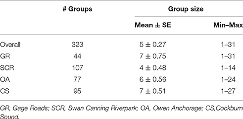
Table 1. Number of groups and group size (mean ± SE, minimum and maximum) by geographic region.

Community Structure and Dynamic

After restricting the dataset to those individuals with at least five sightings, 129 individuals were identified (n = 57 females, 44 males, and 28 unsexed). Both community division using the eigenvector method of Newman (2006) and modularity from gregariousness and hierarchical clustering using average linkage methods indicated a meaningful community division with maximum modularity of 0.514 and 0.526 for an HWI of 0.022 and a cophenetic correlation coefficient (CCC) of 0.843, indicating a good match between the degree of association between individuals and the association matrix. Both methods assigned individuals to four communities, although one community was split into two sub-communities (D and D'). From here on, we refer to these communities as ComA, ComB, ComC, and ComD. Three individuals (designated as KWL, GIL, MUF, n = 2.3%) were assigned in different communities depending on the method (Figure 2 and see Figure S1 in Supplementary Material). Therefore, we used their respective sighting locations to assign them to one community only (KWL in ComB; GIL and MUF both in ComA).

FIGURE 2

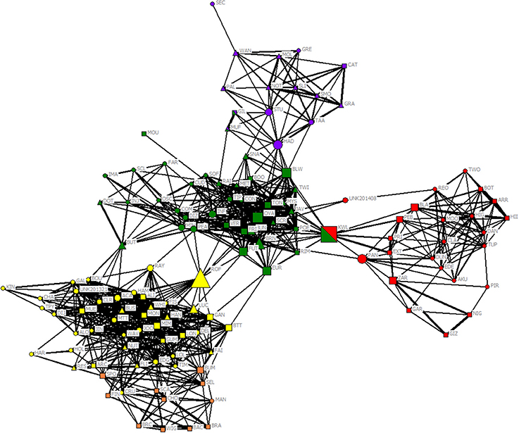
Figure 2. Network diagram for 129 bottlenose dolphins using the HWI. The shape of each node indicates its sex (circle: females; square: males; triangle; unsexed), and the color of each node indicates its unit defined by the modularity of Newman (2006) (purple ComA; red ComB; green ComC; yellow and orange sub-communities D and D'), although three individuals were assigned to two different units depending on the method (Newman vs. Hierarchical linkage). Only links representing affiliations (HWI > 0.16) are shown, and link width is proportional to index weight. Node size is based on the betweenness centrality measure of each individual.

Association Patterns

The overall mean HWI and maximum HWI were 0.05 ± 0.02 (SE) and 0.55 ± 0.19 (SE), respectively. The coefficient of correlation (r) between the true and estimated association indices for the entire study population indicated a moderate representation of the data (r = 0.476 ± 0.024 SE) and a well-differentiated society value (S = 1.020 ± 0.033 SE) suggesting that some individuals form strong associations. We ran this analysis within each community (identified by the network and community analysis) and found values of r higher than 0.4 indicating that our analysis is representative of the true patterns (Table 2).

TABLE 2

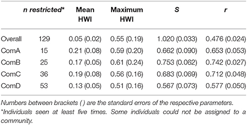
Table 2. The mean association indices for the population overall and per community (ComA, ComB, ComC, and ComD); the measure of social differentiation (S); and the correlation coefficient of the true and estimated association matrices (r).

Tests of preferred/avoided associations showed a significantly higher CV of observed vs. expected association indices (HWI_observed CV = 2.1405, HWI_random CV = 1.8797, P < 0.001) indicating that long-term preferred companions are present in the overall population. The proportion of non-zero association indices was significantly lower in the observed vs. the expected association indices (observed = 0.2648, random = 0.3069, P < 0.001) indicating avoidance between some individuals in the population. More specifically, individuals were more likely to associate with same-sex individuals than among individuals of different sex (Mantel test, HWI_within = 0.07 ± 0.03 SE, HWI_between = 0.05 ± 0.02 SE, P < 0.001), with preferred associations occurring between females (HWI_observed CV = 1.9989, HWI_random CV = 1.7675, P < 0.001), and between males (HWI_observed CV = 2.1770, HWI_random CV = 1.9222, P < 0.0001).

The mean HWI was lower in ComD (0.13 ± 0.05 SE) and higher in ComA (0.21 ± 0.08 SE), although stronger dyads were estimated in ComB (maximum HWI = 0.61 ± 0.24 SE) (Table 2). Mantel test confirmed that associations were stronger within than between communities [HWI_{mean, within} = 0.16 (0.07); HWI_{mean, between} = 0.01 (0.01), P < 0.0001] and individuals were more likely to associate with same-sex individuals than among individuals of different sex in all communities to the exception of ComA (Table 3).

TABLE 3

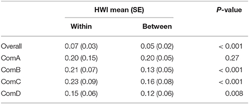
Table 3. Association indices within and among sex classes (Mantel test, 0.05 one-side).

Significant differences between communities were found in the network measures with ComC and ComD communities having higher strength and affinity (Table 4 and see Table S1 in Supplementary Material for Mann-Whitney test, P < 0.02), although the strength was much higher for ComA community when considering all individuals (i.e., including individuals seen less than five times, see Table S2 in Supplementary Material). ComA had the highest clustering coefficient; however, this may be biased by the small number of individuals seen more than five times (n = 15), which may result in individuals appearing more connected than they actually are. ComC had the next highest clustering coefficient, indicating a dense network of individuals in that community.

TABLE 4

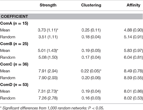
Table 4. Average strength, clustering coefficients, and affinity with comparisons from random calculating using half-weight indices for individuals sighted at least five times.

Preferred associations occurred in all communities with all CVs of association indices higher in the observed vs. the random values (Table 5). Specifically, preferences occurred between females within ComB, ComC, and ComD and between males within ComB and ComD. Although avoidances occurred with the proportions of non-zero indices being lower in the observed vs. the random values, they were not sex-specific in ComC as found in ComD or for males in ComB (Table 5).

TABLE 5

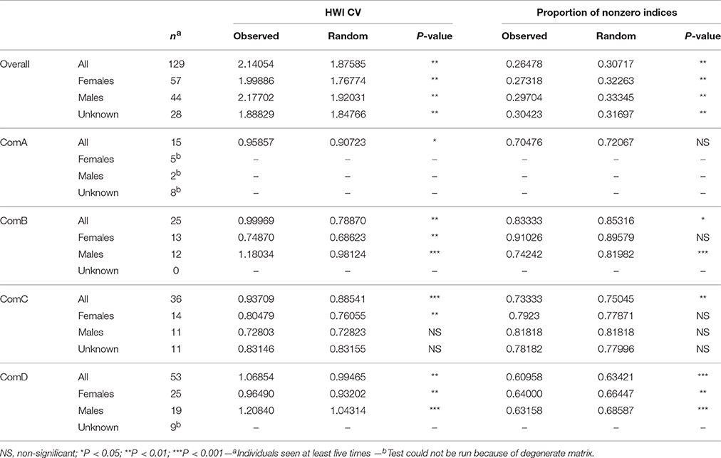
Table 5. Sex class (female, male, unknown sex) permutation tests for preferred (HWI CV) and avoided (proportion of non-zero indices) associations for the population overall and per community.

Lagged association rates (LAR) for each community were higher than the null LARs for the overall population indicating that associations within communities were relatively stable and non-random over the study period (Figure 3). The most parsimonious LAR model (based on the QAICc, Table S3 in Supplementary Material) showed constant companions for all communities and brief associations described as rapid or casual but lasting for less than a day. However, the casual acquaintances in ComB lasted for only a few days.

FIGURE 3

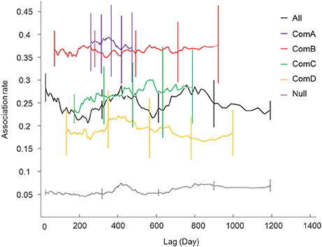
Figure 3. Lagged association rates (LAR) for all individuals (black line) and within the communities (ComA purple; ComB red; ComC green; and ComD yellow). The null association rate (dash lines) and jack-knife error bars are shown.

Female and male LARs (except in ComA) were higher than their respective null LARs, particularly in ComB, indicating that associations between individuals of the same sex were relatively stable over the study period within their respective communities (Figure 4). LARs of males were generally higher than the LARs of females indicating that associations between males were stronger than associations between females, although more females were identified in ComC and ComD (sex ratio 0.71:1 and 0.76:1, respectively). Female and male LARs for ComB were higher than LARs of other communities indicating that associations within ComB were higher than in other communities (this related only to sexed individuals, Figure 4).

FIGURE 4

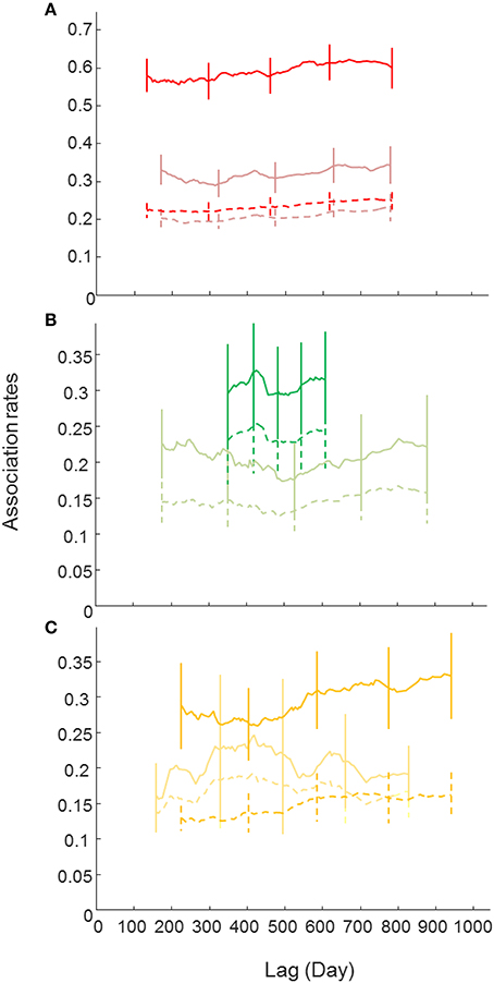
Figure 4. Lagged association rates (LAR) for males and females (bland color) bottlenose dolphins of each community [(A)-ComB, (B)-ComC and (C)-ComD]. The null association rate (dash lines) and jackknife error bars are shown. Note that the LAR for ComA couldn't be estimated because of small sample sizes.

The most parsimonious LAR models (based on the QAICc, Tables S4, S5 in Supplementary Material) for each sex class and per community suggested some long lasting associations and others that were of brief duration because of constant companions and rapid dissociations or casual acquaintances lasting less than a day. However, if not constant, female and male associations in community B still lasted for up to a month or a few days, respectively, before dissociating (Table S4, S5).

Spatial Distribution of Communities

We estimated core areas (50% kernel density) and home ranges (95% kernel density) of each of the four communities using individuals assigned to each respective community. Core areas estimates were similar when using individuals seen at least five times and when including all individuals irrespective of their sighting frequency. Similarly, home range estimates were similar when using individuals seen at least five times and when including all individuals irrespective of their sighting frequency (see Table S6 in Supplementary Material). As such, we have only presented the results using all clustered individuals. The core areas (i.e., 50% kernel density estimated using all individual sightings) of each community were discrete and located in each geographic region (Figure 5A) with sizes varying from 6.83 km² (ComB) to 31.05 km² (ComC) (Table S6). The core area of ComB mainly covered shallow waters (83% coverage at <10 m) while the core area of ComA was mainly in deep water (71% coverage at >10 m) (see Table S7 in Supplementary Material). Home ranges were mainly contained within the respective geographic region (Figure 5B), with the home range of ComB mainly covering the shallow waters of the SCR (61.4% coverage at <10 m). Conversely, the home range of ComA covered much of the GR region, which is mainly deeper waters (55.4% coverage > 15 m). We therefore referred each community to a geographic region, namely ComA to GR; ComB to SCR; ComC to OA, and ComD to CS. Seven individuals (seen less than five times) were not assigned to a community because we could not define the geographic region where they were mainly sighted.

FIGURE 5

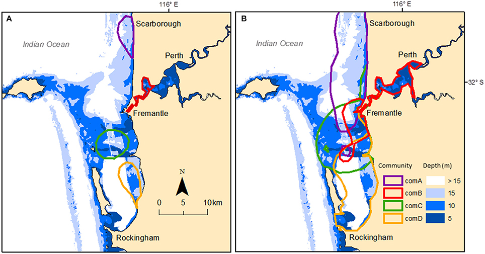
Figure 5. Study area showing the bathymetry and core areas (A) based on the 50% kernel density and home ranges (B) based on the 95% kernel density estimated for each community using clustered individual sightings. Communities are: ComA-purple; ComB-red; ComC-green; and ComD-yellow.

Permutation tests indicated significant avoidance between communities in GR, SCR, and CS, but occurrence of some associations with ComC in OA. However, when tested with all the individuals (including individuals seen less than five times), avoidance tests were all non-significant. There were overlapping home ranges between each of the communities (Figure 5B) with 17% (n = 54 groups) of the groups being composed of individuals from different communities. Most of those multi-community groups (78%) were observed in OA and the lower reach section of SCR (Figure 1B). The smallest home range overlap occurred between ComA and ComD (2.42–7.96 km²) and the largest between ComC and ComD (43.97–45.62 km²) (Table S8 in Supplementary Material). Additionally, 30 and 32% of ComC and ComD home ranges, respectively, overlapped with the core area of ComB, covering the entire Inner Harbor of the Port of Fremantle.

Inspection of the overlap in home ranges for individuals seen at least five times and assigned to a community indicated that there was a clear difference of percentage of overlap from dyads within and between communities, with much higher proportion of dyads sharing >80% of the home range within communities (18, 62, 47, and 36% for ComA, ComB, ComC, and ComD communities, respectively) than between (only 1.1% of the dyads showed that >80% of the home range was shared, although this was not necessarily the case for both individuals of the dyad).

Home range overlap significantly explained the HWI dyads at the population-level (r = 0.10, p < 0.01) and more specifically for dyads allocated to ComA and ComD communities (r_ComA = 0.07, r_ComD = 0.07, p < 0.01). Measures of HWI dyads for individuals allocated to ComB and ComC were not explained by their home range overlap (p > 0.05).

Residence Times

We examined the residency patterns of all individuals (including individuals seen less than five times) per community. Models consisting of parameters indicating the occurrence of emigration and mortality best fitted the LIR of each of the four communities (based on the QAIC, Table S9 in Supplementary Material). Parameters showed differences in community sizes and residency. In ComB, 78% of the individuals were described as residing for nearly 18 years (95% IC: 10–87 years). Conversely, 58% of the individuals observed in ComA were described as individuals staying for maximum of c. five years (95% IC: 3–11 years). Another LIR model represented the demography of ComA best (i.e., emigration, re-immigration, and mortality, ΔQAICc ≤ 2) and showed that a minority of individuals that were considered as a community (n = 20%) also spent more time outside the area than in (Table S9). Most of the individuals in ComC and ComD (n = 63 and 66%, respectively) were described with a long residence, with individuals from ComC staying for 7.5 years (95% IC: 4–23 years) and ComD individuals for about 12 years (95% IC: 7–47 years).

Genetic Relatedness

A total of 107 tissue biopsy samples were collected for genetics analyses. Samples were from individuals identified during the current study and who had been assigned to a community, and were checked for duplicates and removed when allele frequencies were missing for more than four loci. In addition, three loci were removed for further genetic analyses because of scoring errors due to stuttering (SCA27) or because of departure of HWE associated with homozygosity excess (i.e., frequencies of null alleles >0.05 for TexVet5 and SCA17).

We identified 35 pairs of high relatedness values (QG > 0.5), although we did not have prior information on their relatives for most of these. While most pairs (n = 20) were of individuals assigned to the same community, others were identified from individuals assigned to different communities, although no pairs involved individuals from ComA and ComD. The bootstrap values of within-community pairwise genetic relatedness coefficients averaged 0.012 ± 0.005 (95% IC: 0.007, 0.017) over the four communities, whereas the average pairwise genetic relatedness coefficient of the population was −0.008 ± 0.002 (95% IC: −0.011, −0.006). All communities except ComD had positive mean genetic relatedness coefficients (Table 6) and individuals were more related to individuals from the same community than from different communities. However, there were no significant differences in relatedness within and between ComA and ComC (t-test, P-value > 0.05, Table 6). Significant correlation between pairwise relatedness coefficients and HWI was found in ComB (ANOVA, P < 0.05, Table 7), although the correlation was small (R = 0.01).

TABLE 6

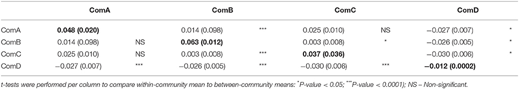
Table 6. Bootstrap mean (and standard error) genetic relatedness (Queller and Goodnight, 1989) for within-community (bold) and with individuals from other communities of bottlenose dolphins (between-community) genotyped with 10 microsatellite loci in Perth metropolitan waters, WA.

TABLE 7

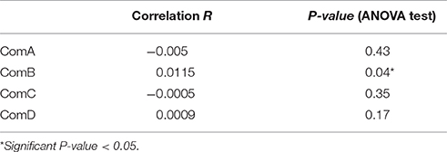
Table 7. Correlation coefficient R and ANOVA test between relatedness coefficient and HWI pairwise within-community.

Discussion

It is imperative to characterize the fine-scale population structure of mobile, continuously distributed species so that an EIA is conducted within an appropriate biological context. The first step in that process is to identify the relevant local wildlife populations that will be affected by a proposed development or activity. Our study demonstrated that social, spatial, ecological, and genetic information may be used to identify local communities of bottlenose dolphins.

Analyses of association patterns of photo-identified bottlenose dolphins revealed four distinct social mixed-sex communities in which patterns of social organization, social dynamics, home ranges, and residency differed (see Table 8 for a summary). Spatial analyses found these communities occupy discrete core areas associated with different environmental and bathymetric characteristics. As expected, high site fidelity and residency patterns were documented for communities occupying shallow, protected embayment and estuary habitats. Overlap in home ranges (e.g., dyads within ComA-GR and ComD-CS) and genetic relatedness (e.g., dyads within SCR community) explained associations between some dyads. However, overall, such factors explained little of the associations between individuals, suggesting that other explanatory factors drive community structure at a local scale.

TABLE 8

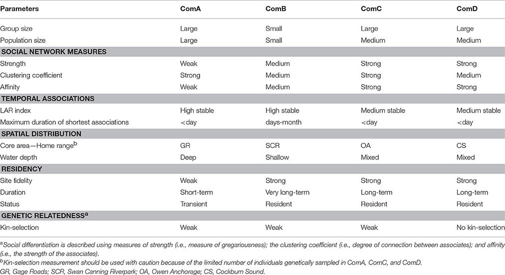
Table 8. Summary comparison of social, temporal, spatial, residency, and genetic patterns across the four communities (ComA, ComB, ComC, and ComD).

Community Segregation

Dolphins exhibited a complex structure of associations across the coastal and estuarine seascape of the study area. Network analysis identified four social mixed-sex communities which have few interactions between them. While some constant companionship relationships were identified in all communities, each community is driven by casual acquaintance relationships demonstrating rapid disassociation and frequent re-association (Wells et al., 1987). However, even for constant companions, the shortest associations between individuals within ComB (i.e., SCR community) lasted for a few days to a month between females, suggesting stronger maternal cooperation (Wells et al., 1987; Lusseau et al., 2003) in the estuary. In fact, the entire ComB (females and males) presented a much higher degree of stability (LAR) than occurred in any of the other communities; this may reflect the ecological constraints associated with estuarine systems (Lusseau et al., 2003) and human pressures.

Social segregation of dolphin populations within nearshore and inshore habitats has been documented in Indo-Pacific bottlenose dolphins elsewhere. For example, discrete communities occur in the Port Stephens embayment in south-eastern Australia, with two communities occupying spatially discrete core areas within the embayment (Wiszniewski et al., 2009). Here, despite some home ranges overlapping (95% KDE), each community was associated with a distinct geographic region within the study area, namely: an estuary (SCR – ComB), a semi-enclosed embayment (OA–ComC and CS–ComD), and an open coastline (GR—ComA). The core areas (50% KDE) of the communities did not overlap, suggesting that ecological differences among communities reflect environmental differences in bathymetry, benthic substrate, and habitat types, as well as human impacts.

Communities also differed in their sociality. Titcomb et al. (2015) demonstrated that habitat shape could have an effect on the structure and association patterns within communities, by influencing movement patterns and encounters between conspecifics. Here, the densest communities in the network, OA (ComC) and CS (ComD) (i.e., indicated by higher strength and affinity), were found in a semi-enclosed embayment. As the SCR community (ComB) occupies an estuary with narrow channels, encounters between conspecifics may occur on a daily basis. However, the mean sociality for that community was not as high, which may reflect the limited number of possible associates given its small size (n = 25, excluding two individuals seen less than five times). Conversely, the GR community (ComA) was the least cohesive, with high redundancy in connection expressed by lower strength, which is consistent with individuals occupying larger ranges and, consequently, less frequent encounters with conspecifics.

The LIR analysis identified clear differences in site fidelity and residency pattern between communities. These differences may be related to the difference in habitat structure and prey distribution between open coastline (GR) and more protected embayment and estuary (OA & CS and SCR) habitats. Individuals in open coastlines often have diminished levels of site fidelity and a more extensive home range (Defran and Weller, 1999; Oudejans et al., 2015; Sprogis et al., 2015). Here, individuals from the GR community (ComA) showed no residency pattern, with most identified individuals seen less than five times and LIR models indicating that individuals spent more time outside the study area. In addition, the large but variable estimates of abundance (Chabanne et al., 2017) suggested that individuals identified in this geographic region (GR) may be members of a larger population located further north. In constrast, residency period was estimated to be more than 7 years in OA and CS and 18 years in SCR, which is consistent with other studies indicating that dolphins occupying shallow and protected areas show a high degree of residency and long-term site fidelity (Wells, 1986; Sprogis et al., 2015; Brusa et al., 2016) and often belong to relatively small and stable communities (Wells et al., 1987). That latter characteristic is consistent with the small size of the resident communities estimated by the LIR model (SCR ≈ 21 residents; OA ≈ 43; and CS ≈ 64) and the abundances estimated via mark-recapture analyses [SCR ≈ 19 individuals and OA/CS (combined) ≈ 122, Chabanne et al., 2017].

While habitat differences seemed to largely account for association differences, range overlap only weakly predicted the association strength of the two communities at the northern and southern extremes (GR and CS). Likewise, genetic relatedness only explained associations within the SCR community. Kin-based and overlapping associations have been recorded in some bottlenose dolphin populations (Parsons et al., 2003; Frère C. H. et al., 2010), but not in others (Möller, 2001). It would therefore appear that other intrinsic or extrinsic factors are likely to drive the social patterns within each community. The KDE method used to calculate the habitat used by each individual is also limited by the sample size (i.e., number of observations per individual). Sprogis et al. (2015), for example, calculated the KDE for individuals seen at least 30 times (Seaman et al., 1999), although other studies indicated that 100–300 observations per individual were necessary to obtain highly precise representation of space use (Girard et al., 2002).

Using Social, Ecological, and Genetic Data to Evaluate the Impact of Developments and Activities on the Relevant Local Population: Four Case Studies

Once the relevant local wildlife populations have been identified, social, spatial, ecological, and genetic information about those local populations can then be used to evaluate potential environmental impacts on those populations. The range of impacts that may affect bottlenose dolphins in coastal and estuarine habitats include: habitat degradation, indirect and direct interactions with commercial and recreational fisheries, vessel disturbance, and environmental contaminants (e.g., Dungan et al., 2012; Pirotta et al., 2013; Todd et al., 2015; Culloch et al., 2016).

To demonstrate the utility of such information for evaluating environmental impacts, we consider four case-study examples of developments or activities that may affect dolphins in the context of one of the local communities identified in this study: pile driving (SCR), dredging of seagrass (OA), operation of a desalination plant (GR), and construction of a large harbor (CS).

Pile Driving in Swan Canning Riverpark (SCR)

Pile driving involves the use of large hammer mounted on a crane to drive piles into the seabed. The process may affect marine mammals by masking underwater sounds, causing behavioral changes (e.g., avoidance), or causing hearing damage or physiological injury (David, 2006; Brandt et al., 2011; Erbe, 2013).

Paiva et al. (2015) observed a decrease in detection of bottlenose dolphins during pile driving activities in the Inner Harbor at Fremantle (located at the entrance to SCR), and suggested that dolphins may have been using other areas during periods of pile driving activity. If such avoidance or displacement behavior occurs, then pile driving may affect dolphins in two relevant ways: (a) a decline or cessation in foraging activity within the harbor, which is a known foraging habitat (Chabanne et al., 2012) and (b) a decline or cessation in the use of the harbor to transit between the estuary and adjacent coastal waters. The latter impact is particularly significant as the harbor is the only access way between the SCR and the adjacent coastal waters. Were movements of dolphins through the harbor to cease or greatly diminish over an extended period of time, then demographic isolation of the SCR community might occur.

Several characteristics of the SCR community make it relatively more vulnerable to long-term demographic isolation and would make local extinction a plausible risk, including: (1) small community size; (2) a recent disease-related mass mortality event (Holyoake et al., 2010); (3) injury and mortality from fishing line entanglement; and (4) exposure to high levels of boat traffic and to occasional harassment.

Dredging in Owen Anchorage (OA)

Dredging of marine habitats may occur to create or maintain infrastructure (e.g., shipping channels) or to remove benthic material such as shellsand for commercial purposes. Todd et al. (2015) reviewed the effects of marine dredging activities on marine mammals and concluded that (a) direct impacts (such as vessel collisions and underwater noise emissions) were unlikely because vessel speeds were slow and (b) the low-frequency levels (below 1 kHz) emitted by dredgers should not cause damage to marine mammal auditory systems. However, underwater noise from dredging may mask prey sounds and dolphin vocalizations and lead to displacement (Pirotta et al., 2013), particularly if activities directly impact on marine mammal prey species (Todd et al., 2015). Dolphins may also be attracted to dredging sites if the disturbance facilitates the capture of fish (e.g., Chilvers and Corkeron, 2001).

A long-term shellsand dredging operation operates in Owen Anchorage which relies on dredging of suitable substrates (Environmental Protection Authority, 2001; BMT Oceania, 2014). The extensive coverage of shallow (<10 m) sand areas and seagrass meadows (BMT Oceania, 2014) sheltered from the oceanic swell in OA means the area is likely to support a broad assemblage of prey species for dolphins (Kendrick et al., 2000; Heithaus and Dill, 2002; Hyndes et al., 2003; Finn, 2005; Sampey et al., 2011). The current management plan for the dredging operation, developed to meet the requirements of approval conditions imposed in 2002 after an EIA of the operation, focuses on the dredging of areas devoid of seagrass to minimize environmental impacts to benthic habitats and fisheries (BMT Oceania, 2014).

The focus on dredging of non-seagrass areas and the overall scale of the dredging operation suggest that impacts on prey availability for dolphins will be localized. Further, impacts from interactions with dredging and transport vessels are unlikely to present a significant risk, as vessel speeds are slow and dolphins do not appear to be attracted to active dredging operations. The OA community identified in this study would be the relevant local population for any EIA of any future proposal to expand the current shellsand dredging operation.

Desalination in Gage Roads (GR)

Impact assessments for the operation of desalination plants in southern Australia have reported low risks of impacts for marine mammals (e.g., Wonthagii, Victoria, Minister for Planning, 2009) (e.g., Cape Riche or Binningup, southern Western Australia, Water Corporation, 2008; Bejder, 2011). However, direct and indirect impacts from brine discharges to the benthic environment (and subsequently to local fauna populations) remain unknown in these areas (Bejder, 2011). In Binningup, for example, prey availability may have been reduced indirectly because of osmoregulation impacts to fish (e.g., cuttlefish, Sepia apama, Dupavillon and Gillanders, 2009; Smith and Sprogis, 2016) or destruction of fish habitats. Such impacts have been reported elsewhere. In Alicante Bay in the northwestern Mediterranean Sea, for example, a seagrass die-off resulted from physiological stress caused by salinity fluctuations associated with brine discharge from two desalination plants (Garrote-Moreno et al., 2014). Physiologically, dolphins and other marine mammals are highly-evolved osmoregulators, with a kidney structure developed for habitats with a broad salinity range, indicating that higher localized salinities should not cause significant physiological stress if exposure to extreme conditions is not prolonged (Ortiz, 2001).

The ecological characteristics of the GR community, principally low site fidelity and more transient behavior, suggest the operation of a proposed desalinization plant in the northern metropolitan waters of Perth (as has been discussed—see Mercer, 2013) would be unlikely to have as adverse an impact as might occur for a community showing strong site fidelity and near continuous occupancy of the affected area. Nonetheless, environmental change may induce displacement (Dungan et al., 2012) or splitting (Nishita et al., 2015) of the community, which may have adverse ecological impacts because some individuals are essential for maintaining the cohesion of the network (i.e., metapopulation) and controlling the flow of information within it (Lusseau and Newman, 2004).

Harbor Construction in Cockburn Sound (CS)

Two harbor developments have been proposed for the Kwinana Shelf region in CS, a private port and a new Outer Harbor facility for the Port of Fremantle. The construction of harbor facilities presents a range of risks for dolphins, including reduction or displacement of dolphins because of direct and indirect impacts from construction-related activities (e.g., Pirotta et al., 2013; Todd et al., 2015; Culloch et al., 2016). Potential impacts on dolphins include but are not limited to: (1) disturbances or changes in behavior from construction noise and vibration; (2) displacement due to a change in prey availability resulting from modification or removal of habitat because of dredging or the construction of infrastructure; and (3) health issues arising from changes in water quality (e.g., sedimentation and increased incidence of algal blooms), circulation patterns (e.g., reduced flushing), and increased chemical contaminants (Environmental Protection Authority, 1998).

Here, the risks of a harbor development are significant because the core area of the CS community is located in the Kwinana Shelf, an area that has ecological significance for dolphins as foraging habitat and as a nursery area (Finn, 2005; Finn and Calver, 2008). In particular, the loss of nursing habitat for females and calves may impose substantial fitness costs on individual dolphins through reduced reproductive success. The strong, long-term spatial association of dolphins with the area and the absence of habitat with environmental characteristics similar to the Kwinana Shelf suggest that dolphins would not be able to compensate for the loss of habitat on the Kwinana Shelf by shifting to other, nearby areas. The extent to which dolphins use new harbor facilities for foraging may depend on the harbor designs, the materials used, and the fish assemblages those areas ultimately sustain.

Conclusions

This study emphasizes the need for EIAs to focus on the relevant local wildlife populations that will be affected by proposed developments and activities. Here, we applied a methodology of broad utility to identify multiple communities of bottlenose dolphins in a heterogeneous coastal environment and then used information on their social and spatial structures, residency patterns, and abundances used to assess the vulnerability of each community to a particular environmental impact. Such results could also be informative for Marine Spatial Planning and Cumulative Impact Mapping. One local population, the SCR community, appeared to be at some risk of local extinction because of its small size and reliance on an estuary which is only connected to adjacent coastal waters by a heavily-used harbor area.

While mobile marine fauna such as bottlenose dolphins may range over large areas of ocean or coastline, they may also exhibit fine-scale population structure reflecting long-term residency, strong site fidelity, limited ranging patterns and strong, long-term associations with particular conspecifics. Other species may exhibit short-term residency in defined coastal areas, e.g., for breeding or feeding. The proper evaluation of impacts of coastal and estuarine developments therefore requires information about the distribution of species at an individual level (i.e., spatial and temporal scales) and their connection at community level (i.e., metapopulation dynamics).

Author Contributions

DC, HF, and LB conceived the study. DC collected, organized, processed, and analyzed the data. LB advised on the analysis. DC wrote the manuscript with contribution to drafting, critical review, and editorial input from HF and LB. All authors critically reviewed the manuscript with final proofs.

Funding

For financial, technical, and logistical support, we thank the Swan River Trust, Fremantle Ports and Fremantle Sailing Club. DC was supported throughout her PhD by an Australian Postgraduate Award, Murdoch University Research Excellence Scholarship and a Murdoch Strategic Top-up.

Conflict of Interest Statement

The authors declare that the research was conducted in the absence of any commercial or financial relationships that could be construed as a potential conflict of interest.

Fremantle Ports and the Swan River Trust provided financial support for this research. While this manuscript does not specifically aim to assess impacts of developments on the dolphin communities, Fremantle Ports and the Swan River Trust have commercial interests (FP) and statutory responsibilities of the assets in the study area. We note that the Swan River Trust has now been amalgamated with the Department of Parks and Wildlife.

Acknowledgments

We thank numerous research assistants who volunteered with fieldwork and data processing. We are grateful to S. Allen for training in biopsy sampling. We thank S. Allen, D. McElligott, and A. Kopps who obtained some of the biopsies and C. Frère for sexing and providing microsatellite loci data for genetic relatedness. We thank the Western Australia Department of Transport for the bathymetry data.

Supplementary Material

The Supplementary Material for this article can be found online at: https://www.frontiersin.org/article/10.3389/fmars.2017.00148/full#supplementary-material

References

Australian Bureau of Statistics (2015). Regional Population Growth, Australia, 2014-15 [Online]. Available online at: http://www.abs.gov.au/ausstats/abs@.nsf/mf/3218.0 (Accessed April 11, 2016).

Barrat, A., Barthelemy, M., Pastor-Satorras, R., and Vespignani, A. (2004). The architecture of complex weighted networks. Proc. Natl. Acad. Sci. U.S.A. 101, 3747–3752. doi: 10.1073/pnas.0400087101

PubMed Abstract | CrossRef Full Text | Google Scholar

Bastos, R., Pinhanços, A., Santos, M., Fernandes, R. F., Vicente, J. R., Morinha, F., et al. (2016). Evaluating the regional cumulative impact of wind farms on birds: how can spatially explicit dynamic modelling improve impact assessments and monitoring? J. Appl. Ecol. 53, 1330–1340. doi: 10.1111/1365-2664.12451

CrossRef Full Text | Google Scholar

Bejder, L. (2011). Appendix: Cape Riche Desalination Plant—Marine Mammal Assessment. Perth, WA.

Bejder, L., Fletchert, D., and Brager, S. (1998). A method for testing association patterns of social animals. Anim. Behav. 56, 719–725. doi: 10.1006/anbe.1998.0802

PubMed Abstract | CrossRef Full Text | Google Scholar

Bejder, L., Hodgson, A. J., Loneragan, N. R., Allen, S. J., and Cagnazzi, D. D. (2012). Coastal dolphins in north-western Australia: the need for re-evaluation of species listings and short-comings in the Environmental Impact Assessment process. Pac. Conserv. Biol. 18, 56–63. doi: 10.1071/PC120022

CrossRef Full Text | Google Scholar

Bejder, L., Samuels, A., Whitehead, H., Finn, H., and Allen, S. (2009). Impact assessment research: use and misuse of habituation, sensitisation and tolerance in describing wildlife responses to anthropogenic stimuli. Mar. Ecol. Prog. Ser. 395, 177–185. doi: 10.3354/meps07979

CrossRef Full Text | Google Scholar

BMT Oceania (2014). Long-Term Shellsand Dredging Owen Anchorage. Dredging and environmental management plan—stage 2 west Success Bank. Perth, WA.

Borgatti, S. P. (2002). NetDraw: Graph Visualization Software. Lexington, KY: Harvard Analytic Technologies.

Brandt, M. J., Diederichs, A., Betke, K., and Nehls, G. (2011). Responses of harbour porpoises to pile driving at the Horns Rev II offshore wind farm in the Danish North Sea. Mar. Ecol. Prog. Ser. 421, 205–216. doi: 10.3354/meps08888

CrossRef Full Text | Google Scholar

Bridge, P. D. (1993). “Classification,” in Biological Data Analysis, eds J. C. Fry (Oxford: Oxford University Press), 219–242.

Brittingham, M. C., Maloney, K. O., Farag, A. M., Harper, D. D., and Bowen, Z. H. (2014). Ecological risks of shale oil and gas development to wildlife, aquatic resources and their habitats. Environ. Sci. Technol. 48, 11034–11047. doi: 10.1021/es5020482

PubMed Abstract | CrossRef Full Text | Google Scholar

Brown, A. M., Bejder, L., Pollock, K. H., and Allen, S. J. (2016). Site-specific assessments of the abundance of three inshore dolphin species to inform conservation and management. Front. Mar. Sci. 3:4. doi: 10.3389/fmars.2016.00004

CrossRef Full Text | Google Scholar

Brown, A. M., Kopps, A. M., Allen, S. J., Bejder, L., Littleford-Colquhoun, B., Parra, G. J., et al. (2014). Population differentiation and hybridisation of Australian snubfin (Orcaella heinsohni) and Indo-Pacific humpback (Sousa chinensis) dolphins in north-western Australia. PLoS ONE 9:e101427. doi: 10.1371/journal.pone.0101427

PubMed Abstract | CrossRef Full Text | Google Scholar

Brusa, J. L., Young, R. F., and Swanson, T. (2016). Abundance, ranging patterns, and social behavior of bottlenose dolphins (Tursiops truncatus) in an estuarine terminus. Aquat. Mamm. 42, 109–121. doi: 10.1578/AM.42.1.2016.109

CrossRef Full Text | Google Scholar

Buchanan, F. C., Friesen, M. K., Littlejohn, R. P., and Clayton, J. W. (1996). Microsatellites from the beluga whale Delphinapterus leucas. Mol. Ecol. 5, 571–575. doi: 10.1046/j.1365-294X.1996.00109.x

PubMed Abstract | CrossRef Full Text | Google Scholar

Burnham, K. P., and Anderson, D. R. (2002). Model Selection and Multimodel Inference: A Practical Information-Theoretic Approach. New York, NY: Springer-Verlag.

Google Scholar

Cagnazzi, D., Parra, G. J., Westley, S., and Harrison, P. L. (2013). At the heart of the industrial boom: australian snubfin dolphins in the Capricorn Coast, Queensland, need urgent conservation action. PLoS ONE 8:e56729. doi: 10.1371/journal.pone.0056729

PubMed Abstract | CrossRef Full Text | Google Scholar

Cairns, S. J., and Schwager, S. J. (1987). A comparison of assocation indices. Anim. Behav. 35, 1454–1469. doi: 10.1016/S0003-3472(87)80018-0

CrossRef Full Text | Google Scholar

Cantor, M., and Whitehead, H. (2013). The interplay between social networks and culture: theoretically and among whales and dolphins. Philos. Trans. R. Soc. B 368:20120340. doi: 10.1098/rstb.2012.0340

PubMed Abstract | CrossRef Full Text | Google Scholar

Cassens, I., Van Waerebeek, K., Best, P. B., Tzika, A., Van Helden, A. L., Crespo, E. A., et al. (2005). Evidence for male dispersal along the coasts but no migration in pelagic waters in dusky dolphins (Lagenorhynchus obscurus). Mol. Ecol. 14, 107–121. doi: 10.1111/j.1365-294X.2004.02407.x

PubMed Abstract | CrossRef Full Text | Google Scholar

Chabanne, D., Finn, H., Salgado-Kent, C., and Bejder, L. (2012). Identification of a resident community of bottlenose dolphins (Tursiops aduncus) in the Swan Canning Riverpark, Western Australia, using behavioural information. Pac. Conserv. Biol. 18, 247–262. doi: 10.1071/PC120247

CrossRef Full Text | Google Scholar

Chabanne, D. B. H., Pollock, K. H., Finn, H., and Bejder, L. (2017). Applying the multistate capture-recapture robust design to assess metapopulation structure of a marine mammal. Methods Ecol. Evol. doi: 10.1111/2041-210X.12792. [Epub ahead of print].

CrossRef Full Text

Chen, L., and Yang, G. (2008). A set of polymorphic dinucleotide and tetranucleotide microsatellite markers for the Indo-Pacific humpback dolphin (Sousa chinensis) and cross-amplification in other cetacean species. Conserv. Genet. 10, 697–700. doi: 10.1007/s10592-008-9618-x

CrossRef Full Text | Google Scholar

Chilvers, B. L., and Corkeron, P. J. (2001). Trawling and bottlenose dolphins' social structure. Proc. R. Soc. Lond. B 268, 1901–1905. doi: 10.1098/rspb.2001.1732

PubMed Abstract | CrossRef Full Text | Google Scholar

Culloch, R. M., Anderwald, P., Brandecker, A., Haberlin, D., McGovern, B., Pinfield, R., et al. (2016). Effect of construction-related activities and vessel traffic on marine mammals. Mar. Ecol. Prog. Ser. 549, 231–242. doi: 10.3354/meps11686

CrossRef Full Text | Google Scholar

David, J. A. (2006). Likely sensitivity of bottlenose dolphins to pile-driving noise. Water Environ. J. 20, 48–54. doi: 10.1111/j.1747-6593.2005.00023.x

CrossRef Full Text | Google Scholar

Defran, R. H., and Weller, D. W. (1999). Occurence, distribution, site fidelity, and school size of bottlenose dolphins (Tursiops truncatus) off San Diego, California. Mar. Mamm. Sci. 15, 366–380. doi: 10.1111/j.1748-7692.1999.tb00807.x

CrossRef Full Text | Google Scholar

DeYoung, R. W. (2007). “Genetics and applied management: using genetic methods to solve emerging wildlife management problems,” in Wildlife Science—Linking Ecological Theory and Management Applications, eds T. E. Fulbright and D. G. Hewitt (Broken Sound Parkway, NW: CRC Press), 317–336.

Google Scholar

Dungan, S. Z., Hung, S. K., Wang, J. Y., and White, B. N. (2012). Two social communities in the Pearl River Estuary population of Indo-Pacific humpback dolphins (Sousa chinensis). Can. J. Zool. 90, 1031–1043. doi: 10.1139/Z2012-071

CrossRef Full Text | Google Scholar

Dupavillon, J. L., and Gillanders, B. M. (2009). Impacts of seawater desalination on the giant Australian cuttlefish Sepia apama in the upper Spencer Gulf, South Australia. Mar. Environ. Res. 67, 207–218. doi: 10.1016/j.marenvres.2009.02.002

PubMed Abstract | CrossRef Full Text | Google Scholar

Efron, B., and Stein, C. (1981). The jackknife estimate of variance. Ann. Stat. 9, 586–596. doi: 10.1214/aos/1176345462

CrossRef Full Text | Google Scholar

Elliott, M., and Whitfield, A. K. (2011). Challenging paradigms in estuarine ecology and management estuarine. Estuar. Coast. Shelf Sci. 94, 306–314. doi: 10.1016/j.ecss.2011.06.016

CrossRef Full Text | Google Scholar

Environmental Protection Authority (1998). The Marine Environment of Cockburn Sound—Strategic Environmental Advice. Perth, WA.

Environmental Protection Authority (2001). Long-Term Shellsand Dredging, Owen Anchorage, Cockburn Cement Ltd. (Report and recommendations of the Environmental Protection Authority). Perth, WA.

Erbe, C. (2013). International regulation of underwater noise. Acoust. Aust. 41, 12–19.

Google Scholar

Finn, H. (2005). Conservation Biology of Bottlenose Dolphins (Tursiops sp.) in Perth Metropolitan Waters. PhD thesis, Murdoch University, Perth, WA.

Finn, H., and Calver, M. C. (2008). Feeding aggregations of bottlenose dolphins and seabirds in Cockburn Sound, Western Australia. West. Aust. Nat. 26, 157–172.

Google Scholar

Fox, A. D., Desholm, M., Kahlert, J., Christensen, T. K., and Krag Petersen, I. B. (2006). Information needs to support environmental impact assessment of the effects of European marine offshore wind farms on birds. Ibis 148, 129–144. doi: 10.1111/j.1474-919X.2006.00510.x

CrossRef Full Text | Google Scholar

Frère, C. H. H., Krützen, M., Mann, J., Watson-Capps, J. J. J., Tsai, Y. J. J., Patterson, E. M., et al. (2010). Home range overlap, matrilineal and biparental kinship drive female associations in bottlenose dolphins. Anim. Behav. 80, 481–486. doi: 10.1016/j.anbehav.2010.06.007

CrossRef Full Text | Google Scholar

Frère, C. H., Krzyszczyk, E., Patterson, E. M., Hunter, S., Ginsburg, A., and Mann, J. (2010). Thar she blows! A novel method for DNA collection from cetacean blow. PLoS ONE 5:e12299. doi: 10.1371/journal.pone.0012299

PubMed Abstract | CrossRef Full Text | Google Scholar

Garrote-Moreno, A., Fernandez-Torquemada, Y., and Sanchez-Lizaso, J. L. (2014). Salinity fluctuation of the brine discharge affects growth and survival of the seagrass Cymodocea nodosa. Mar. Pollut. Bull. 81, 61–68. doi: 10.1016/j.marpolbul.2014.02.019

PubMed Abstract | CrossRef Full Text | Google Scholar

Gilson, A., Syvanen, M., Levine, K., and Banks, J. (1998). Deer gender determination by polymerase chain reaction: validation study and application to tissues, bloodstains, and hair forensic samples from California. Calif. Fish Game 84, 159–169.

Google Scholar

Girard, I., Ouellet, J.-P., Courtois, R., Dussault, C., and Breton, L. (2002). Effects of sampling effort based on GPS telemetry on home-range size estimations. J. Wildl. Manag. 66, 1290–1300. doi: 10.2307/3802962

CrossRef Full Text | Google Scholar

Glasson, J., Thrivel, R., and Chadwick, A. (2012). Introduction to Environmental Impact Assessement. New York, NY: Routledge.

Google Scholar

Heithaus, M. R., and Dill, L. M. (2002). Food availability and tiger shark predation risk influence bottlenose dolphin habitat use. Ecology 83, 480–491. doi: 10.2307/2680029

CrossRef Full Text | Google Scholar

Hill, D., Hockin, D., Price, D., Tucker, G., Morris, R., and Treweek, J. (1997). Bird disturbance: improving the quality and utility of disturbance research. J. Appl. Ecol. 34, 275–288. doi: 10.2307/2404876

CrossRef Full Text | Google Scholar

Holyoake, C., Finn, H., Stephens, N., Duignan, P., Salgado, C., Smith, H., et al. (2010). Technical Report on the Bottlenose Dolphin (Tursiops aduncus) Unusual Mortality Event within the Swan Canning Riverpark, June-October 2009. Perth, WA.

Google Scholar

Hyndes, G. A., Kendrick, A. J., MacArthur, L. D., and Stewart, E. (2003). Differences in the species- and size-composition of fish assemblages in three distinct seagrass habitats with differing plant and meadow structure. Mar. Biol. 142, 1195–1206. doi: 10.1007/s00227-003-1010-2

CrossRef Full Text | Google Scholar

Jefferson, T. A., Hung, S. K., and Würsig, B. (2009). Protecting small cetaceans from coastal development: impact assessment and mitigation experience in Hong Kong. Mar. Policy 33, 305–311. doi: 10.1016/j.marpol.2008.07.011

CrossRef Full Text | Google Scholar

Kearse, M., Moir, R., Wilson, A., Stones-Havas, S., Cheung, M., Sturrock, S., et al. (2012). Geneious basic: an integrated and extendable desktop software platform for the organization and analysis of sequence data. Bioinformatics 28, 1647–1649. doi: 10.1093/bioinformatics/bts199

PubMed Abstract | CrossRef Full Text | Google Scholar

Kendrick, G. A., Hegge, B. J., Wyllie, A., Davidson, A., and Lord, D. A. (2000). Changes in seagrass cover on Success and Parmelia Banks, Western Australia between 1965 and 1995. Estuar. Coast. Shelf Sci. 50, 341–353. doi: 10.1006/ecss.1999.0569

CrossRef Full Text | Google Scholar

Krützen, M., Barre, L. M., Moller, L. M., Heithaus, M. R., Simms, C., and Sherwin, W. B. (2002). A biopsy system for small cetaceans: darting success and wound healing in Tursiops spp. Mar. Mamm. Sci. 18, 863–878. doi: 10.1111/j.1748-7692.2002.tb01078.x

CrossRef Full Text | Google Scholar

Levins, R. (1969). Some demographic and genetic consequences of environmental heterogeneity for biological control. Am. Entomol. 15, 237–240. doi: 10.1093/besa/15.3.237

CrossRef Full Text | Google Scholar

Lusseau, D., and Newman, M. E. J. (2004). Identifying the role that animals play in their social networks. Proc. R. Soc. Lond. B 271, S477–S481. doi: 10.1098/rsbl.2004.0225

PubMed Abstract | CrossRef Full Text | Google Scholar

Lusseau, D., Schneider, K., Boisseau, O. J., Haase, P., Solooten, E., Dawson, S. M., et al. (2003). The bottlenose dolphin community of Doubtful Sound features a large proportion of long-lasting associations. Behav. Ecol. Sociobiol. 54, 396–405. doi: 10.1007/s00265-003-0651-y

CrossRef Full Text | Google Scholar

MacLeod, C. D. (2014). An Introduction to Using GIS in Marine Biology. Supplementary workbook four. Investigating home ranges of individual animals. Glasgow: Pictish Beast Publications.

Google Scholar

Mann, J., Connor, R. C., Barre, L. M., and Heithaus, M. R. (2000). Female reproductive success in bottlenose dolphins (Tursiops sp.): life history, habitat, provisioning, and group-size effects. Behav. Ecol. 11, 210–219. doi: 10.1093/beheco/11.2.210

CrossRef Full Text | Google Scholar

McCluskey, S. M., Bejder, L., and Loneragan, N. R. (2016). Dolphin prey availability and calorific value in an estuarine and coastal environment. Front. Mar. Sci. 3:30. doi: 10.3389/fmars.2016.00030

CrossRef Full Text | Google Scholar

Mercer, D. (2013). Dry Climate Limits Water Options. The West Australian.

Minister for Planning (2009). Victoria Desalination Project Assessment under Environment Effects Act 1978.

Moilanen, A., and Nieminen, M. (2002). Simple connectivity measures in spatial ecology. Ecology 84, 1131–1145. doi: 10.2307/3071919

CrossRef Full Text | Google Scholar

Möller, L. M. (2001). Social Organisation and Genetic Relationships of Coastal Botlenose Dolphins in Southeastern Australia. PhD thesis, Macquarie University.

Morrison, M. L., Marcot, B. G., and Mannan, R. W. (2006). Wildlife-Habitat Relationship: Concepts and Applications. Washington, DC: Isanld Press.

Google Scholar

Newman, M. E. J. (2004). Analysis of weighted networks. Phys. Rev. 70:056131. doi: 10.1103/PhysRevE.70.056131

PubMed Abstract | CrossRef Full Text | Google Scholar

Newman, M. E. J. (2006). Modularity and community structure in networks. Proc. Natl. Acad. Sci. U.S.A. 103, 8577–8582. doi: 10.1073/pnas.0601602103

PubMed Abstract | CrossRef Full Text | Google Scholar

Nishita, M., Shirakihara, M., and Amano, M. (2015). A community split among dolphins: the effect of social relationships on the membership of new communities. Sci. Rep. 5:17266. doi: 10.1038/srep17266

PubMed Abstract | CrossRef Full Text | Google Scholar

Ortiz, R. M. (2001). Review - Osmoregulation in marine mammals. J. Exp. Biol. 204, 1831–1844.

PubMed Abstract | Google Scholar

Oudejans, M. G., Visser, F., Englund, A., Rogan, E., and Ingram, S. N. (2015). Evidence for distinct coastal and offshore communities of bottlenose dolphins in the North East Atlantic. PLoS ONE 10:e0122668. doi: 10.1371/journal.pone.0122668

PubMed Abstract | CrossRef Full Text | Google Scholar

Paiva, E. G., Salgado Kent, C. P., Gagnon, M. M., McCauley, R., and Finn, H. (2015). Reduced detection of Indo-Pacific bottlenose dolphins (Tursiops aduncus) in an Inner Harbour channel during pile driving activities. Aquat. Mamm. 41, 455–468. doi: 10.1578/AM.41.4.2015.455

CrossRef Full Text | Google Scholar

Parsons, K. M., Durban, J. W., Claridge, D. E., Balcomb, K. C., Noble, L. R., and Thompson, P. M. (2003). Kinship as a basis for alliance formation between male bottlenose dolphins, Tursiops truncatus, in the Bahamas. Anim. Behav. 66, 185–194. doi: 10.1006/anbe.2003.2186

CrossRef Full Text | Google Scholar

Pirotta, E., Laesser, B. E., Hardaker, A., Riddoch, N., Marcoux, M., and Lusseau, D. (2013). Dredging displaces bottlenose dolphins from an urbanised foraging patch. Mar. Pollut. Bull. 74, 396–402. doi: 10.1016/j.marpolbul.2013.06.020

PubMed Abstract | CrossRef Full Text | Google Scholar

Queller, D. C., and Goodnight, K. F. (1989). Estimating relatedness using genetic markers. Evolution 43, 258–275. doi: 10.2307/2409206

CrossRef Full Text | Google Scholar

Quintana-Rizzo, E., and Wells, R. S. (2001). Resighting and association patterns of bottlenose dolphins (Tursiops truncatus) in the Cedar Keys, Florida: insights into social organization. Can. J. Zool. 79, 447–456. doi: 10.1139/z00-223

CrossRef Full Text | Google Scholar

Rice, W. R. (1989). Analyzing tables of statistical tests. Evolution 43, 223–225. doi: 10.2307/2409177

CrossRef Full Text | Google Scholar

Rooney, A. P., Merritt, D. B., and Derr, J. N. (1999). Microsatellite diversity in captive bottlenose dolphins (Tursiops truncatus). J. Hered. 90, 228–253.

PubMed Abstract | Google Scholar

Rousset, F. (2008). GENEPOP'007: a complete re-implementation of the genepop software for Windows and Linux. Mol. Ecol. Resour. 8, 103–106. doi: 10.1111/j.1471-8286.2007.01931.x

PubMed Abstract | CrossRef Full Text | Google Scholar

Salgado Kent, C., McCauley, R. D., Parnum, I. M., Gavrilov, A. N., Kent, C. P. S., and Gavrilov, N. (2012). Underwater noise sources in Fremantle inner harbour: dolphins, pile driving and traffic. Acoust. Aust. 1–7.

Google Scholar

Sampey, A., Fromont, J., and Johnston, D. J. (2011). Demersal and epibenthic fauna in a temperate marine embayment, Cockburn Sound, Western Australia: determination of key indicator species. J. R. Soc. West. Aust. 94, 1–18.

Google Scholar

Sandoval-Castillo, J., and Beheregaray, L. B. (2015). Metapopulation structure informs conservation management in a heavily exploited coastal shark (Mustelus henlei). Mar. Ecol. Prog. Ser. 533, 191–203. doi: 10.3354/meps11395

CrossRef Full Text | Google Scholar

Schnell, G. D., Watt, D. J., and Douglas, M. E. (1985). Statistical comparison of proximity matrices: applications in animal behaviour. Anim. Behav. 33, 239–253. doi: 10.1016/S0003-3472(85)80138-X

CrossRef Full Text | Google Scholar

Seaman, D. E., Millspaugh, J. J., Kernohan, B. J., Brundige, G. C., Raedeke, K. J., and Gitzen, R. A. (1999). Effects of sample size on kernel home range estimates. J. Wildl. Manag. 63, 739–747. doi: 10.2307/3802664

CrossRef Full Text | Google Scholar

Silva, M. A., Prieto, R., Magalhães, S., Seabra, M. I., Santos, R. S., and Hammond, P. S. (2008). Ranging patterns of bottlenose dolphins living in oceanic waters: implications for population structure. Mar. Biol. 156, 179–192. doi: 10.1007/s00227-008-1075-z

CrossRef Full Text | Google Scholar

Smith, H. C., and Sprogis, K. R. (2016). Seasonal feeding on giant cuttlefish (Sepia apama) by Indo-Pacific bottlenose dolphins (Tursiops aduncus) in south-western Australia. Aust. J. Zool. 64, 8–13. doi: 10.1071/ZO15075

CrossRef Full Text | Google Scholar

Smolker, R. A., Richards, A. F., Connor, R. C., and Pepper, J. W. (1992). Sex differences in patterns of association among Indian Ocean bottlenose dolphins. Behaviour 123, 38–69.

Google Scholar

Sprogis, K. R., Raudino, H. C., Rankin, R., MacLeod, C. D., and Bejder, L. (2015). Home range size of adult Indo-Pacific bottlenose dolphins (Tursiops aduncus) in a coastal and estuarine system is habitat and sex-specific. Mar. Mamm. Sci. 32, 287–308. doi: 10.1111/mms.12260

CrossRef Full Text | Google Scholar

Steidl, R. J., and Powell, B. F. (2006). Asessing the effects of human activities on wildlife. GW Forum 23, 50–58.

Google Scholar

Sweanor, L. L., Logan, K. A., and Hornocker, M. G. (2000). Cougar disperal patterns, metapopultion dynamics, and conservation. Conserv. Biol. 14, 798–808. doi: 10.1046/j.1523-1739.2000.99079.x

CrossRef Full Text | Google Scholar

Thomas, L., Laake, J. L., Rexstad, E., Strindberg, S., Marques, F. F. C., Buckland, S. T., et al. (2009). Distance 6.0. release 1. Research Unit for Wildlife Population Assessment, University of St. Andrews.

Titcomb, E. M., O'Corry-Crowe, G., Hartel, E. F., and Mazzoil, M. S. (2015). Social communities and spatiotemporal dynamics of association patterns in estuarine bottlenose dolphins. Mar. Mamm. Sci. 31, 1314–1337. doi: 10.1111/mms.12222

CrossRef Full Text | Google Scholar

Todd, V. L. G., Todd, I. B., Gardiner, J. C., Morrin, E. C. N., MacPherson, N. A., DiMarzio, N. A., et al. (2015). A review of impacts of marine dredging activities on marine mammals. ICES J. Mar. Sci. 72, 328–340. doi: 10.1093/icesjms/fsu187

CrossRef Full Text | Google Scholar

Torres, A., Jaeger, J. A. G., and Alonso, J. C. (2016). Assessing large-scale wildlife responses to human infrastucture development. Proc. Natl. Acad. Sci. U.S.A. 113, 8472–8477. doi: 10.1073/pnas.1522488113

PubMed Abstract | CrossRef Full Text | Google Scholar

Van Oosterhout, C., Hutchinson, W. F., Wills, D. P. M., and Shipley, P. (2004). Micro-Checker: software for identifying and correcting genotyping errors in microsatellite data. Mol. Ecol. Notes 4, 535–538. doi: 10.1111/j.1471-8286.2004.00684.x

CrossRef Full Text | Google Scholar

Walker, F. M., Sunnucks, P., and Taylor, A. C. (2008). Evidence for habitat fragmentation altering within-population processes in wombats. Mol. Ecol. 17, 1674–1684. doi: 10.1111/j.1365-294X.2008.03701.x

PubMed Abstract | CrossRef Full Text | Google Scholar

Wang, J. (2011). COANCESTRY: a program for simulating, estimating and analysing relatedness and inbreeding coefficients. Mol. Ecol. Resour. 11, 141–145. doi: 10.1111/j.1755-0998.2010.02885.x

PubMed Abstract | CrossRef Full Text | Google Scholar

Waples, R. S. (1998). Separating the wheat from the chaff: patterns of genetic differentiation in high gene flow species. J. Hered. 89, 438–450. doi: 10.1093/jhered/89.5.438

CrossRef Full Text | Google Scholar

Water Corporation (2008). Southern Seawater Desalination Project. Report and recommendations of the Environmental Protection Authority. Perth, WA.

Wells, R. S. (1986). Population Structure of Bottlenose Dolphins: Behavioral Studies of Bottlenose Dolphins along the Central West Coast of Florida. Contract Report to National Marine Fisheries Service; Southeast Fisheries Center, (NMFS, SEFSC). Miami, FL.

Wells, R. S., Boness, D. J., and Rathbun, G. B. (1999). “Behavior,” in Biology of Marine Mammals, eds J. E. Reynolds and S. A. Rommel (Washington, WC; London: Smithsonian Institution Press), 324–422.

Google Scholar

Wells, R. S., Scott, M. D., Irvine, A. B., and Genoways, H. (1987). “The social structure of free-ranging bottlenose dolphins,” in Current Mammalogy, ed H. H. Genoways (New York, NY: Plenum), 247–305.

Google Scholar

Western Australian Planning Commission (2004). Fremantle Ports Outer Harbour Project - Information Brochure. Perth, WA.

Whitehead, H. (1995). Investigating structure and temporal scale in social organizations using identified individuals. Behav. Ecol. 6, 199–208. doi: 10.1093/beheco/6.2.199

CrossRef Full Text | Google Scholar

Whitehead, H. (1999). Testing association patterns of social animals. Anim. Behav. 57, F26–F29. doi: 10.1006/anbe.1999.1099

PubMed Abstract | CrossRef Full Text | Google Scholar

Whitehead, H. (2001). Analysis of animal movement using opportunistic individual-identifications: application to sperm whales. Ecology 82, 1417–1432. doi: 10.2307/2679999

CrossRef Full Text | Google Scholar

Whitehead, H. (2007). Selection of models of lagged identification rates and lagged association rates using AIC and QAIC. Commun. Stat. Simul C 36, 1233–1246. doi: 10.1080/03610910701569531

CrossRef Full Text | Google Scholar

Whitehead, H. (2008a). Analyzing Animal Societies: Quantitative Methods for Vertebrate Social Analysis. Chicago, IL: Chicago University Press.

Google Scholar

Whitehead, H. (2008b). Precision and power in the analysis of social structure using associations. Anim. Behav. 75, 1093–1099. doi: 10.1016/j.anbehav.2007.08.022

CrossRef Full Text | Google Scholar

Whitehead, H. (2009). SOCPROG programs: analysing animal social structures. Behav. Ecol. Sociobiol. 63, 765–778. doi: 10.1007/s00265-008-0697-y

CrossRef Full Text | Google Scholar

Whitehead, H. (2016). SOCPROG: Programs for Analyzing Social Structure. Nova Scotia, CA: Dalhousie University.

Google Scholar

Whitehead, H., Bejder, L., and Ottensmeyer, A. (2005). Testing association patterns: issues arising and extensions. Anim. Behav. 69, e1–e6. doi: 10.1016/j.anbehav.2004.11.004

CrossRef Full Text

Wiszniewski, J., Allen, S. J., and Moller, L. M. (2009). Social cohesion in a hierarchically structured embayment population of Indo-Pacific bottlenose dolphins. Anim. Behav. 77, 1449–1457. doi: 10.1016/j.anbehav.2009.02.025

CrossRef Full Text | Google Scholar

Würsig, B., and Jefferson, T. A. (1990). Methods of photo-identification for small cetaceans. Rep. Int. Whal. Commn. 12, 43–52.

Google Scholar