Simplifying Regional Tuning of MODIS Algorithms for Monitoring Chlorophyll-a in Coastal Waters

Introduction

Chlorophyll-a (chl-a) concentrations provide a valuable measure of phytoplankton biomass in the marine environment. Phytoplankton biomass can provide an indicator of trophic state in marine systems due to an association with anthropogenic nutrient pressures (Smith et al., 1999). Consequently chl-a is commonly monitored, particularly in coastal marine environments, as part of a wider suite of indicators (Bricker et al., 2003; Giovanardi and Vollenweider, 2004). However, field monitoring and analysis of chl-a is a resource-intensive process which may limit the temporal and spatial coverage of monitoring by relevant authorities.

A traditional way of monitoring chl-a in aquatic systems involves field analysis of in situ chl-a fluorescence. For logistical reasons, field sampling is often unable to match the spatial and temporal scale of variability in phytoplankton biomass. Since the launch of ocean-color sensors such as the Coastal Zone Color Scanner (CZCS) in the 1970s, multispectral and hyperspectral satellite remote sensing data are routinely processed to estimate oceanic water chl-a concentrations. Many satellite sensors are currently available to monitor chl-a, making them potentially useful tools for management, but the use of the data in coastal waters requires local calibration and validation (IOCCG, 2000).

The rewards from successful satellite algorithm development for coastal waters are high. For example the MODIS (Moderate Resolution Imaging Spectroradiometer) Aqua and Terra satellite datasets have been collected daily from 1999, with some of these data easily viewable through webtools such as Worldview (https://worldview.earthdata.nasa.gov/) and CawthronEye (http://www.cawthron.org.nz/apps/cawthroneye). Consequently there is the potential to access over a decade of twice daily surface data at a spatial resolution of about 1 km². As well as the MODIS datasets, there are several other accessible satellite datasets. The MERIS (MEdium Resolution Imaging Spectrometer) instrument offered additional insights due to a greater number of spectral bands, and provides a template for the Ocean Land Color Imager (OLCI) launched on Sentinel-3. However, MERIS is not currently operational and so it has limited opportunities for calibration to contemporary datasets. Similarly the LandSat satellites also offer high spatial resolution (30 m), but have a limited number of relevant spectral bands for aquatic research and only a 16-day temporal resolution. Consequently we selected MODIS satellite data for use in this study.

In order to quantify radiance across many spectral bands, the receiving satellite sensor relies on sunlight penetrating the atmosphere and the surface ocean water. The incident light will be affected by various factors in the water that interfere and change the intensity of light of different wavelengths that arrive at the satellite sensor. These factors include absorbance by waterborne constituents and atmospheric aerosols and can include other factors such as ocean surface waves or bottom reflectance. It is these spectral modifications that can affect the estimation of properties, such as chl-a concentrations in surface waters.

Accurate estimation of chl-a concentration, from satellite-sensed data cannot be tested and validated without substantial field datasets, which equates to a large effort for an unknown result. This is particularly true for chl-a in optically complex coastal waters. The common issue to overcome is the overlap in the spectral response with other water constituents such as colored dissolved organic matter (CDOM; IOCCG, 2000). Internationally, freely accessible satellite-derived chl-a data in coastal waters are increasingly being used with newly developed algorithms. However, little application of satellite data to New Zealand coastal waters has occurred, with only a limited number of studies undertaken for coastal monitoring (Jones et al., 2013). We suspect the limited uptake may be associated with the risk of unsuccessful results and lack of access to tools and advice to assist with calibration of satellite data algorithms for estimating chl-a in coastal waters. Indeed a recent survey study by Schaeffer et al. (2013) identified a number of factors that limit the use of satellite data globally.

Many algorithms have been developed for estimating chl-a from MODIS and SeaWiFS (Sea viewing Wide Field-of-view Sensor) data, ranging from empirical to more physically realistic “semi-empirical” algorithm approaches. Examples of commonly used global empirical algorithms are: the OC3M algorithm (Carder et al., 2004) for MODIS, the OC2 and OC4 algorithms for SeaWiFS, and the OC4Me for MERIS (O'Reilly et al., 1998, 2000; Morel et al., 2007). These algorithms have been routinely used to process satellite images for oceanic (referred to here as Case 1) waters (IOCCG, 2000), where phytoplankton and their derivatives predominantly determine the optical properties (Morel, 1988). For most coastal and inland (Case 2) waters, where sediments or dissolved yellow substance make an important or dominant contribution to the optical properties (Morel, 1988), the algorithms may fail to produce accurate estimates (Ruddick et al., 2000; Moses et al., 2009). For more reliable estimates of chl-a concentrations, the application of algorithms to Case 2 waters will need to be locally validated (Kahru et al., 2014).

The present study explores the potential usage of readily accessible MODIS multispectral data for describing chl-a variability in coastal waters of New Zealand at two locations (Hawke Bay and Tasman Bay; Figure 1). The study relies on long-term near surface data collected using morred sensors to determine in situ conditions and to investigate the suitability of these data for satellite algorithm development in New Zealand.

FIGURE 1

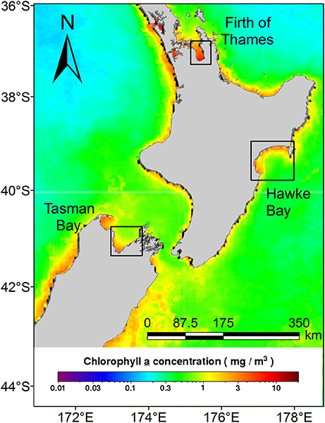
Figure 1. The two New Zealand coastal regions (Tasman and Hawke bays) that are the focus of the study are shown in the two southern boxes with an additional Firth of Thames region (northern-most box) which is discussed, but which is not analyzed in detail here. Mean annual global chlorophyll-a concentrations from the Case 1 OC3M algorithm are shown for 2012. Chlorophyll-a data were sourced at a spatial resolution of 4 km (level 3 data) from the Ocean Color website (https://oceancolor.gsfc.nasa.gov/).

Materials and Methods

Satellite Data

The present study uses MODIS Aqua Level 2 (L2) data, which can be downloaded on request from the OceanColor website (NASA, 2013). Although MODIS Terra data products were also available for this study, these were excluded from our analysis due to identified issues with the data collected by this instrument (Franz et al., 2007). MODIS Level 2 data products have a spatial resolution of about 1 km² and are atmospherically corrected using the standard Near-Infrared (NIR) algorithm for oceanic (Case 1) waters (Gordon and Wang, 1994). For turbid coastal waters, the water-leaving radiance in the near-infrared bands is significantly greater than zero due to suspended particles. Applying the default atmospheric correction algorithm can therefore lead to over-correction of the reflectance and result in negative values for some pixels. Alternative algorithms of atmospheric correction of Case 2 waters can improve radiance reflectance accuracy in turbid coastal waters. For example, using the assumption of negligible water-leaving reflectance in the near-infrared region of the spectrum (Bailey et al., 2010). However, this procedure would require additional processing of less refined Level 1 (L1) data (Aiken and Moore, 1997; Ruddick et al., 2000; Wang and Shi, 2007). Because of aims of this study to consider accessible methods that will improve accessibility of data, additional atmospheric processing of L1 data has not been undertaken for this study.

The L2 data quality was checked before use by inspection of the provided quality flags for atmosphere, land, glint and cloud (specific flags used were: ATMFAIL, LAND, HIGLINT, HILT, CLDICE, CHLFAIL, and ATMWARN). Any flagged data were excluded from future analysis and remaining remote sensing reflectance data with negative values were excluded from the subsequent analyses.

Level 2 processed data files were sourced from the OceanColor website and also included chl-a estimates based on a global OC3M algorithm (Carder et al., 2004; NASA, 2013). The global OC3M chl-a algorithm (Default OC3M) was developed for Case 1 waters and were used for comparison with locally calibrated chl-a algorithms (Local OC3M) developed in this study.

Field Data

Two locations around New Zealand, Tasman Bay and Hawke Bay (Figure 1), were assessed using available water quality data. Several sources of time-series data from moored sensors, and data from discrete water sampling were used to locally calibrate and assess the performance of satellite data algorithms.

In Tasman Bay, a 2 year dataset (April 2011 to March 2013) was available through sensors attached to a moored monitoring buoy named TASCAM (41.058°S 173.091°E, Figure 2). The TASCAM monitoring buoy contained a fluorescent chl-a sensor (Weblabs Eco-FLNTUS), which uses a 470/695 nm excitation-emission frequency to characterize the fluorescent signal with a stated chl-a sensitivity of 0.025 mg/m³. Two chl-a sensors were used over the 2 year deployment period. Both sensors were initially calibrated at the factory (www.wetlabs.com) on the 2nd of August 2010 at an ambient temperature of 22.3°C and were deployed from new to the TASCAM site. The second sensor replaced the initial sensor deployment and was deployed in April 2012. Both sensors were deployed at a depth of 8 m and contained an integrated copper anti-fouling Bio-wiper™ which was closed when no measurements were being taken to prevent fouling. Antifouling was used on the sensor housings, with in situ diver cleaning occurring approximately every 3 months at the site. A 60 min sampling interval was used over the deployment period, with a single fluorescent measurement reported.

FIGURE 2

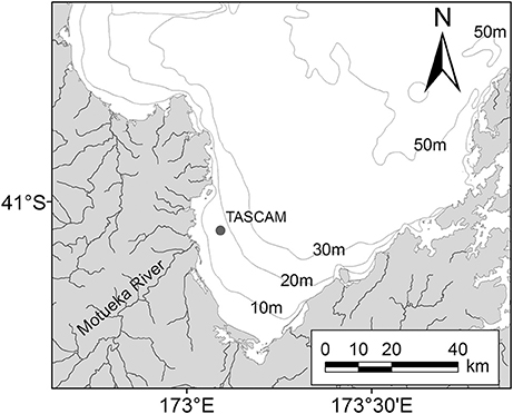
Figure 2. Map showing the location of the TASCAM (dot) monitoring buoy in Tasman Bay and the Motueka River to the south-east of the buoy. Bathymetric depth contours also shown (gray lines).

Hawke Bay chl-a data was accessed from another moored bouy, HAWQi (Hawke Bay water quality information), (39.386°S 176.949°E, Figure 3). This bouy was identical to TASCAM and used the same chl-a sensor (i.e., a WETLabs Eco-FLNTUS with an integrated anti-fouling Bio-wiper™). The chl-a sensor was also deployed from new with factory calibration and cleaned with approximately three-monthly visits to the site. A single sensor at the HAWQi buoy was deployed at a depth of 5 m. Both 30 and 60 min sampling intervals were used over the period December 2012–October 2013, with a single florescent measurement reported. Field accuracy of the chl-a sensor was checked by comparing in situ readings to Van Dorn collected seawater samples from near to the sensor. Processing of in situ samples for chl-a concentrations were obtained following the procedures specified by Lorenzen (1967).

FIGURE 3

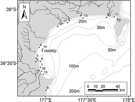
Figure 3. Moored data site of the Hawke Bay water quality information monitoring buoy (HAWQi; +), and State of the Environment (SOE; dots) water sampled sites (3–18) used in this study. Bathymetric depth contours also shown (gray lines).

Chlorophyll-a sampling for the period 2002–2013 from a number of other locations was also collated for Hawke Bay. These data were collected by the Hawke's Bay Regional Council using individual laboratory-analyzed water samples (Figure 3). Due to issues associated with a coarse temporal sampling scale of the data and the proximity of the sampling sites to the coast, these data were excluded from model training. The data were instead used to assess the skill of the algorithm for different areas of the bay to assess the applicability of the algorithm for wider use.

To ensure data from the moored sensors were compatible with the 1 km² resolution satellite data, temporal smoothing using a centered 6 h window moving box mean was applied to both the reported TASCAM and HAWQi buoy data. In the case of the TASCAM data, this equated to a moving box window of six data points. For the higher temporal resolution sampling in the HAWQi time series (i.e., 30 min sampling), 12 data points were averaged. The smoothing over a 6 h time window was undertaken to approximate the 1 km² scale of satellite estimates by accounting for water moving past the moored sensor. The chosen temporal widths equate to movement of 1 km for an average water movement speed of about 4.6 cm/s.

A 6 h time window for both the Tasman and Hawke bays' buoy data balanced the need for spatial smoothing, whilst ensuring that the time period was not too long (i.e., greater than a day). It was recognized that growth or grazing factors could significantly influence the measurements if longer averaging periods were used. Comparison with a progressive vector showed the 6 h window was appropriate for the Tasman Bay site (Figure 4). Comparison to current data for the Hawke Bay site was not possible due to a current meter failure at the site, but mean depth averaged current speeds of 5.6 cm/s observed at a nearby site (39.319°S, 177.090°E) over a 3 month period imply the selected 6 h window was appropriate (Cawthron unpublished data).

FIGURE 4

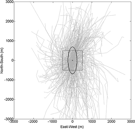
Figure 4. Progressive vectors (light gray) showing estimated surface advection length-scales over a 6 h periods at the TASCAM mooring site. Note the ellipse shows mean advection distances over 6 h and the thin black square shows the 1 km² resolution of satellite data used in the study.

While it is more common to use stringent quasi-simultaneous and spatially collocated match-ups (Gordon and Wang, 1994; Moses et al., 2009; Kahru et al., 2014) to increase the availability of data for comparison, those methods can end up excluding a large fraction of the data for comparison. This can be due to issues such as cloud cover and adjacency to land (Kahru et al., 2014). This approach can also introduce some bias if large gradients exist over small spatial scales (i.e., at or less than the satellite sensor resolution) and there exists a risk that in situ measurements may be matched to optically different water than was sampled (Moses et al., 2009). Because moored sensors allow continuous sampling, our approach aimed to reduce the variability that exists between in situ point-scale measurements and 1 km² satellite retrievals.

In order to prepare in situ samples for the smoothed model development, a nearest temporal match of the closest satellite data product pixel was undertaken to the mean sample time. Typically this time difference was <1 h between the observed chl-a satellite remote sensing time and the smoothed sensor time. But allowance was made for time differences of <3 h either side of a satellite observation to increase the availability of data from the model for construction and testing. This is consistent with time differences from other studies (Gordon and Wang, 1994; Moses et al., 2009; Kahru et al., 2014). As a check of the smoothed-data approach, the single closest-time datum was also used to train separate models for comparison. However, it is important to note that each of the closest-time and smoothed models are predicting different parameters, specifically point-in-time chl-a and smoothed chl-a, respectively.

Models applied in the present study used two empirical approaches for fitting satellite remote sensing reflectance data to observed chl-a concentrations. These models were, a linear model, based on the OC3M algorithm (hereafter: Local OC3M), and a novel non-linear exponential model (hereafter: Exponential) developed for this study.

The Local OC3M takes the form of:

$\begin{array}{l}{log}_{10}(chla)=a_0+a_1.R+a_2.R^2+a_3.R^3+a_4.R^4\end{array}$

Where R = log₁₀(max(Rrs443, Rrs488)/Rrs555), and Rrs443, Rrs488 and Rrs555 refer to remote sensing reflectance at the wavebands centered on 443, 488, and 555 nm, respectively. Model coefficients are defined as a0 to a4 in the equation.

The model coefficients were fitted to both closest-time chl-a and 6 h mean (smoothed) chl-a data and the corresponding satellite remote sensing reflectance ratios (R) using the generalized least-squares linear model fitting routine (glm) from the R software package (R Core Team, 2014).

The remote sensing reflectance ratio, R, of the max(Rrs443, Rrs488) to Rrs555 provides a ratio of light at the peak blue (i.e., 443 nm) chl-a absorbance to a minimum chl-a absorbance (555 nm). Unabsorbed light can be reflected, contributing to the remote reflectance signal, therefore chl-a concentrations are expected to decrease under increasing R (i.e., less 443 nm light is absorbed and more is reflected, relative to 555 nm light). However, phytoplankton specific absorbance is also known to decrease non-linearly (through a power relationship) with increasing chl-a (Bricaud et al., 1995). In order to capture this non-linearity, a simple exponential model was also tested against the data. This exponential model takes the form:

$\begin{array}{l}chla=a{e}^{-kS}\end{array}$

where a and k are model coefficients and S = 10^R. R is the same as defined in the OC3M linear modeling approach, so S = max(Rrs443, Rrs488)/Rrs555. In formulating S, we chose to remove the logarithm from R, as it is redundant in an exponential model. Furthermore, as S will always be positive (provided negative Rrs values are removed) this insures that chl-a estimates cannot be less than zero, which is a benefit over the OC 4th order polynomial approach.

Coefficients for the Exponential model were fit to both the closest-time chl-a and 6 h mean chl-a data and the corresponding satellite remote sensing reflectance ratios (S). Model fitting was undertaken using the non-linear least squares (nls) model fitting routine from the R software package (R Core Team, 2014). In the case of the Tasman Bay data, a limited range to the chl-a data was observed over the sampling period (maximum chl-a = 2.76 mg/m³). This was a value that is lower than the observed range of chl-a values in the region which have been noted to be up to about 10 mg/m³ (MacKenzie and Gillespie, 1986). As the coefficient, a, in the model provides a constraint on the maximum predictable order to allow for model fitting to higher values in the case of Tasman Bay a fixed value of 10 was also selected for the coefficient a to allow prediction of maximum observed values.

For all model constructions, each dataset was split into two parts, where two-thirds of the data were randomly selected for model training and the remaining one-third was used for evaluation of model performance (i.e., “test” data). Although the initial derivation of the data split was random, the same division of the data were used for both the closest-time and smoothed data models to allow comparative performance to be assessed.

The accuracy of different models was assessed using several measures used in other remote sensing (IOCCG, 2006; Moore et al., 2009) and modeling studies (Zhang et al., 2010). Calculation of the regression parameters for the observed vs. derived data (i.e., slope and intercept), the deviance explained (r square), the root mean square error (RMSE) and the average absolute percentage error (ε) were reported for the smoothed data, with a subset, deviance explained and RMSE only calculated for closest match data.

The relevant calculations for RMSE and average absolute percentage error (ε) are specified here:

$\begin{array}{l}RMSE=\sqrt{\frac{1}{n}{\displaystyle \sum }{\left[\mathrm{\text{lo}}{\mathrm{\text{g}}}_{10}(chl{a}_{observed})-\mathrm{\text{lo}}{\mathrm{\text{g}}}_{10}(chl{a}_{derived})\right]}^2}\\ \epsilon =\frac{1}{n}{\displaystyle \sum }\frac{|chl{a}_{derived}-chl{a}_{observed}|}{chl{a}_{observed}}\times 100\end{array}$

where n is sample size.

Another measure, the relative central frequency (RCF), which reports the proportion of percentage error that lies within ± 50% of observed values, is also calculated (Zhang et al., 2010). All analyses were conducted using the R software package (R Core Team, 2014).

Results

Results of model training to 6 h averaged and closest-time matchups are both presented here, along with their performance information within their respective regions. Overview statistics for the chl-a datasets from the two regions are presented in Table 1.

TABLE 1

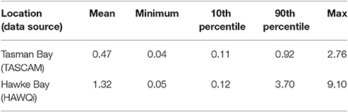
Table 1. Statistics for the two chlorophyll-a datasets (mg/m³) used for algorithm development.

Six-Hour Mean Models

Tasman Bay

After matching TASCAM chl-a data with the corresponding satellite remote sensing reflectance data, a total of 394 data points were available. The two models (Local OC3M and Exponential) were then trained on the random two-thirds of the total dataset. TASCAM chl-a data were used as the dependent variable and the ratios of satellite remote sensing reflectance (R) as independent variables. Table 2 provides the summary of the output of the two models.

TABLE 2

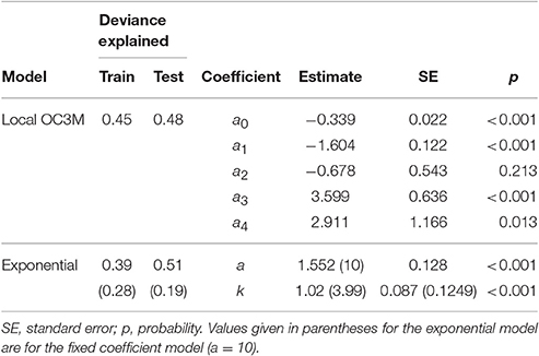
Table 2. Summary of results of the two locally-tuned models for Tasman Bay trained on 6 h averaged data.

Validation using the remaining one-third of the data showed that both locally fitted models performed better than the global Case 1 OC3M (Default OC3M) model (Figure 5). The two local models displayed significant improvement over the global OC3M algorithm in all performance measures used (Table 3). For example, deviance explained increased from 0.09 for the global algorithm to 0.49 and 0.52 for the local models. The RMSE decreased from 0.71 for the global algorithm to ~0.22 and 0.24 for the local algorithms. The average percentage error decreased significantly from 465% for the global algorithm, to 48 and ~56% for the two local algorithms (Table 3).

FIGURE 5

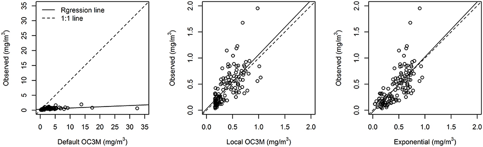
Figure 5. Default (global Case 1) and local model predictions vs. 6-h averaged in situ TASCAM monitoring buoy chlorophyll-a test dataset for the three different model approaches in Tasman Bay. Note that a different scale is used for the global Default OC3M model results.

TABLE 3

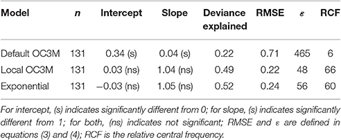
Table 3. Comparison of accuracy of the default (global Case 1) and local model predictions using the TASCAM monitoring buoy test dataset; n = sample size and significance test results are shown in brackets.

Comparison of predicted chl-a with field data (Figure 6) shows that, though the model can underestimate the peaks, it generally follows time series and therefore may be useful in monitoring trends in the coastal water environments of the bay. Despite the long period of deployment for the sensors at the TASCAM site, no clear drift in sensor response was apparent over the deployment period (Figure 6).

FIGURE 6

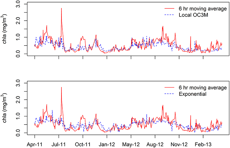
Figure 6. Comparison of the 6 h averaged TASCAM monitoring buoy data with model predicted chlorophyll-a (chla) using Local OC3M (upper) and Exponential model (lower).

Hawke Bay

A total of 174 data points were used for training and testing of the satellite models. Two-thirds of the dataset (N = 114) was used for model construction, and the remaining one-third (N = 58) for the evaluation model performance. The model summary is given in Table 4.

TABLE 4

Table 4. Summary of the locally-tuned model outputs for the Hawke Bay water quality information (HAWQi) monitoring buoy for the 6 h averaged data.

Model validation using the remaining one third of the HAWQi dataset shows that both local algorithms performed better than the global OC3M model (Figure 7). Typically, the two models achieved significantly higher deviance explained, lower percent error (ε) and RMSE (Table 5). For example, the average percentage error for the local OC3M model reached 32%, which is within an acceptable upper limit of 35% (IOCCG, 2006; Moore et al., 2009). Although the exponential algorithm produced a higher average percentage error (47%) than the local OC3M model, the exponential model exhibited less bias when compared to in situ data from the test dataset (Figure 7, Table 5).

FIGURE 7

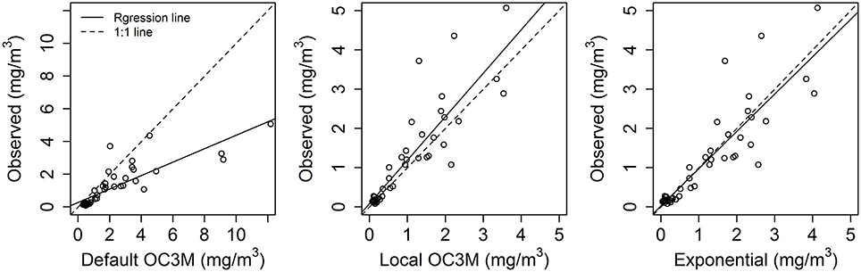
Figure 7. Default (global Case 1) and local model predictions vs. 6 h averaged in situ HAWQi (Hawke Bay water quality information monitoring buoy) chlorophyll-a concentrations using test dataset for the three different model approaches. Note that a different scale is used for the global Default OC3M results.

TABLE 5

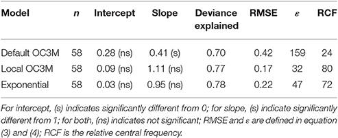
Table 5. Comparison of accuracy of the default (global Case 1) and local model predictions using the Hawke Bay water quality information monitoring buoy (HAWQi) test dataset; n = sample size and significance test results are shown in brackets.

Comparison of the predicted time series with HAWQi buoy data also shows that both the local models performed reasonably well (Figure 8). The modeled chl-a was able to track observed trends in the buoy data for most of the time series, with the exception of a short period in September 2013 (Figure 8). Similarly in situ seawater sample results taken beside the sensor were generally comparable to the mooring sensor result, highlighting the accuracy of the sensor over the deployment period (Figure 8).

FIGURE 8

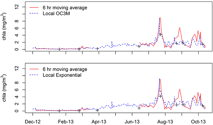
Figure 8. Comparison of 6 h averaged HAWQi data with predicted chlorophyll-a (chla) concentrations using Local OC3M model (upper) and Exponential model (lower). Also shown is the field sampled data (+) collected from beside the chlorophyll-a sensor at the site.

When applied to other areas of the bay using additional water sample data from the region, the algorithms did not compare well with the collected data at most sites (Figure 9, Table 6). Although the two local algorithms performed better than the global OC3M algorithm, there was a high average percentage error (Figure 9, Table 6).

FIGURE 9

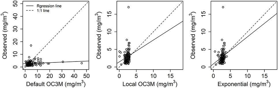
Figure 9. Default (global Case 1) and local model predictions vs. 6 h averaged in situ State of the Environment (SOE) chlorophyll-a concentrations for the three different model approaches. Note: the different scale for the global OC3M comparison.

TABLE 6

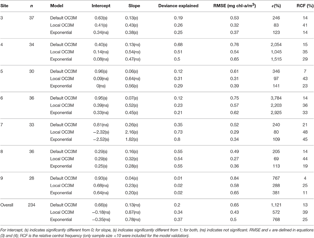
Table 6. Model comparison with Hawke Bay water sample data; n = sample size and significance test results are shown in brackets.

Closest-Time Models

Tasman Bay

Using the closest match data to train the two local models produced different coefficients to the models built using smoothed data (Table 7). The model performance on the test data was also decreased when compared to the smoothed data models. Specifically, deviance explained decreased from 0.48 to 0.26 for the OC3M model and from 0.51 to 0.41 for the Exponential model (Tables 2, 7). These results were mirrored in the RMSE results, which also showed increases from 0.23 to 0.34 for the OC3M model and from 0.24 to 0.28 for the Exponential model (Table 3).

TABLE 7

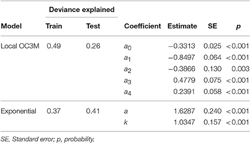
Table 7. Summary of results of the two locally-tuned models for Tasman Bay trained on closest-time data.

Hawke Bay

Using the closest match data also produced different coefficients to the models built using smoothed data at the Hawke Bay site (Table 8). However, at this site, the model performance decline on the test data was generally less pronounced than the smoothed data models. Specifically, deviance explained decreased from 0.75 to 0.28 for the OC3M model and from 0.51 to 0.41 for the Exponential model (Tables 4, 8). The decrease in performance was more pronounced in the RMSE results, which also showed error increases from 0.17 to 0.58 for the OC3M model and 0.22 to 0.60 for the Exponential model (Table 5).

TABLE 8

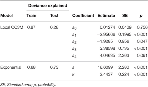
Table 8. Summary of locally-tuned model output for the HAWQi monitoring buoy trained on closest-time data.

Discussion

The present study compared estimates of chl-a concentrations from freely available ocean color data (MODIS Aqua Level 2) with long-term field measurements. The study shows that the standard global OC3M algorithm over-estimated chl-a concentrations at all coastal study sites. The average percentage error ranged between 150 and ~500%. This is in agreement with previous findings that showed that the chl-a retrievals from standard Case 1 MODIS algorithms typically over-estimate chl-a concentration for turbid coastal waters (Darecki and Stramski, 2004; Magnuson et al., 2004; Werdell et al., 2009). Although the global Case 1 OC3M algorithm typically over-estimated chl-a concentration for coastal waters in our study, it appears that aspects of the model may still be useful in coastal environments provided the model is locally tuned.

In the case of the two locations analyzed for this study, there were potentially different optical regimes in place based on the composition of the respective catchments that drain into these locations. In the case of Tasman Bay, the site is located about 8 km from the mouth of the Motueka River (Figure 2). This river drains a catchment with a large proportion of native vegetation cover and subsequently high inputs of colored dissolved organic material which may affect the optical properties of the site. The catchments around the Hawke Bay site are largely associated with pastoral farming and the HAWQi buoy was located further away from major rivers, consequently differing signal to noise ratios in the chl-a response to incoming solar radiation were likely.

Modeling Approaches

Differing coefficients were observed in each model formulation, which is due in part to both optical differences inherent at the two sites, and the range of observed chl-a at each site. The local OC3M model may provide a preferred approach based on its historical use and because this model generally achieved lower average percentage error (ε) than the exponential model (Tables 2, 4, 5). However, the exponential model better captured the deviance in the observations of chl-a based on a higher deviance explained values (Tables 2, 4, 5). Such contradictions based on different measures, shows the need for the use of several measures to evaluate model performance and careful selection based on relevant scientific, or management, objectives for the data. For example, a bias error could have greater impacts on long-term trend analysis.

While the simple exponential model applied in this study does not have the historical use of the OC3M approach, it is clear that it has a similar performance and there are fewer degrees of freedom. The reduced flexibility for fitting the exponential model implies that it would be less likely to result in statistical over-fitting of the model. This is consistent with the results presented here, which show that deviance explained for the exponential model is higher in both test dataset results (i.e., Tables 2, 4) and with the results of the comparison with independent datasets. Given the similar performance of the empirical approaches across the two case studies presented, we consider that local calibration of the exponential model is potentially a more robust approach to construction of empirical locally calibrated chl-a models. As indicated by the results of a naïve fitting of the exponential model to the Tasman Bay data, clearly any model needs to be checked for its relevance to the region of interest. In the case of the Tasman Bay, the Exponential model will only able to estimate chl-a concentrations up to 1.55 mg /m³ (i.e., the a coefficient value), this is limited when compared to measured historical maxima of 10 mg chl-a/m³ (MacKenzie and Gillespie, 1986).

Fitting using an informed coefficient may be one way to avoid this issue; however comparison of the two exponential models constructed for Tasman Bay shows a coincident reduction in the deviance explained by a second model which used a fixed coefficient (Table 2). Consequently, this method may be appropriate for producing a useful model in the absence of representative data, but should ideally be updated as more representative data become available. Setting a bounded maximum in the model also further reduces the degrees of freedom for the fitting process, potentially further reducing over-fitting. While a value of 10 mg chl-a/m³ has been used in Tasman Bay, it is possible that higher concentrations could also have occurred but have not been recorded. Therefore, the use of predetermined fixed coefficients appropriate to the environments of the models (e.g., oligiotrophic coastal temperate, eutrophic coastal tropical environments etc.) could be considered. For example, the Hawkes Bay Exponential model also has an artificial limit (14.79 mg chl-a/m³; Table 4); while this is a reasonable limit for this region, the model will not be able to resolve higher concentrations. Therefore, pre-classification of the environment and the use of an appropriate coefficient for the environment under consideration may be a worthwhile undertaking. The use of predetermined coefficients has the potential to introduce some bias to the tuning process, but the incorporation of this prior knowledge could also yield some benefits to the models. Consequently, while it is worthy of future research, it is not possible to recommend this approach at this time.

The Effect of Spatial Smoothing on Model Training

Despite the issues noted in the modeling of the Tasman Bay site, the results of the effects of smoothing were consistently better across both models and sites. Improved model fit to test data was seen at the TASCAM and HAWQi sites, with better performance observed in both the RMSE and deviance explained performance measures. However, the effect differed at the two sites, suggesting that the benefits may vary. For this reason we would recommend training both smoothed and closest-time models and selecting the best performing model against independent data.

Accuracy of the Models

In considering the measured performance of the algorithms against in situ sensor data, it is important to recognize that the fluorescence data are themselves an estimate of the “true” chl-a concentrations at the sites. The sensors in this study were factory calibrated and new at the time of deployment and we saw no evidence of issues that can affect the accuracy of in situ fluorometric sensors (e.g., quenching, fouling etc.). However, the quality of these underlying data is critical and the differences in the resulting parameterization of the models suggests that there are optical differences between sites. This does not appear to have affected our results (and we aim to study the underlying optical regimes in more detail in future), but we offer this modeling approach as a first step to allow naïve tuning of readily available satellite data to existing datasets.

The accuracy of the local models in the present study significantly improved on the results of the standard Case 1 OC3M algorithm, particularly in the case of Tasman and Hawke bays. In Hawke Bay, the Local OC3M algorithm achieved an average error of 32%. This is within the lower limit for the margin of error set by NASA for retrieving chl-a of within 35% accuracy for the global open oceans (Hooker et al., 1992; Le et al., 2013). The Hawke Bay water sample dataset comparison showed average errors in the range of 40–60%, but were of limited use due to reasons stated previously (e.g., turbid near shore locations, point-in-time samples). Despite the issues, it was interesting to see that the model estimates for some of the Hawke Bay sites (e.g., sites 7 and 8; Table 6) still compared well to data. These results are comparable to the accuracy achieved in other studies for turbid waters (Le et al., 2013) and better than those reported by Shang et al. (2014), where the average percent errors from locally-tuned algorithms were typically in the range of 60–130%. Consequently, the algorithms developed for the HAWQi site presented in this study can be considered satisfactory for future use. Although the Exponential model for the TASCAM site achieved a satisfactory error metric, unfortunately a lack of representative data from a wide range of conditions means that the model is likely only to be accurate for low chl-a conditions. While we have only presented results from two sites, the algorithm fitting approaches presented here will be useful for other coastal water investigations.

The modeling approach presented here (i.e., Tasman Bay and Hawke Bay) generally performed well at the locations and data they were tuned to, but the application of the approach to another region located in the North of New Zealand (the Firth of Thames; Figure 1) was not successful. The Firth of Thames is a similar environment to the Tasman and Hawke bays, but the main difference was that Firth of Thames chl-a data was provided from 15 m vertically-integrated seawater samples taken at fortnightly and monthly frequencies (Jones et al., 2013). Despite a lack of high temporal resolution fluorometric data, available data for the Firth of Thames were plentiful and were comprised of lab analyzed water samples for the period 2002 to 2013, which equated to about 1,300 samples across five sites. The results of Firth of Thames are not presented here, but we note that the results of a similar study (Jones et al., 2013) yielded a model with a low deviance explained (0.15).

We consider a likely explanation for the difficulty in training accurate models at the Firth of Thames site was the lack of higher frequency data available at that time. The field data for Tasman and Hawke bays were collected continuously at least every hour and could therefore either be smoothed to approximate the spatial resolution of the satellite (i.e., 1 km²), or closely matched in time. This was not possible with the data available in the Firth of Thames. In this regard, it appears continuous buoy data can facilitate local satellite algorithm development, ideally with lab-processed data used to check sensor accuracy. The difficulty of matching in-water data to satellite observations in dynamic coastal regions has been extensively discussed (e.g., Gordon and Wang, 1994), with issues arising from both temporal matchups and spatial variability at a subpixel (<300 m) level. While temporal smoothing, or closer time matching, of the buoy data does not solve all of these issues, it may help to match spatial and temporal variability in regions where more restrictive criteria (Bailey and Werdell, 2006; Kahru et al., 2014) would limit potential matchups.

Uptake of Satellite Data in the New Zealand Context

Several factors may have prevented wider application of the freely accessible satellite data for coastal waters around New Zealand. While chl-a data for Case 1 coastal waters are readily available, our research shows these are not applicable to the Case 2 coastal waters around New Zealand without additional tuning. Several specific Case 2 algorithms have been developed for other studies that have successfully improved chl-a data retrieval for coastal waters (Ahn and Shanmugam, 2006; Cannizzaro and Carder, 2006; Shanmugam, 2011; Simon and Shanmugam, 2012; Le et al., 2013). While these models were successful, they are regionally specific and may be complex to calibrate locally without specialist equipment and additional targeted studies. Consequently we propose alternate methods that may allow use of existing long-term datasets to begin to unlock previously under-utilized historical data from satellites.

Development of generalized algorithms applicable for coastal waters in different regions requires not only an understanding of the optical properties of phytoplankton, but also other particles and dissolved material. This can be problematic, as it may involve greater resource requirements; e.g., collection of concurrent in situ measurements of pigment concentration and radiometric reflectance (IOCCG, 2000). As a result, the potentially invaluable information provided by satellite reflectance has not been widely utilized in New Zealand to date. It also seems that this is a wider issue than just New Zealand, as recognized by Schaeffer et al. (2013) who note that more effort is required to ensure that managers are aware of the value in the data, and that real and perceived hurdles need to be overcome to improve the uptake of remotely sensed data.

Our study provides evidence of some successful outcomes based on two case studies in New Zealand and that local calibration of empirical chl-a algorithms from pre-processed L2 data products is feasible in New Zealand coastal waters. It also shows that these locally calibrated algorithms may be validated in new regions with optically different properties. Furthermore, the methods we have employed can be achieved using readily accessible techniques and freely available software reducing barriers to the use of the data.

Local calibration of chl-a model in coastal environments may be more likely to succeed if the following recommendations are considered:

• If possible, use high temporal resolution data (at least hourly) to improve the availability of data for model training.

• In situ data should be collected across all seasons (i.e., a year) to ensure a wide range of local optical conditions are observed for model building.

• In situ collection depths are important, because satellite sensors only provide optical information from surface waters. Where coastal waters are turbid and stratified, measurements will need to be close to the surface, but if possible multiple depths should be collected to assess vertical variability.

• Bottom reflections in shallow water have the potential to complicate algorithm development. Similar issues may also occur in turbid waters, with Raman scattering of about 8% previously reported (Gupta, 2015). For this reason data collection for algorithm development should be carried out in optically deep waters (i.e., low reflection and scattering) if possible.

• Empirical fitting of the OC3M algorithm may be prone to over-fitting when compared to a simpler exponential model presented in this study. This could limit its use outside of the training period and location; consequently testing on a leave-out (or “test”) or completely independent dataset is highly recommended.

• The use of the simple exponential model approach is recommended given it generally performed better than a locally calibrated OC3M algorithm with the same data.

• Even if a reasonable level of fit is achieved to reflectance ratio data, assess the utility of the model for estimating the full range of conditions in the region should be assessed, not just the period of data for which the model was trained.

• If high temporal resolution data are available, consider averaging the data to match the spatial-scales for model building and compare to a closest-time approach. While our results differed between sites and the model applied, smoothing generally improved our models when compared to independent data.

Future Implications

Successful calibration of satellite data over ~1 year potentially offers access to over a decade of data at daily (or more frequent) temporal resolution. Using the methods presented here, long-term trends in chl-a concentrations can be interrogated at sites that have perhaps been poorly sampled in the past. Because chl-a is a common indicator of primary production and symptoms of eutrophication, this information can then provide important insights into coastal health.

In the case of New Zealand, expansion of land-based farming is leading to large changes in the flow of nutrients to coastal environments (e.g., Heggie and Savage, 2009). These new pressures have the potential to affect the health of downstream coastal waters, but historical environment monitoring records are limited in their spatial and temporal extent. In order to allow for improved planning decisions on land and in the sea, long-term reliable datasets at many locations will be required to ensure that trends can be detected early and managed appropriately. Consequently remotely-sensed satellite data will play an increasingly important role in providing ongoing information on the state of surface waters for New Zealand. The initial studies presented here highlight that existing field datasets may be able to help assist in unlocking satellite data for such purposes. However, ideally empirical modeling methods (such those presented here) should be continued to be improved upon, as resources and data become available. This will ensure that modeled datasets are robust outside of both the times and areas that they are tuned for.

Conclusions

Simplified methods for regional tuning of satellite algorithms that can produce comparable water quality results to in situ samples are required to improve the uptake of satellite data for coastal monitoring. This study presents results from the local calibration and validation of two empirical algorithm approaches for chl-a, including a simple exponential model developed for this study. There appear to be benefits from the novel method of training the models to spatially-matched data scales, which suggests this approach is worth considering if the available data are appropriate for this purpose. Key to this approach is the use of high-frequency data from moored sensors, which can help to overcome issues with match-up limitations that have previously documented in highly dynamic coastal regions (Gordon and Wang, 1994; Kahru et al., 2014).

Good performance of a simple empirical model trained from high frequency data from moored sensors and standard satellite reflectance products illustrates that local calibration and operational use of readily available satellite data products for coastal waters is feasible. Further research and data collection will be required to more fully validate the methods presented in this study, but we note that pragmatic advice to assist in the application and use of satellite data in coastal waters is currently limited which could restrict the uptake of these valuable datasets. While successful calibration cannot always be guaranteed for satellite datasets, we have identified simple steps that appear to improve model performance.

Author Contributions

WJ undertook the majority of statistical analysis of this work, the production of figures and initially suggested the use of simpler models for development in this project consequently his efforts have been recognized with primary authorship for this paper. Recent health issues have limited WJ's recent involvement in this work, nevertheless he has read and accepted this submission. BK has undertaken the majority of the writing for this manuscript and has helped guide the development of the work undertaken in the study. CC has contributed to sections in this submission and acted in an oversight role. PB was responsible for the data collection used in this study and the methods associated with this submission. The efforts of RK have mirrored that of CC and he has brought an large amount background knowledge to this study. Early versions of this manuscript also drew on RK's extensive knowledge of US datasets with which model were tested against truly independent datasets. Although these data were ultimately removed, they helped provide all authors with additional confidence to progress with publishing this work and represent a significant contribution.

Funding

Cawthron Institute Internal Investment Fund (Grant Number 15954) provided the majority of funding for this work.

Conflict of Interest Statement

The authors declare that the research was conducted in the absence of any commercial or financial relationships that could be construed as a potential conflict of interest.

Acknowledgments

NASA and the team at the Ocean Biology Processing Group (OBPG) are thanked for the provision of the MODIS satellite data used in this study and the tools used to acquire these data. Kent Headley, Paul Cohen, and the rest of the team at the Monterey Bay Aquarium Research Institute are thanked for their time and assistance in developing the technology used in the TASCAM and HAWQi buoy platforms. Waikato Regional Council, particularly Hilke Giles and the late Vernon Pickett are thanked for their support of the initial research that was applied to the Firth of Thames in which many of the methods developed in this paper where initially established. The Hawke's Bay Regional Council, particularly Oliver Wade and Anna Madarasz-Smith are thanked for the timely provision of data and support in the initial HAWQi model development. The Ministry for Business Innovation and Employment Envirolink programme provided support for aspects of the Hawke Bay research (Grant number: 1436-HBRC199). We wish to thank the Wilsons Bay Area A Consortium for their provision of data used in Jones et al. (2013), while these data are not presented in this study it proved helpful for identifying the shortcomings of coarse temporal measurements in satellite model development. Preparation of this paper was supported by the Cawthron Institute Internal Investment Fund and the Ministry of Business Innovation & Employment Catalyst Leaders Fund (Grant number: ILF-CAW1601). Lastly we would like to thank Dr Paul Gillespie and Gretchen Rasch for their valuable comments on the drafts of this paper, and the efforts of peer reviewers and editorial staff that have contributed to this publication.

References

Ahn, Y. H., and Shanmugam, P. (2006). Detecting the red tide blooms from satellite ocean color observations in optically complex Northeast—Asia Coastal waters. Remote Sens. Environ. 103, 419–437. doi: 10.1016/j.rse.2006.04.007

CrossRef Full Text | Google Scholar

Aiken, J., and Moore, G. (1997). MERIS algorithm Theoretical Basis Document: Case 2 (S) Bright Pixel Atmospheric Correction, Rep. PO-TN-MEL-GS-0005, Plymouth Marine Laboratory, Plymouth.

Bailey, S. W., Franz, B. A., and Werdell, P. J. (2010). Estimation of near-infrared water-leaving reflectance for satellite ocean color data processing. Opt. Express 18, 7521–7527. doi: 10.1364/OE.18.007521

PubMed Abstract | CrossRef Full Text | Google Scholar

Bailey, S. W., and Werdell, P. J. (2006). A multi-sensor approach for the on-orbit validation of ocean color satellite data products. Remote Sens. Environ. 102, 12–23. doi: 10.1016/j.rse.2006.01.015

CrossRef Full Text | Google Scholar

Bricaud, A., Babin, M., Morel, A., and Claustre, H. (1995). Variability in the chlorophyll-specific absorption coefficients of natural phytoplankton: analysis and parameterization. J. Geophys. Res. 13, 321–13, 332. doi: 10.1029/95jc00463

CrossRef Full Text | Google Scholar

Bricker, S., Ferreira, J., and Simas, T. (2003). An integrated methodology for assessment of estuarine trophic status. Ecol. Model. 169, 39–60. doi: 10.1016/S0304-3800(03)00199-6

CrossRef Full Text | Google Scholar

Cannizzaro, J. P., and Carder, K. L. (2006). Estimating chlorophyll a concentrations from remote-sensing reflectance in optically shallow waters. Remote Sens. Environ. 101, 13–24. doi: 10.1016/j.rse.2005.12.002

CrossRef Full Text | Google Scholar

Carder, K. L., Chen, F. R., Cannizzaro, J. P., Campbell, J. W., and Michell, B. G. (2004). Performance of the MODIS semi-analytical ocean color algorithm for chlorophyll-a. Adv. Space Res. 33, 1152–1159. doi: 10.1016/S0273-1177(03)00365-X

CrossRef Full Text | Google Scholar

Darecki, M., and Stramski, D. (2004). An evaluation of MODIS and SeaWiFS bio-optical algorithms in the Baltic Sea. Remote Sens. Environ. 89, 326–350. doi: 10.1016/j.rse.2003.10.012

CrossRef Full Text | Google Scholar

Franz, B. A., Kwiatkowska, E. J., Meister, G., and McClain, C. R. (2007). “Utility of MODIS-Terra for ocean color applications,” in Proc. SPIE 6677, Earth Observing Systems, XII, 66770Q (San Diego, CA). Available online at: http://spie.org/Documents/ConferencesExhibitions/SPIE-Optics-and-Photonics-2007-Final.pdf

Google Scholar

Giovanardi, F., and Vollenweider, R. A. (2004). Trophic conditions of marine coastal waters: experience in applying the trophic index TRIX to two areas of the Adriatic and Tyrrhenian seas. J. Limnol. 63, 199–218. doi: 10.4081/jlimnol.2004.199

CrossRef Full Text | Google Scholar

Gordon, H. R., and Wang, M. (1994). Retrieval of water-leaving radiance and aerosol optical thickness over the oceans with SeaWiFS: a preliminary algorithm. Appl. Opt. 3, 443–452. doi: 10.1364/ao.33.000443

CrossRef Full Text | Google Scholar

Gupta, M. (2015). Contribution of Raman scattering in remote sensing retrieval of suspended sediment concentration by empirical modeling. IEEE J-STARS 8, 398–405. doi: 10.1109/jstars.2014.2361336

CrossRef Full Text | Google Scholar

Heggie, K., and Savage, C. (2009). Nitrogen yields from New Zealand coastal catchments to receiving estuaries. N. Z. J. Mar. Freshwater Res. 43, 1039–1052. doi: 10.1080/00288330.2009.9626527

CrossRef Full Text | Google Scholar

Hooker, S. B., Esaias, W. E., Feldman, G. C., Gregg, W. W., and McClain, C. R. (1992). An Overview of SeaWiFS and Ocean Color. NASA Tech. Memo., Vol. 104566. National Aeronautics and Space Administration, Goddard Space Flight Center Greenbelt, M. D.

Google Scholar

IOCCG (2000). “Remote sensing of ocean colour in coastal, and other optically-complex waters,” in Reports of the International Ocean Colour Coordinating Group No. 3, ed S. Sathyendranath (Dartmouth, NS: IOCCG), 1–140.

IOCCG (2006). “Remote sensing of inherent optical properties: Fundamentals, tests of algorithms, and applications,” in Reports of the International Ocean-Colour Coordinating Group, No. 5, ed Z. P. Lee (Dartmouth, NS: IOCCG), 1–126.

Jones, K., Jiang, W. M., and Knight, B. R. (2013). A Review of Sources and Applications of Satellite Data for Coastal Waters of the Waikato region. Prepared for Waikato Regional Council. Cawthron Report No. 2334.

Kahru, M., Kudela, R. M., Anderson, C. R., Manzano-Sarabia, M., and Mitchell, B. G. (2014). Evaluation of satellite retrievals of ocean chlorophyll-a in the California Current. Remote Sens. 6, 8524–8540. doi: 10.3390/rs6098524

CrossRef Full Text | Google Scholar

Le, C. F., Hu, C. M., English, D., Cannizzaro, J., Chen, Z. Q., Feng, L., et al. (2013). Towards a long-term chlorophyll-a data record in a turbid estuary using MODIS observations. Progr. Oceanogr. 109, 90–103. doi: 10.1016/j.pocean.2012.10.002

CrossRef Full Text | Google Scholar

Lorenzen, C. J. (1967). Vertical distribution of chlorophyll and phaeopigments: Baja California. Deep-Sea Res. 14, 735–745.

Google Scholar

MacKenzie, A., and Gillespie, P. (1986). Plankton ecology and productivity, nutrient chemistry, and hydrography of Tasman Bay, New Zealand, 1982–1984. N. Z. J. Mar. Freshwater Res. 20, 365–395. doi: 10.1080/00288330.1986.9516158

CrossRef Full Text | Google Scholar

Magnuson, A., Harding, L. W., Mallonee, M. E., and Adolf, J. E. (2004). Bio-optical model for Chesapeake Bay and the Middle Atlantic Bight. Estuar. Coast. Shelf. S. 61, 403–424. doi: 10.1016/j.ecss.2004.06.020

CrossRef Full Text | Google Scholar

Moore, T. S., Campbell, J. W., and Dowell, M. D. (2009). A class-based approach to characterizing and mapping the uncertainty of the MODIS ocean chlorophyll product. Remote Sens. Environ. 113, 2424–2430. doi: 10.1016/j.rse.2009.07.016

CrossRef Full Text | Google Scholar

Morel, A. (1988). Optical modeling of the upper ocean in relation to its biogenous matter content(case I waters). J. Geophys. Res. 93, 749–710. doi: 10.1029/jc093ic09p10749

CrossRef Full Text | Google Scholar

Morel, A., Huot, Y., Gentili, A., Werdell, P. J., Hooker, S. B., and Franz, B. A. (2007). Examining the consistency of products derived from various ocean color sensors in open ocean (Case 1) waters in the perspective of a multi-sensor approach. Remote Sens. Environ. 111, 69–88. doi: 10.1016/j.rse.2007.03.012

CrossRef Full Text | Google Scholar

Moses, W. J., Gitlson, A. A., Berdnikow, S., and Povazhnyy, V. (2009). Estimation of chlorophyll-a concentration in case II waters using MODIS and MERIS data – successes and challenges. Environ. Res. Lett. 4, 1–8. doi: 10.1088/1748-9326/4/4/045005

CrossRef Full Text | Google Scholar

NASA (2013). Goddard Space Flight Center Ocean Biology Distributed Active Archive Center. MODIS-Aqua Level 2 Ocean Color Data, Reprocessing version 2013.1, NASA OB.DAAC. Available online at: https://oceancolor.gsfc.nasa.gov/ (Accessed Nov 4, 2013).

O'Reilly, J. E., Maritorena, S., Siegel, D., and O'Brien, M. C. (2000). “Ocean color chlorophyll a algorithms for SeaWiFS, OC2, and OC4: version 4,” in SeaWiFS Postlaunch Technical Report Series, Vol. 11, SeaWiFS Postlaunch Calibration and Validation Analyses, Part 3, eds S. B. Hooker and E. R. Firestone (Greenbelt, MA: NASA Goddard Space Flight Center), 9–23.

Google Scholar

O'Reilly, J., Maritorena, S., Mitchell, B. G., Siegel, D., Carder, K. L., Garver, S., et al. (1998). Ocean color chlorophyll algorithms for SeaWiFS. J. Geophys. Res. 103, 24937–24953.

Google Scholar

R Core Team (2014). R: A Language and Environment of Statistical Computing. Vienna: R Foundation for Statistical Computing. Available online at: http://www.R-project.org/

Ruddick, K. G., Ovidio, F., and Rijkeboer, M. (2000). Atmospheric correction of SeaWiFS imagery for turbid coastal and inland waters. Appl. Opt. 39, 897–912. doi: 10.1364/AO.39.000897

PubMed Abstract | CrossRef Full Text | Google Scholar

Schaeffer, B. A., Schaeffer, K. G., Keith, D., Lunetta, R. S., Conmy, R., and Gould, R. W. (2013). Barriers to adopting satellite remote sensing for water quality management. Inter. J. Remote Sens. 34, 7534–7544. doi: 10.1080/01431161.2013.823524

CrossRef Full Text | Google Scholar

Shang, S. L., Dong, Q., Hu, C. M., Lin, G., Li, Y. H., and Shang, S. P. (2014). On the consistency of MODIS chlorophyll a products in the northern South China Sea. Biogeosciences 11, 269–280. doi: 10.5194/bg-11-269-2014

CrossRef Full Text | Google Scholar

Shanmugam, P. (2011). A new bio-optical algorithm for the remote sensing of algal blooms in complex ocean waters. J. Geophys. Res. 116, 1–12. doi: 10.1029/2010jc006796

CrossRef Full Text | Google Scholar

Simon, A., and Shanmugam, P. (2012). An algorithm for classification of algal bloom using MODIS Aqua data in oceanic waters around India. Adv. Remote Sens. 1, 35–51. doi: 10.4236/ars.2012.12004

CrossRef Full Text | Google Scholar

Smith, V., Tilman, G., and Nekola, J. (1999). Eutrophication: impacts of excess nutrient inputs on freshwater, marine, and terrestrial ecosystems. Environ. Pollut. 100, 179–196. doi: 10.1016/S0269-7491(99)00091-3

PubMed Abstract | CrossRef Full Text | Google Scholar

Wang, M., and Shi, W. (2007). The NIR-SWIR combined atmospheric correction approach for MODIS ocean color data processing. Opt. Express 15, 15722–15733. doi: 10.1364/oe.15.015722

PubMed Abstract | CrossRef Full Text | Google Scholar

Werdell, P. J., Bailey, S. W., Franz, B. A., Harding, L. W. Jr., Feldman, G. C., and McClain, C. R. (2009). Regional and seasonal variability of chlorophyll-a in Chesapeake Bay as observed by SeaWiFS and MODIS-Aqua. Remote Sens. Environ. 113, 1319–1330. doi: 10.1016/j.rse.2009.02.012

CrossRef Full Text | Google Scholar

Zhang, A., Hess, K. W., and Aikman, F. (2010). User-based skill assessment techniques for operational hydrodynamic forecast systems. J. Oper. Oceanogr. 3, 11–24. doi: 10.1080/1755876x.2010.11020114

CrossRef Full Text | Google Scholar