Extended Formulations and Analytic Solutions for Watercolumn Production Integrals

1. Introduction

In the ocean, phytoplankton form the foundation of the pelagic ecosystem and by virtue of their phototsynthesis (primary production) act as a source of organic carbon for the remainder of the ecosystem (Chavez et al., 2011). The abundance and growth of virtually all marine life on earth depend on phytoplankton. Consequently, the world's largest fisheries are concentrated around ocean areas with high primary production (Cushing, 1971; Mann and Lazier, 2006). Moreover, the role of phytoplankton does not end with the food chain itself. Through the action of the so-called biological pump, a complex ecosystem process which starts with primary production (Volt and Hoffert, 1985), phytoplankton contribute to the transfer of carbon into the deep ocean (Longhurst and Harrison, 1989) and subsequently affect atmospheric carbon concentration on longer time scales (from decadal to millennial) (Honjo et al., 2008). With this in mind, prediction of primary production is important, not just for the open ocean, but also for coastal seas, and is also relevant to fisheries and climate change research. Given the vastness of the ocean, the basic means by which such predictions are made is through the combined use of primary production models and ocean-color data, acquired by satellites (Platt and Sathyendranath, 1991; Siegel et al., 2014).

In such applications prediction of the total amount of carbon assimilated in the water column in 1 day, i.e., daily watercolumn production, is the target (Platt et al., 1991b). Models for watercolumn production predict the amount of carbon assimilated by phytoplankton per unit area of ocean surface during the day (Platt and Sathyendranath, 1988, 1993). Typical models have chlorophyll concentration as an initial condition and use photosynthesis parameters to determine the response of phytoplankton to light (Platt et al., 1977). The light attenuation coefficient and daylength are also required to determine the depth interval in which photosynthesis takes place and the time interval during which photosynthesis occurs (Kirk, 2011). Surface photosynthetically-active radiation is the forcing variable, which integrated over daylength gives the amount of energy available for photosynthesis.

Various attempts have been made to relate watercolumn production mathematically to environmental factors. Models of various complexities have been proposed and equations have been derived for predicting the amount of primary production per unit area of ocean surface (Kirk, 2011). These equations are often referred to as estimators of watercolumn production (Platt and Sathyendranath, 1993). A straightforward application of such estimators is in converting satellite images of ocean color into primary production maps of the ocean (Platt and Sathyendranath, 1988; Campbell et al., 2002; Platt et al., 2008). For example, with such applications the global annual primary production has been estimated at ~45−50 (Longhurst et al., 1995), ~52 (Westberry et al., 2008), and 58 ± 7 (Buitenhuis et al., 2013) giga tonnes of carbon per year.

Some of the earliest primary production estimators date back to Ryther (1956), Ryther and Yentsch (1957), and Talling (1957), all semi empirical. These are followed by Rodhe (1965) whose model has later been used by Bannister (1974) and others (Smith and Baker, 1978; Eppley et al., 1985). Platt (1986) developed a linear model and finally in 1990 the first, and until today the only, analytical solution of the nonlinear model for daily watercolumn production was given by Platt et al. (1990). A thorough historical review of the topic is found in Platt and Sathyendranath (1993). A common feature of the models mentioned is their assumption of daily time-independent, vertically-uniform biomass (Platt and Sathyendranath, 1993). Therefore, strictly speaking, they are valid only for calculating watercolumn production occurring in the mixed layer during non bloom conditions (when net growth is low). These conditions do prevail over vast ocean areas and for prolonged periods of the year, but it is precisely when highest primary production occurs, that they do not.

Since for the open ocean the depth of the mixed layer is on the same order of magnitude as the photic depth (de Boyer Montegut et al., 2004), vertical uniformity in biomass is thought not to be a severe limitation for calculating watercolumn production. However, during stratified periods the mixed layer production (i.e., production taking place from the ocean surface up to the base of the mixed layer) may no longer constitute a major segment of watercolumn production. The reason is that when stratification is strong, the mixed layer depth is often found to be much shallower then the photic depth (Longhurst, 1998). In such conditions biomass tends to develop vertical dependency below the base of the mixed layer, and the water column below it can contribute significantly to daily watercolumn production. These conditions tend to prevail during summer periods of intense surface sunlight and in oligotrophic environments (Mignot et al., 2014). In such conditions the correctness of applying models with vertical uniformity in biomass, for the whole photic depth, may be challenged.

Also, resolving the daily time dependence of biomass when calculating watercolumn production may be advantageous in some situations. Consider for example the period of a bloom. After stratification sets in, circulation of phytoplankton to greater depths is prevented and rapid growth can occur (Sverdrup, 1953; Sathyendranath et al., 2015). Certainly, during such a period the usage of time-independent biomass in watercolumn production models can be challenged. After all, the bloom is defined as the period of rapid growth in biomass. For estimating production during such conditions a model with time-dependent biomass would be more suitable. Another case in which the time dependence of biomass may be important is during periods of sharp decline in biomass, which may be caused by intense grazing or dilution losses from deepening of the mixed layer (Zhai et al., 2010). Thanks to remote sensing technologies, time dependence in biomass is easily seen in serial satellite records of chlorophyll (Platt and Sathyendranath, 2008; Racault et al., 2012; Cabre et al., 2016).

Therefore, during periods of blooming/declining biomass or periods of strong biomass stratification, a different specification of model biomass may be more suitable. In this work, we begin with an outline of the model, followed by mathematical descriptions of the aforementioned problems and derivation of the solutions. The basic model we use is already established in the literature. It was first put forward by Platt et al. (1990) and has since received numerous applications. This primary production model was coupled to hydrodynamical models (Platt and Sathyendranath, 1991), put in the context of Sverdrup critical depth theory (Platt et al., 1991a), used in the estimation of primary production from satellite data (Platt and Sathyendranath, 1993), in studying the interaction between the mixed layer and watercolumn production (Platt et al., 1994) and finally in explaining the dynamics of high nutrient low chlorophyll zones (Platt et al., 2003). Here we extend this model, providing additional solutions for watercolumn production and analyzing its relation to biomass dynamics through simple growth models. By doing so we broaden the range of applicability of the model and place it on a more rigorous foundation.

First we define the watercolumn production integral and proceed to discuss different ways of calculating watercolumn production based on the way biomass is specified. We then explore the general case of depth dependent biomass and give an exact solution for watercolumn production with the shifted Gaussian biomass. After that we explore the case of time dependent mixed layer biomass and provide analytical solutions for the case of growing and declining biomass. We test the new solutions on data collected at the Hawaii Ocean Time-series station located in the Pacific. Finally, we discuss the implications of this model for Sverdrup's Critical Depth Hypothesis and for remote sensing applications.

2. Theory

Watercolumn Primary Production

Let the z axes be positive downwards with the origin at the ocean surface (Figure 1). Let time t equal zero at sunrise and D at sunset. At an arbitrary depth z and time t, primary production P(z, t) (measured in mg C m⁻³ h⁻¹) is the product of phytoplankton biomass B(z, t) (measured in mg Chl m⁻³) and the biomass-normalized production P^B(z, t) (measured in mg C (mg Chl)⁻¹ h⁻¹):

$\begin{array}{ll}P(z,t)=B(z,t)P^B(z,t).& (1)\end{array}$

In analytical models of primary production, the usual definition of watercolumn primary production is that of a double integral of the product of initial biomass B(z, 0) and the biomass-normalized production P^B(z, t):

$\begin{array}{rc}{P}_{Z,T}={\displaystyle \underset{0}{\overset{D}{\int }}{\displaystyle \underset{0}{\overset{\infty }{\int }}B}}(z,0)P^B(z,t)\text{\hspace{0.17em}d}z\text{\hspace{0.17em}d}t.& (2)\end{array}$

The subscript Z denotes integration over depth, whereas subscript T denotes integration over time, following the notation of Platt et al. (1990). The biomass-normalized production is a function of irradiance and is specified with the photosynthesis irradiance function p^B(I) (Jassby and Platt, 1976), which is stated as:

$\begin{array}{rc}{P}^B(z,t)=p^B(I(z,t)),& (3)\end{array}$

where I(z, t) is the irradiance, calculated from surface irradiance I₀(t) with the aid of a light penetration model (Kirk, 2011). Typically, production increases linearly with irradiance, the increase begins to decline with higher irradiance and saturation occurs, or production is reduced if irradiance reaches high enough levels, i.e., photoinhibition occurs (Platt et al., 1980). Neglecting photoinhibition leaves the photosynthesis-irradiance function determined by two parameters: the initial slope α^B and the assimilation number $P_m^B$ (Platt and Sathyendranath, 1988). The effects of nutrients and temperature on production are assumed to be included implicitly in the magnitude of the photosynthesis parameters, following the approach of Platt and Jassby (1976). When evaluating the integral (2), various approaches and assumptions may be adopted. It can either be integrated over depth, following integration over time, or vice versa. Depth dependence of biomass can be specified, or biomass can be set constant with depth. Similarly, surface irradiance can be considered as time-dependent or constant, spectrally-resolved or spectrally integrated. Different photosynthesis-irradiance functions can be used (Jassby and Platt, 1976). How to solve integral (2) depends in large part on mathematical convenience, in the context of the particular problem under study.

FIGURE 1

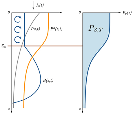
Figure 1. Sketch of the basic model relations with respect to depth. With the information on surface irradiance I₀(t) and the optical properties of the water column, the irradiance at depth I(z, t) (gray curve) is first calculated. Using I(z, t) and the photosynthesis irradiance function p^B(I), along with the information on biomass B(z, t) (blue curve on the left hand side), normalized instantaneous production P^B(z, t) is obtained (orange curve). Further on, taking the product of B(z, t) and P^B(z, t) and integrating it over time we get the daily production at depth (blue curve on the right hand side). In this depiction watercolumn production P_{Z, T} is the blue surface under the P_T(z) curve. Blue arrows indicate mixing and Z_m marks the mixed layer depth. Daily production from the surface up to Z_m is marked with P_Zm,T.

Using dimensional analysis Platt and Sathyendranath (1993) showed that the canonical form for the solution of integral (2), in the case of vertically uniform biomass B(z, 0) = B, is:

$\begin{array}{rc}{P}_{Z,T}~\frac{B{P}_m^{B}D}{K}f(I_{*}^m),& (4)\end{array}$

where K is the diffuse attenuation coefficient for downward irradiance (Kirk, 2011) and $I_{*}^m={\alpha }^B{I}_0^m/P_m^B$ the scaled noon irradiance, with $I_0^m$ as noon irradiance. The $f(I_{*}^m)$ function is determined by the formulation of the production-light relationship. In case of the Platt photosynthesis irradiance function (Platt et al., 1980):

$\begin{array}{rc}{p}^B(I)=P_m^B\left(1-\exp \left(-{\alpha }^{B}I/P_m^B\right)\right),& (5)\end{array}$

the $f(I_{*}^m)$ is:

$\begin{array}{l}f(I_{*}^m)={\displaystyle \sum _{n=1}^{\infty }\frac{2{\left(I_{\ast }^m\right)}^{2n-1}}{\pi \left(2n-1\right)\left(2n-1\right)!}}\frac{\left(2n-2\right)!!}{\left(2n-1\right)!!}\\ -{\displaystyle \sum _{n=1}^{\infty }\frac{{\left(I_{\ast }^m\right)}^{2n}}{2n\left(2n\right)!}}\frac{\left(2n-1\right)!!}{\left(2n\right)!!}.& (6)\end{array}$

In that case the exact solution to integral (2) is:

$\begin{array}{rc}{P}_{Z,T}=\frac{B{P}_m^{B}D}{K}f(I_{*}^m).& (7)\end{array}$

When the water column is of a finite depth Z_m (Figure 1) the solution is:

$\begin{array}{rc}{P}_{Z_m,T}=\frac{B{P}_m^{B}D}{K}\left(f(I_{*}^m)-f(I_{*}^m{e}^{-K{Z}_m})\right).& (8)\end{array}$

This solution was derived by Platt et al. (1990) and thus far no other analytical solution for watercolumn production has been reported in the literature. It is called the canonical solution. The assumptions of the model regarding light conditions are: optically-uniform water column with sinusoidally varying surface irradiance, such that the irradiance at depth is given by:

$\begin{array}{rc}I(z,t)=I_0^m\sin (\pi t/D)e^{-Kz}.& (9)\end{array}$

Inserting this expressions into (5) gives the biomass normalized production as:

$\begin{array}{rc}{P}^B(z,t)=P_m^B\left(1-\exp \left(-{\alpha }^B{I}_0^m\sin \left(\pi t/D\right)e^{-Kz}/P_m^B\right)\right).& (10)\end{array}$

Time integral of P^B(z, t) gives the daily normalized production $P_T^B(z)$. Here we shall use this same model setup but will relax the assumptions of homogeneous and constant biomass. We will allow for time- and depth-dependent biomass, seek the solution for P_Z,T in specific situations and explore the influence that a time-, or depth-, dependent biomass has on watercolumn production. Therefore, in this paper, a more complete definition for P_Z,T would be:

$\begin{array}{rc}{P}_{Z,T}={\displaystyle \underset{0}{\overset{D}{\int }}{\displaystyle \underset{0}{\overset{\infty }{\int }}B}}(z,t)P^B(z,t)\text{\hspace{0.17em}d}z\text{\hspace{0.17em}d}t.& (11)\end{array}$

A complete list of symbols with corresponding descriptions is given in Appendix A.

Biomass Specification

As formulated, this watercolumn production integral requires the specification of biomass as a function of depth and time. To specify biomass for integral (11) it is useful to write a differential equation for the time evolution of the biomass. In this way biomass dynamics are incorporated into the integral and its solution. The dynamics of biomass can be modeled by a simple equation of the following form:

$\begin{array}{rc}\frac{\partial }{\partial t}B(z,t)=\frac{1}{\chi }{P}^B(z,t)B(z,t),& (12)\end{array}$

Sathyendranath and Platt (2007) assuming the carbon to chlorophyll ratio χ constant during time (Sathyendranath et al., 2009). This equation governs the time evolution of biomass resulting from photosynthesis and allows for the accumulation of biomass at each depth in accordance with (10).

Let B*(z, t) be the solution to the growth equation (12). A direct approach for calculating P_{Z, T} would be to insert B*(z, t) into the integral (11) and solve for P_{Z, T}:

$\begin{array}{rc}{P}_{Z,T}={\displaystyle \underset{0}{\overset{D}{\int }}{\displaystyle \underset{0}{\overset{\infty }{\int }}{B}^{*}}}(z,t)P^B(z,t)\text{\hspace{0.17em}d}z\text{\hspace{0.17em}d}t.& (13)\end{array}$

With the usage of the solution B*(z, t) in (11), watercolumn production is coupled to the biomass dynamics expressed by (12). However, this approach can be mathematically complex, depending on the form of the solution B*(z, t). A simpler approach follows by recognizing that the process of biomass accumulation described by (12) is in fact primary production. Therefore, the difference between the final B*(z, D) and initial biomass B*(z, 0), multiplied by χ, equals daily primary production at depth z. Mathematically, the solution B*(z, t) satisfies (12) and the following holds:

$\begin{array}{rc}{B}^{*}(z,t)=\frac{\chi }{P^B(z,t)}\frac{\partial }{\partial t}{B}^{*}(z,t).& (14)\end{array}$

Inserting this expression into (13) and solving yields:

$\begin{array}{rc}{P}_{Z,T}=\chi {\displaystyle \underset{0}{\overset{\infty }{\int }}(}{B}^{*}(z,D)-B(z,0))\text{\hspace{0.17em}d}z.& (15)\end{array}$

This expression gives the watercolumn production as the difference between the final and initial biomass multiplied by the carbon to chlorophyll ratio. The two integrals, (13) and (15), are equivalent. The advantage of the second approach (15) is evident in cases when the biomass dynamics are governed by the simple growth equation, such as (12), whereas the first approach (13) is more useful when the solution to equation (12) is a simple mathematical expression. Both approaches will be used later.

If in the time interval from t = 0 (sunrise) until t = D (sunset) the following expression holds for the solution B*(z, t):

$\begin{array}{rc}\frac{\partial B^{*}(z,t)}{\partial t}\approx 0,& (16)\end{array}$

it is safe to assume B*(z, D) ≈ B*(z, 0) and justified to use initial biomass throughout the calculation of daily production. Biomass profiles of this type can be considered to be in, or close to, a steady state (Hodges and Rudnick, 2004). From the dynamical perspective this approach is crude, but solutions with initial biomass are valid in situations when the biomass does not change significantly during the time course of 1 day. In this sense, integral (2) is a special case of integral (13) when (16) is valid. The accumulation of biomass due to photosynthesis is either not significant compared with the initial biomass, or is balanced by the loss processes. With this approach, the functional form of the initial biomass profile can be inferred from measurement, instead of by solving the model equations, which is an advantage. In fact, this is the standard practice in remote sensing applications (Platt and Sathyendranath, 1988; Behrenfeld and Falkowski, 1997).

Stratified, Time-Independent Biomass

In summer periods of intense heating and weak mixing, strong stratification in temperature, as well as stratification in biomass, tend to develop below the mixed layer (Mann and Lazier, 2006). In this stratified region, the biomass tends to remain virtually constant in time, with only slight fluctuations in the shape of the chlorophyll profile as the season advances. In the tropical ocean stratification can be a permanent feature, whereas in the temperate regions stratification tends to be eroded during autumn and winter (Longhurst and Harrison, 1989). Given that stratification usually persists for intervals of time longer than 1 day, it is safe to assume constant biomass when calculating daily watercolumn production. Depth variation in biomass is assumed to have a larger influence on the magnitude of daily watercolumn production than time dependence does. Mathematically, integral (2) is appropriate in these conditions and model solutions with time-independent biomass are valid, because we assume that biomass does not change significantly during the time course of 1 day, as stated by (16). This assumption is valid in regions of the ocean where a stratified biomass profile is observed to be persistent on time scales longer than that of 1 day.

General Case

When the biomass profile is held constant in time B(z, 0) = B(z), a link between the canonical solution and the general solution to integral (2) can be established. To demonstrate this relation, we take advantage of the daily normalized production profile $P_T^B(z)$. With it, integral (2) becomes:

$\begin{array}{rc}{P}_{Z,T}={\displaystyle \underset{0}{\overset{\infty }{\int }}B}(z)P_T^B(z)\text{\hspace{0.17em}d}z.& (17)\end{array}$

In this way, watercolumn production is given as an integral of the product between the time-independent biomass B(z) and normalized daily production $P_T^B(z)$. The solution for the daily normalized production profile $P_T^B(z)$ in case of the Platt et al. (1980) photosynthesis irradiance function (5) is Kovač et al. (2016a):

$\begin{array}{rc}{P}_T^B(z)=P_m^{B}D{f}_z(I_{*}^m{e}^{-Kz}),& (18)\end{array}$

where the $f_z(I_{*}^m{e}^{-Kz})$ function is related to the $f(I_{*}^m)$ function in the following manner:

$\begin{array}{rc}{f}_z(I_{*}^m{e}^{-Kz})=-\frac{1}{K}\frac{\text{d}}{\text{d}z}f(I_{*}^m\exp (-Kz)).& (19)\end{array}$

Inserting this expression into (17) and solving by partial integration gives:

$\begin{array}{rc}{P}_{Z,T}=\frac{P_m^{B}D}{K}(B(0)f\left(I_{*}^m\right)+{\displaystyle \underset{0}{\overset{\infty }{\int }}\frac{\text{d}B\left(z\right)}{\text{d}z}}f\left(I_{*}^m{e}^{-Kz}\right)\text{d}z),& (20)\end{array}$

Where we have used $B(\infty )f(I_{*}^m{e}^{-K\infty })=0$. The first term on the right hand side is simply the canonical solution (7) and the second term is recognized as the contribution arising from the shape of the biomass profile (stratification term).

The interpretation of the first term is simple: it gives the watercolumn production in the case where surface biomass stretches over the entire watercolumn. According to the second term, any change in biomass with depth causes a deviation from the canonical solution. If there is an increase in biomass, dB(z)/dz > 0, this contribution is positive, whereas if there is a decline, dB(z)/dz < 0, this contribution is negative. The change in biomass dB(z)/dz is scaled by the $f(I_{*}^m{e}^{-Kz})$ function. The product $dB(z)f(I_{*}^m{e}^{-Kz})$ equals the production that would occur below the depth z in case the biomass from z to ∞ were equal to dB(z). Total contribution from all these infinitesimal changes in B(z) is accounted for by the integral on the right hand side of (20). With increase in depth, the contribution from biomass variation decreases, simply because production declines with increasing depth (10).

Expression (20) is a formal relation linking the canonical solution (7) to the solution for watercolumn production with stratified biomass (2). It is valid for an arbitrary biomass profile and clearly displays the role surface biomass B(0) has on the magnitude of P_{Z, T}. Surface biomass appears as a leading factor in P_{Z, T}. The significance of this result is emphasized given that surface biomass is readily accessible to satellite measurement. Therefore, if the remotely-sensed surface biomass is precise, and assuming the remaining parameters of the model are characteristic of the ocean region in question, the error in the estimated watercolumn production arises solely as a consequence of the error in estimating the biomass profile, which is inaccessible to remote sensing and has to be assigned based on prior information (Platt and Sathyendranath, 1988).

Shifted Gaussian Biomass Profile

An important case of the time independent biomass profile is that of the shifted Gaussian superimposed on a constant background. The shifted Gaussian is a suitable function for the description of the vertical structure of biomass for diverse regions of the oceans (Platt et al., 1991b), especially for the case of the widespread deep chlorophyll maximum (Longhurst, 1998; Mignot et al., 2014). In remote sensing applications it has been widely used to model biomass profiles in algorithms for primary production calculation (Platt and Sathyendranath, 1988, 1991). It is also used in operational oceanography (Platt et al., 2008), with well-established and tested procedures (Platt et al., 1988; Longhurst et al., 1995). The role of the shifted Gaussian in ocean color remote sensing has been studied and modeled by many authors, including: Morel and Berthon (1989), Sathyendranath and Platt (1989), Andre (1992), Stramska and Stramski (2005), Uitz et al. (2006), Xiu et al. (2008), and Mignot et al. (2011).

In this case the biomass profile equals:

$\begin{array}{rc}B(z)=B_0+\frac{h}{\sigma \sqrt{2\pi }}\exp \left(-\frac{{(z-z_m)}^2}{2{\sigma }^2}\right),& (21)\end{array}$

where the integrated biomass beneath the Gaussian curve is given by h, the depth of the maximum is at z_m and the width of the biomass peak is determined by σ. B₀ is the background biomass. The peak biomass above the background B₀ at z_m is $H=h/(\sigma \sqrt{2\pi })$. Upon inserting this expression into integral (17) we get:

$\begin{array}{rc}{P}_{Z,T}={\displaystyle \underset{0}{\overset{\infty }{\int }}{B}_0}{P}_T^B(z)dz+{\displaystyle \underset{0}{\overset{\infty }{\int }}\frac{h}{\sigma \sqrt{2\pi }}}\exp \left(-\frac{{(z-z_m)}^2}{2{\sigma }^2}\right)P_T^B(z)\text{d}z.& (22)\end{array}$

The first integral can be replaced with the canonical solution and the second integral can be simplified with the help of (18) to give:

$\begin{array}{l}{P}_{Z,T}=\frac{B_0{P}_m^{B}D}{K}f(I_{*}^m)\\ +\frac{h{P}_m^{B}D}{\sigma \sqrt{2\pi }}{\displaystyle \underset{0}{\overset{\infty }{\int }}\exp }\left(-\frac{{(z-z_m)}^2}{2{\sigma }^2}\right)f_z\left(I_{*}^m{e}^{-Kz}\right)\text{d}z.& (23)\end{array}$

With reference to (20) we label the second term on the right hand side as ΔP_{Z, T} (stratification term). The exact mathematical derivation of the solution for ΔP_{Z, T} is given in the Appendix B. The final solution is:

$\begin{array}{l}\Delta P_{Z,T}=P_m^{B}D\frac{h}{2}[{\displaystyle \sum _{n=1}^{\infty }\exp }\left(\frac{z_{2n-1}^2-z_m^2}{2{\sigma }^2}\right)\frac{2{\left(I_{*}^m\right)}^{2n-1}}{\pi \left(2n-1\right)!}\frac{\left(2n-2\right)!!}{\left(2n-1\right)!!}\left(1+\Phi \left(\frac{z_{2n-1}}{\sqrt{2}\sigma }\right)\right)\\ -{\displaystyle \sum _{n=1}^{\infty }\exp }\left(\frac{z_{2n}^2-z_m^2}{2{\sigma }^2}\right)\frac{{\left(I_{*}^m\right)}^{2n}}{\left(2n\right)!}\frac{\left(2n-1\right)!!}{\left(2n\right)!!}\left(1+\Phi \left(\frac{z_{2n}}{\sqrt{2}\sigma }\right)\right)],& (24)\end{array}$

where Φ is the error function, $z_{2n-1}=z_m-(2n-1){\sigma }^{2}K$ and $z_{2n}=z_m-2n{\sigma }^{2}K$. The complete solution to (22) is now:

$\begin{array}{rc}{P}_{Z,T}=\frac{B_0{P}_m^{B}D}{K}f(I_{*}^m)+\Delta P_{Z,T},& (25)\end{array}$

where the ΔP_{Z, T} depends explicitly on the values of h, z_m, σ, α^B, $P_m^B$, $I_0^m$, and D. This expression calculates the amount of carbon assimilated during 1 day per meter squared of the ocean surface, by phytoplankton distributed vertically according to the shifted Gaussian function (21).

The shifted Gaussian is flexible enough to describe various features in the measured chlorophyll profiles and therefore this solution covers a wide range of situations encountered in the field. That flexibility is achieved by altering the parameters of the function, namely: B₀, z_m, σ, and h. The disadvantage is that in addition to the six basic quantities: α^B, $P_m^B$, B₀, $I_0^m$, D, and K, which appear in the canonical solution, the solution for the shifted Gaussian has three more: z_m, σ, and h. To apply the solution, the values of these quantities need to be specified.

Time-Dependent, Mixed-Layer Biomass

Accounting for time dependence may be advantageous when considering mixed-layer production, especially during the period of a bloom. Blooms are typically initiated by stratification, either from heating, river discharge or from sea ice melt (Mann and Lazier, 2006). After the onset of stratification, the phytoplankton become trapped in the upper, well-illuminated, nutrient-rich layer, where conditions for growth are fulfilled, and in this upper layer production is most intense, which can lead to rapid accumulation of biomass (Chiswell et al., 2015). Blooms last until nutrients are depleted, after which they crash (Levy, 2015), or are terminated by overgrazing. How rapidly the bloom develops will be determined by physical conditions, the physiological status of the phytoplankton population and by loses (Banse and English, 1994), resulting in diverse patterns of seasonal cycles of phytoplankton biomass, as evident in remotely sensed records of chlorophyll concentration (Vargas et al., 2009; Racault et al., 2012). In the model, the physiological status is described by the photosynthesis irradiance function, whereas the physical conditions are presented by the mixed layer depth, surface irradiance, and the attenuation coefficient. Next, we calculate primary production in the mixed layer and show how it is affected by rapidly-growing or declining biomass.

Increasing Mixed-Layer Biomass

Let us consider a mixed layer of depth Z_m (constant in time) with uniformly-distributed biomass at initial time B(z, 0) = B₀, for z = 0 to z = Z_m. To simplify the equations, we introduce the following notation for the total biomass in the mixed layer:

$\begin{array}{rc}{B}_{Z_m}(t)={\displaystyle \underset{0}{\overset{Z_m}{\int }}B}(z,t)\text{\hspace{0.17em}d}z.& (26)\end{array}$

At time t = 0 the total biomass is B_Zm(0) = B₀Z_m. Let us also assume that the newly-synthesized mixed layer biomass at time t is redistributed through the mixed layer during a time interval Δt, so that there is no stratification in biomass at t + Δt. Mixed-layer biomass at time t + ΔT is now:

$\begin{array}{rc}{B}_{Z_m}(t+\Delta t)=B_{Z_m}(t)+\frac{1}{\chi }{P}_{Z_m}(t)\Delta t,& (27)\end{array}$

with P_Zm(t) given as $P_{Z_m}(t)=\underset{0}{\overset{Z_m}{\int }}P(z,t)dz$. In the limit of Δt → 0, that is instantaneous mixing of newly-synthesized biomass, this equation reduces to:

$\begin{array}{rc}\frac{\partial }{\partial t}{B}_{Z_m}(t)=\frac{1}{\chi Z_m}{P}_{Z_m}^B(t)B_{Z_m}(t).& (28)\end{array}$

Derivation of this equation is given in the Appendix C. The solution for the mixed-layer production with time-dependent biomass described by (28) and initial biomass B_Zm(0) = B₀Z_m is:

$\begin{array}{rc}{P}_{Z_m,T}=\chi B_0{Z}_m\left[\exp \left[\frac{P_m^{B}D}{\chi Z_{m}K}(f(I_{*}^m)-f(I_{*}^m{e}^{-K{Z}_m}))\right]-1\right].& (29)\end{array}$

The solution is found by the application of (15); details are given in the Appendix C. The term in the exponent is recognized as the canonical solution (8) divided by χ, Z_m, and B₀. It is clear that the canonical solution (8) will underestimate production in comparison with this solution. Due to photosynthesis, at a given moment there will be more biomass in the mixed layer, than in the case of time-independent biomass.

Declining Mixed-Layer Biomass

Given that the term P^B(z, t) is always positive, we have considered so far only the case of growing biomass. Here we consider the case when this term is reduced in magnitude by a loss term, and investigate the effect biomass loss has on the magnitude of daily production. With this goal, equation (12) is modified by addition of a loss term in the most general form L^B:

$\begin{array}{rc}\frac{\partial }{\partial t}B(z,t)=\left(\frac{1}{\chi }{P}^B(z,t)-L^B\right)B(z,t).& (30)\end{array}$

For there to be a negative growth (decline) in biomass the term L^B has to be greater than P^B(z, t):

$\begin{array}{rc}{L}^B\gg \frac{1}{\chi }{P}^B(z,t).& (31)\end{array}$

In this case the solution to equation (30) at time t is:

$\begin{array}{rc}B(z,t)=B_0{e}^{-L^{B}t},& (32)\end{array}$

where we have used the initial condition B(z, 0) = B₀. Time dependence of this type is often observed in satellite records of surface biomass, for example during the termination phase of a bloom (Cabre et al., 2016). Therefore, to calculate mixed layer production in this case, we insert the previous expression into (11) and obtain the following integral:

$\begin{array}{rc}{P}_{Z_m,T}={\displaystyle \underset{0}{\overset{D}{\int }}{\displaystyle \underset{0}{\overset{Z_m}{\int }}{B}_0}}{e}^{-L^{B}t}{P}^B(z,t)\text{\hspace{0.17em}d}z\text{\hspace{0.17em}d}t.& (33)\end{array}$

This procedure is in accord with (13). The derivation of the solution to this integral is given in the Appendix D. The final solution is:

$\begin{array}{l}{P}_{Z_m,T}=\frac{B_0{P}_m^{B}D}{K}[(e^{-L^{B}D}+1){\displaystyle \sum _{n=1}^{\infty }\frac{{\left(I_{*}^m\right)}^{2n-1}-{\left(I_{*}^m{e}^{-K{Z}_m}\right)}^{2n-1}}{\pi (2n-1)}}{\displaystyle \prod _{m=1}^n\frac{1}{{(-L^{B}D/\pi )}^2+{(2m-1)}^2}}\\ -\frac{(e^{-L^{B}D}-1)}{-L^{B}D}{\displaystyle \sum _{n=1}^{\infty }\frac{{\left(I_{*}^m\right)}^{2n}-{\left(I_{*}^m{e}^{-K{Z}_m}\right)}^{2n}}{2n}}{\displaystyle \prod _{m=1}^n\frac{1}{{(-L^{B}D/\pi )}^2+{(2m)}^2}}].& (34)\end{array}$

In the expression inside the square brackets, the loss term L^B and daylength D appear as a product L^BD, which imposes itself as a dimensionless factor for the problem, determining just how much the continual loss of initial biomass reduces watercolumn production. This type of loss can occur when the grazing pressure on phytoplankton is significant, or by sinking out of the mixed layer. Potentially, the magnitude of the loss term could be determined from time series of satellite-estimated surface chlorophyll.

Relation to the Canonical Solution

In case of increasing, mixed layer biomass, the canonical solution (8) is easily recognized in the exponential function on the right hand side of expression (29). Writing the exponential as a sum and rearranging, gives:

$\begin{array}{l}{P}_{Z_m,T}=\frac{B_0{P}_m^{B}D}{K}\left(f\right(I_{*}^m)-f(I_{*}^m{e}^{-K{Z}_m}))\\ +B_0{\displaystyle \sum _{n=2}^{\infty }\frac{{(P_m^{B}D)}^n}{n!{(\chi Z_m)}^{n-1}{K}^n}}{(f(I_{*}^m)-f(I_{*}^m{e}^{-K{Z}_m}))}^n.& (35)\end{array}$

The first term on the right hand side is the canonical solution (8) and the additional terms arise due to time dependent biomass. When the biomass is time independent, as is the case with the canonical solution, these terms will vanish. Therefore, when biomass is time dependent the canonical solution (8) can be interpreted as the first order approximation for mixed layer production, representing the lower limit on watercolumn production. Important to note is that biomass has to increase with time in accordance with (28) for this interpretation to hold.

On the other hand, when biomass is declining with time, as stated in (32), the canonical solution will be the upper limit on daily watercolumn production, given that at each time instant there is less biomass in the mixed layer, in comparison with constant biomass B₀. In this case we were unable to find an exact link between solution (34) and the canonical solution. Instead, we have found by numerical exercises, the canonical solution with noon biomass $B_0{e}^{-L^{B}D/2}$, in place of initial biomass B₀, to be a good approximation for the full solution (34):

$\begin{array}{rc}{P}_{Z_m,T}\approx B_0{e}^{-L^{B}D/2}\frac{P_m^{B}D}{K}(f(I_{*}^m)-f(I_{*}^m{e}^{-K{Z}_m})).& (36)\end{array}$

It is important to emphasize the initial assumption behind solution (34). For it to hold, the loss rate has to be significantly larger than normalized production (31) so that the growth due to production is insignificant in comparison with losses and (32) is valid. Therefore, solution (34) is valid when (31) holds and the approximation (36) is only then justified.

3. Data

The models described so far and the solutions derived therefrom require parameter values to be implemented and tested against data. Oceanic time series are suitable sources of such information. For our model, the Hawaii Ocean Time-series (HOT) is an ideal testing ground. Data from it have already served for other model testing, with over 600 publications testifying to the quality of the data. The entire data set is publicly available with full documentation of the methods and procedures used. Information on the data set can be found in Karl et al. (2001) and Karl and Church (2014).

HOT is a program of oceanic measurements started in 1988 at station Aloha, located near the Hawaii Islands at 22°45′N 158°W. The basic set of measurements relevant for this model encompasses: primary production using the standard in-situ implemented ¹⁴C method (Steemann Nielsen, 1952), fluorimetric determination of chlorophyll concentration (Strickland and Parsons, 1972), optical measurements using bio-optical profilers, surface photosynthetically-available radiation (PAR) measurement using on deck radiometer, and finally the mixed-layer depth determination based on potential density.

There are in total 194 cruises with available data. Production and chlorophyll were measured at: 5, 25, 45, 75, 100, 125, 150, and 175 m. Surface PAR was given in μ E m⁻² s⁻¹ and the conversion to W m⁻² was done using Smith and Morel's procedure (Morel and Smith, 1974). From it $I_0^m$ was determined as ${\tilde{I}}_0^m={\tilde{I}}_T\pi /2D$, where ${\tilde{I}}_T$ is the total received irradiance throughout the day. Daylength was provided from PAR measurement. The diffuse attenuation coefficient was calculated from one percent light level which was given for 150 cruises, based on optical profiles. For the remaining cases, the average value of 0.0435 m⁻¹ has been used. Mixed-layer depth Z_m was estimated by the offset of 0.125 kg m⁻³ in potential density at depth, from the surface value (de Boyer Montegut et al., 2004; Suga et al., 2004). Photosynthesis parameters were estimated from chlorophyll and production profiles using the method of Kovač et al. (2016a,b). The data on production, chlorophyll, PAR, one percent light depth and mixed layer depth are publicly available at hahana.soest.hawaii.edu/hot, whereas the data on the photosynthesis parameters are publicly available at jadran.izor.hr/~kovac/parameters. There were no data on the carbon-chlorophyll ratio.

With the available data, we now proceed to test the solution for the mixed layer production and the shifted Gaussian solution. We further use the solutions with time dependent biomass to predict the influence that time-dependent biomass exerts on mixed layer production. For the measured/known value of a variable/parameter we use $\widetilde{,}$, e.g., $\tilde{x}$, whereas for a model variable/parameter we use ordinary symbols, e.g., x.

4. Results

Testing the Canonical Solution for Mixed-Layer Production

A straightforward way of testing the canonical solution is simply to calculate mixed layer production with it. The mixed layer is by definition a region of uniform biomass and the assumption of uniformity in biomass required by the canonical solution is fulfilled. To test the model structure we calculate mixed-layer production with expression (8) and compare it with the measured mixed layer production, calculated with the trapezoidal rule from the measured production profile. The obtained results are displayed in Figure 2.

FIGURE 2

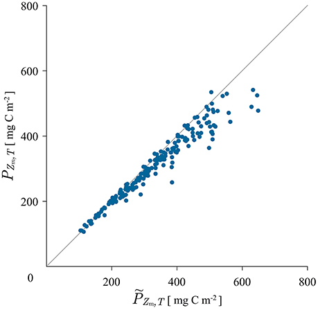
Figure 2. Scatter plot of measured mixed layer production ${\tilde{P}}_{Z_m,T}$ calculated with the trapezoidal rule from the measured production profile and modeled mixed layer production P_Zm,T calculated with the canonical solution (8) using the average measured biomass from 5 to 25 m depth.

For the mixed-layer biomass in expression (8) the average value of the measured biomass from the first two measuring depths was used. As can be seen from the figure, the match between the modeled and the measured mixed-layer production is quite satisfactory. The coefficient of determination is r² = 0.94. Therefore, the canonical solution is a good model for mixed-layer production. Some discrepancy is seen at higher values of production. These errors may be caused by the way in which the mixed-layer depth was estimated. It may not always be the case that the mixed layer depth estimated from potential density corresponds well with the depth of active mixing and it is the depth of active mixing that is relevant for biomass homogenization (Franks, 2015). In some data sets we have observed the biomass not to be homogeneous from the surface all the way down to the base of the mixed layer estimated from potential density. This increase in biomass causes more production, than would otherwise occur without it and is reflected in the slight deviation in Figure 2.

Testing the Shifted Gaussian Solution

A prerequisite in the application of the solution (25) is to know the values for the parameters of the shifted Gaussian. These have to be estimated from HOT data on chlorophyll profiles. To obtain the biomass parameters we have fitted the shifted Gaussian to the measured chlorophyll profiles by adjusting the parameter values. The conjugate gradient method was used (Baldick, 2006; Knyazev and Lashuk, 2008). The shifted Gaussian was convergent for each chlorophyll profile. Average concentration of background biomass B₀ is 0.085 mg Chl m⁻³, with a standard deviation of 0.025 mg Chl m⁻³. Average depth of the deep chlorophyll maximum z_m is 104.12 m, with a standard deviation of 19.00 m. Average width of the biomass peak σ is 21.93 m, with a standard deviation of 8.89 m, and finally the average height of the biomass peak H is 0.175 mg Chl m⁻³, with a standard deviation of 0.075 mg Chl m⁻³.

With the estimated parameters we have further calculated the accuracy of representing the measured biomass profiles with the shifted Gaussian. The biomass given by the shifted Gaussian was calculated at the depth of each measurement and compared with the measured value. The results are shown in Figure 3. There are in total 1552 measurements of chlorophyll. As can be seen, the shifted Gaussian is a good model for the biomass profile at all the measuring depths except the last two (150 and 175 m). The coefficient of determination for the data from all depths is 87.84%. However, once the last two depths are excluded the coefficient of determination jumps to a high 98.39%, signifying that the shifted Gaussian is an even better model for the biomass up to the measurement depth of 125 m. The contribution to watercolumn production from depths >125 m is expected to be minimal.

FIGURE 3

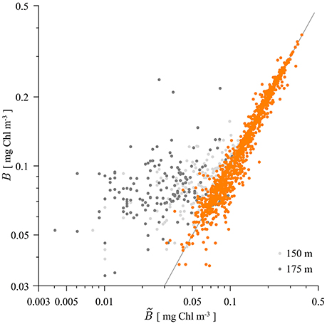
Figure 3. Scatter plot of measured $\tilde{B}$ and modeled biomass B with the shifted Gaussian (21). The first six measurement depths are given in orange, whereas the data from 150 m measurement depth is given in light gray and the data from 175 m measurement depth is given in gray. The gray line represents the 1:1 model vs. data ratio. For the points above/below the gray line the shifted Gaussian overestimates/underestimates the measured biomass.

The results of applying the analytical solution (24) are displayed in Figure 4. The solution did not exhibit convergent behavior for all the cruise data: out of 194, it converged for 168 cruises. The reason for divergence in the remaining 26 cruises comes from the behavior of the exponential terms $exp((z_{2n-1}^2-z_m^2)/2{\sigma }^2)$ and $exp((z_{2n}^2-z_m^2)/2{\sigma }^2)$, which upon summation in solution (24) divergee when σ is high and z_m is small. This corresponds to the case of a wide chlorophyll maximum close to the surface. The solution behaves well when σ is small and z_m large, which is the case of a narrow deep maximum, i.e., a deep chlorophyll maximum. As a measure of the applicability of the given solution the 3σ rule can be applied. For the Gaussian function 99% of the biomass concentration above B₀ is located in the depth interval (z_m−3σ, z_m + 3σ). When z_m is larger than 3σ this biomass is located below the surface. That is the dominant situation at HOT station and the solution converges, as evident in Figure 4.

FIGURE 4

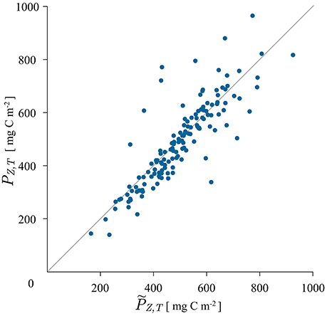
Figure 4. Scatter plot of measured watercolumn production ${\tilde{P}}_{Z,T}$, calculated with the trapezoidal rule from the measured production profile, and modeled watercolumn production P_{Z, T}, calculated with the analytical solution for the shifted Gaussian biomass (24). The solution did not converge for 26, out of 194 tested cruises.

Predictions with the Time-Dependent Biomass Solutions

Application of the canonical and the shifted Gaussian solutions is straightforward, given that all the necessary parameters are available. The solutions with time-dependent biomass are more complex to apply due to the requirement for additional parameter values. However, even without knowledge of these parameter magnitudes, the solution can be used to estimate the effect of growth, or decline, in biomass on the magnitude of mixed-layer production. If the biomass is allowed to accumulate, then production is expected to increase in comparison with the case for a time-independent biomass. The opposite holds for the case of a decline in biomass. Just how strong these effects are can easily be calculated for hypothetical cases, but to be as close as possible to real scenarios we apply the solutions with the parameter values typical of HOT.

To illustrate our point, we calculate mixed-layer production using the new solutions with the median values for the mixed-layer depth, assimilation number, mixed-layer biomass, and the attenuation coefficient from HOT. We plot the solutions as a function of the dimensionless noon irradiance to demonstrate the effect light has on the magnitude of mixed-layer production (Figure 5). In this exercise daylength D is set to 10 h. The blue curve on the figure gives the canonical solution for mixed layer production with the median parameter values: Z_m = 54.75 m, $P_m^B=7.85$ mg C (mg Chl)⁻¹ h⁻¹, B = 0.072 mg Chl m⁻³, and K = 0.043 m⁻¹. The orange curve is the solution (29) with the carbon-chlorophyll ratio equal to 150 mg C (mg Chl)⁻¹ and the light orange with the carbon-chlorophyll ratio equal to to 100 mg C (mg Chl)⁻¹. As expected, the production is higher when increase in biomass is accounted for. The red curve corresponds to the solution (34) with the dimensionless factor L^BD = 1. In this example D = 10 h, which gives L^B = 0.1 h⁻¹, i.e., a 10% decrease of biomass per hour. At this rate the biomass at sunset declines to its e-folding value B(D) = B₀/e. Finally the pink curve is the approximation (36), of the solution (34), with the same parameter values.

FIGURE 5

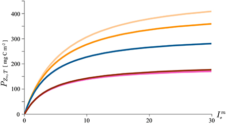
Figure 5. Mixed layer production calculated with the canonical solution (8, blue curve), solution for growing biomass (29, two orange curves with different carbon-chlorophyll ratio), the solution with declining biomass (34, red curve) and the approximation to the solution with declining biomass (36, pink curve). The parameters used in the solutions are typical of the Hawaii area and are given by the median values of: Z_m = 54.75 m, $P_m^B=7.85$ mg C (mg Chl)⁻¹ h⁻¹, B = 0.072 mg Chl m⁻³, and K = 0.043 m⁻¹. Daylength D is set to 10 h, the dimensionless factor L^BD to 1, carbon to chlorophyll ratio χ to 150 mg C (mg Chl)⁻¹ (orange curve) and to 100 mg C (mg Chl)⁻¹ (light orange curve).

In both cases the effect on mixed layer production is significant. The effect of growth is more pronounced for phytoplankton with lower values of carbon-chlorophyll ratio. This is simply understood by considering that for higher value of χ more carbon is required for a unit increase of chlorophyll. Mathematically, χ appears in the denominator in equation (28) signifying that the change in biomass per unit time is inversely proportional to χ. A straightforward conclusion is that the growth effect on primary production will be more pronounced for phytoplankton with lower values of χ and vice versa. The effect of loss on primary production is also straightforward: the decline of biomass during the day results in lower production. The greater the loss, the greater the diminution in production in comparison with the canonical solution. The exact magnitude of the reduction is now easily calculated using solution (34). The agreement between the approximation (36) with the exact solution (34) is remarkable.

5. Discussion

Taken together, the solutions presented cover a wide range of different mixing and growth conditions (Figure 6), such as might be encountered in the field: from intense mixing and low growth—canonical solution (8), intense mixing and high growth—increasing mixed-layer biomass solution (29), intense mixing and negative growth—declining mixed-layer biomass solution (34), and finally low mixing and low growth—shifted Gaussian solution (24). As all these conditions are indeed observable at times in the ocean, so too are the assumptions of the outlined solutions fulfilled to some extent, and the application of the solutions justified. The only case not solved here is of low mixing and high growth in biomass, which corresponds to the case of time-dependent stratified biomass. Analytical solution to this problem has yet to be found and is a potential topic for future theoretical work. The problem can be treated as formulated in this work, by first solving the growth equation for biomass (12) and inserting the solution directly into the integral for watercolumn production with time-dependent biomass (11).

FIGURE 6

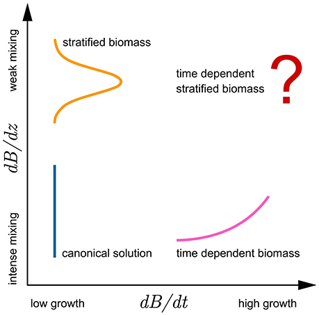
Figure 6. Conceptual diagram highlighting the relations of the model assumptions and analytical solutions with respect to growth (abscissa) and mixing (ordinate). Growth is presented as change in biomass over time dB/ dt, whereas the effects of mixing are presented as dB/ dz. Lines sketch the biomass profiles: orange for stratified biomass with week mixing and low growth, blue for uniform biomass with intense mixing and low growth, and pink for time dependent biomass with intense mixing. Solution for watercolumn production with time dependent stratified biomass has yet to be found.

Irrespective of the model, there are in essence three possible outcomes concerning temporal evolution of biomass. It can be constant, or accumulating or declining. Time dependence in biomass is easily seen in satellite records of chlorophyll (Racault et al., 2012; Cabre et al., 2016) which can potentially serve for assessing whether or not time dependence in biomass should be accounted for when calculating primary production. If the chlorophyll time series displays quiet periods with no temporal dependence in biomass, the canonical solution is then a valid model for mixed layer production. The model with increasing time-dependent biomass is adequate for primary production calculation during a blooming period. This period is also easy to diagnose from satellite chlorophyll time series. After the bloom crashes and the decline of chlorophyll begins to show in the record, the assumption behind the model with declining mixed-layer biomass becomes valid. The value of the loss rate can potentially be determined empirically from the chlorophyll record. Therefore, with respect to the annual cycle of biomass, the solutions presented in this work are each appropriate for a particular period of the year when their respective assumptions are met. Calculating annual watercolumn production in this manner can potentially be a topic for future research.

In earlier literature, integrals for watercolumn production were usually formulated with time-independent biomass (Platt and Sathyendranath, 1993) and could therefore be applied at any stage during the course of the annual cycle. Calculating production in this manner proved suitable for ocean areas where field biomass was known not to change considerably during the interval over which production was calculated, and was in a sense mandatory from the practical standpoint, given that observations of biomass were predominantly performed once per day. However, this approach resulted in biomass accumulation due to primary production having no effect on daily production. Formulating production integrals with biomass constant in time presumes incremental production due to newly-synthesized biomass as insignificant in comparison with production arising from initial biomass. The approach presented here alleviates this limitation and allows a positive feedback between biomass accumulation and primary production, with newly-synthesized biomass contributing to primary production.

The approach advocated here treats the temporal evolution of biomass as being governed by the growth equation, with the growth term dictated by instantaneous production. Coupling this equation to the watercolumn production integral was achieved through the reformulation of the integral via a time-dependent biomass term multiplying the normalized production term. Due to mathematical complexities of this formulation, different approaches for handling the problem were proposed. First, the problem of depth-dependent biomass was analyzed, with an important note that in this context it was viewed as a special case of a steady state solution for biomass distribution. Assuming steady state is reasonable for non-bloom conditions in the oligotrophic ocean, during summer periods at higher latitudes and below the mixed layer (Fennel and Boss, 2003). Biomass profiles of this sort are assumed to be solutions to a more complex equation for biomass, which accounts for other processes besides growth, such as losses by grazing, mixing, and sinking (Beckman and Hense, 2007). These processes are easily included in vertically resolved models for biomass, but the price paid for their inclusion is the increase in model complexity, which makes them difficult to solve analytically, with numerical procedures stepping in as the method of choice to obtain solutions (Huisman et al., 2002; Taylor and Ferrari, 2011).

To circumvent the problem of finding an analytical, steady-state solution to a more general equation, involving not only the nonlinear, time-dependent production term, but also sinking and mixing, we have employed the shifted Gaussian as an approximation to the solution for the biomass profile at steady state. The types of profiles described by the shifted Gaussian are indeed in close agreement with the numerical simulations of the biomass profiles (Beckman and Hense, 2007; Liccardo et al., 2013). More importantly, they are often obtained as results of measurements, and biomass profiles observed in the open ocean are a prototype example for using the shifted Gaussian in the integral for watercolumn production (Platt and Sathyendranath, 1988; Platt et al., 1991b). For vast regions of the open ocean biomass is vertically structured (Longhurst and Harrison, 1989). The most common structure is that of the deep chlorophyll maximum (Navaro and Ruiz, 2013), which is a perfect match for the shifted Gaussian. The deep chlorophyll maximum is often observed to be a quasi permanent feature, existing for months, if not for the duration of the whole annual cycle (Platt and Sathyendranath, 1988). In this case the processes that act to create the deep chlorophyll maximum, and sustain it, are in equilibrium on time scales longer than that of 1 day (Chiswell et al., 2015), justifying the assumption of time independent biomass in daily watercolumn production calculations. Deep chlorophyll maxima are also observed on majority of HOT cruises, with the shifted Gaussian demonstrated here to be a good model for HOT data (Figure 3). From this alone stems the legitimacy of using the shifted Gaussian as a model for the biomass profile in the watercolumn production integral for HOT.

In addition, when biomass remains stratified for prolonged periods of time it is safe to assume that mixing is not vigorous enough to distort the established stratification (Liccardo et al., 2013). Mixing itself is caused by various physical agents such as wind, waves, and convection (Franks, 2015), which increase turbulent kinetic energy in the mixed layer. In numerical models this process is parameterized with the mixing coefficient through turbulence closure schemes (Cushman-Roisin and Beckers, 2011). In the presented model however, mixing is not expressed explicitly, but rather the consequences of mixing are assumed implicit through the effect it had on shaping the initial biomass profile. In the field, uniform biomass profiles are most likely associated with strong mixing, whereas stratified biomass profiles are surely associated with less intense mixing. For if mixing were intense, stratification in biomass would not come about, because any incipient stratification would be quickly eroded. This process is well represented in numerical models of the biomass profile (Beckman and Hense, 2007). When assuming a uniform biomass profile we are in fact assuming that mixing was strong enough to cause homogenization of biomass.

This is of course valid for the mixed layer, in which biomass is homogeneous by definition, but it is important to make a distinction between the mixed layer and a layer of active mixing, as highlighted by Franks (2015). The solutions for mixed layer production presented here are strictly valid for a layer of active mixing, since we assume that mixing of newly-synthesized biomass is occurring instantaneously. However, it is often the case that mixed layer depth is determined based on density, or temperature, offset from the surface value (de Boyer Montegut et al., 2004), even though the mixed layer depth determined in this way may not always correspond well with the depth of active mixing (Franks, 2015). We suspect this to be the cause for the slight bias evident in Figure 2. For the model presented here, the assumption of active mixing is required to redistribute the newly-synthesized biomass so that growth occurs uniformly throughout the mixed layer.

Another relevant consequence of the assumption of active mixing is that it enabled the loss rate to be assumed vertically uniform in the mixed layer. In addition to vertical uniformity, not stating the loss rate explicitly left a certain flexibility in the presented model. The loss rate of the phytoplankton population is known to be a complex mixture of various processes such as mixing, sinking, predation, and mortality (Platt et al., 1991a; Zhai et al., 2010), and in the ocean these processes can combine to give a more complex pattern than simply a vertically-uniform loss rate. However, since the work of Sverdrup (1953), it is commonly assumed in theoretical considerations of mixed layer production that losses are in fact uniform due to mixing itself, and here presented model follows this basic approach.

Contrary to the loss rate, a basic feature of the model, shared also by all the previous models of watercolumn production (Platt and Sathyendranath, 1993), is depth resolved instantaneous production, caused by the decline of light intensity with depth. This allows for the accumulation of biomass in the growth equation to proceed in accord with the well established response of primary production to light, stated in (10). Therefore, production is given a more realistic treatment, than losses are. The lack of detailed treatment of the loss terms is not a serious drawback for this model, because parameterizations for respiration, excretion, grazing by micro- and macro-zooplankton, and sedimentation were already studied by Platt et al. (1991a) and Zhai et al. (2010). Inclusion of parametrization for losses given in Zhai et al. (2010) is straightforward here. Losses became as important as production in considerations of bloom dynamics and the model used here can shed some light on this topic, specifically on the Critical Depth Hypothesis.

Implications for the Critical Depth Hypothesis

The new formulation of the mixed-layer production model also has consequences for the Critical Depth Hypothesis. To demonstrate, let us again return to the case of the mixed layer with uniform biomass and the mixing depth given by Z_m. According to Sverdrup (1953), if the mixing depth is shallower than the critical depth Z_cr conditions for the initiation of a bloom are fulfilled (Siegel et al., 2002; Fischer et al., 2014). Critical depth is defined as the depth at which the mixed-layer production is balanced by mixed layer losses (Platt et al., 1991a; Sathyendranath et al., 2015) and is derivable from a conservation of biomass equation (Levy, 2015; Mignot et al., 2016). Mathematical formulations of the critical depth criterion are well established in the literature (Sverdrup, 1953; Platt et al., 1991a) and Sverdrup's criterion is usually acknowledged to be a necessary and a sufficient condition for bloom initiation, but not a sufficient condition for determining the amplitude of the bloom (Platt et al., 1994). It specifies whether the bloom can occur, but leaves the bloom amplitude unspecified. With the dynamic approach for primary production calculation, we now demonstrate that Sverdrup's criterion can also be used to calculate the daily increase in mixed layer biomass.

To elaborate, let us augment the production equation (28) with the loss term, so that the time evolution of mixed layer biomass becomes:

$\begin{array}{rc}\frac{\partial }{\partial t}{B}_{Z_m}(t)=\frac{1}{\chi Z_m}(P_{Z_m}^B(t)-L_{Z_m}^B)B_{Z_m}(t),& (37)\end{array}$

where $L_{Z_m}^B$ represents total losses in the broadest sense, arising from respiration, excretion, grazing, sinking, and so on (Zhai et al., 2010). Let the growth and loss of the mixed layer biomass be on the same order of magnitude. We assume the loss rate to be vertically uniform and time independent, a justifiable assumption given the mixing. The solution to this equation at time D + N, where N marks the night interval, is then:

$\begin{array}{rc}{B}_{Z_m}(D+N)=B_{Z_m}(0)\exp \left(\frac{1}{\chi Z_m}(P_{Z_m,T}^B-L_{Z_m,T}^B)\right).& (38)\end{array}$

If there is to be an increase in biomass during a 24 h period, that is:

$\begin{array}{rc}{B}_{Z_m}(D+N)>B_{Z_m}(0),& (39)\end{array}$

the term in the exponential function has to be greater than zero. It will be greater than zero when the mixed layer production surpasses the losses, that is $P_{Z_m,T}^B>L_{Z_m,T}^B$. Since the net production decreases with depth, because light intensity decreases and losses remain constant, there will be a depth at which the vertically-integrated production $P_{Z_m,T}^B$ equals vertically-integrated losses $L_{Z_m}^B$. The depth at which the two terms exactly balance $P_{Z_{cr},T}^B=L_{Z_{cr},T}^B$ is recognized as the critical depth Z_cr, defined by Sverdrup (1953). If the mixing depth is shalower than the critical depth the term in the exponential function is positive.

Invoking the canonical solution for $P_{Z_{cr},T}^B$ we get the implicit expression for the critical depth:

$\begin{array}{rc}\frac{P_m^{B}D}{K}(f(I_{*}^m)-f(I_{*}^m{e}^{-K{Z}_{cr}}))=L^B(D+N)Z_{cr},& (40)\end{array}$

where we have used $L_{Z_{cr,T}}^B=L^B(D+N)Z_{cr}$. Dividing both sides by Z_cr gives:

$\begin{array}{rc}\frac{P_m^{B}D}{K{Z}_{cr}}(f(I_{*}^m)-f(I_{*}^m{e}^{-K{Z}_{cr}}))=L^B(D+N).& (41)\end{array}$

This expression states that the average production in the mixed layer equals the average loss when the mixed layer depth is equal to the critical depth, which is precisely the critical depth criterion of Sverdrup (1953). Therefore, when the mixed layer extends to the critical depth there is no accumulation of biomass. Mixing beyond the critical depth leads to losses in the mixed-layer biomass, and finally mixing not extending to the critical depth leads to accumulation of mixed-layer biomass. The mathematical condition expressing this latter statement is simply:

$\begin{array}{rc}{Z}_m<Z_{cr},& (42)\end{array}$

with Z_cr given as a solution of (41). If this condition is met so is condition (39) and accumulation of mixed-layer biomass occurs. Whenever condition (42) is met, there will be a positive increase in mixed layer biomass over the course of 1 day of the following magnitude:

$\begin{array}{rc}\Delta B_{Z_m}=B_{Z_m}(0)\left[\exp \left(\frac{1}{\chi Z_m}(P_{Z_m,T}^B-L_{Z_m,T}^B)\right)-1\right].& (43)\end{array}$

The critical-depth criterion can now be restated as: when the mixed layer depth is shallower/deeper than the critical depth, there is an increase/decrease in mixed layer biomass of magnitude ΔB_Zm. If the critical depth and the mixed-layer depth are equal, the biomass remains constant.

Implications for Remote Sensing

Applying the models presented in this work as estimators of watercolumn production, based on remotely-sensed data on ocean color, is straightforward. The solutions can be used as a part of existing remote sensing algorithms for watercolumn production, requiring only alterations to be made on the module that calculates watercolumn production, with the analytical solutions taking place of the commonly employed numerical ones. The models are formulated in a similar fashion to our previous ones and when implemented require information on the same parameters and variables (Platt and Sathyendranath, 1993), of which the following are accessible by remote sensing: chlorophyll concentration, surface irradiance and the attenuation coefficient. A relevant distinction from the previous models concerns the assumption of time dependence in biomass. This has implications for remote sensing applications, given that all prior models assumed biomass constant in time, implying that sampling biomass at any time of the day was sufficient for these estimators. However, in the newly presented models temporal evolution of biomass is accounted for and we can ask how the biomass sampled at a specific time of day relates to the initial biomass required by the models.

Acknowledging that ocean color satellites have access to surface chlorophyll (approximately up to the first photic depth 1/K) and in line with the models presented so far, we write the equation for the time evolution of surface chlorophyll B(0, t) as:

$\begin{array}{rc}\frac{\partial }{\partial t}B(0,t)=\left(\frac{1}{\chi }{P}^B(0,t)-L^B\right)B(0,t),& (44)\end{array}$

ignoring advection and mixing, which makes it valid for laterally uniform fields, or for time scales short enough so that neither advection, nor mixing, cause significant changes in biomass over the course of integration. Let us assume that the satellite samples surface biomass at time t_s and label it $\tilde{B}(0,t_s)$. From the previous equation surface biomass at time t_s is:

$\begin{array}{rc}{B}^{*}(0,t_s)=B(0,0)\exp \left({\displaystyle \underset{0}{\overset{t_s}{\int }}}\left(\frac{1}{\chi }{P}^B(0,t)-L^B\right)\text{\hspace{0.17em}d}t\right).& (45)\end{array}$

Equating the remotely sensed biomass $\tilde{B}(0,t_s)$ with $B^{*}(0,t_s)$ enables as to express the initial surface biomass as:

$\begin{array}{rc}B(0,0)=\tilde{B}(0,t_s)\exp \left(-{\displaystyle \underset{0}{\overset{t_s}{\int }}\left(\frac{1}{\chi }{P}^B(0,t)-L^B\right)}\text{\hspace{0.17em}d}t\right).& (46)\end{array}$

This expression takes the remotely sensed biomass $\tilde{B}(0,t_s)$ and transforms it into the initial biomass B(0, 0), under the assumption that biomass evolves according to equation (44). It corrects the remotely sensed surface biomass for dynamical processes of growth and loss, to yield the initial biomass. Taking the satellite overpass time to be at local noon t_s = D/2, further enables us to express initial biomass explicitly as:

$\begin{array}{rc}B(0,0)=\tilde{B}(0,D/2)\exp \left(-\frac{D}{2}\left(\frac{P_m^B}{\chi }{f}_z(I_{*}^m)-L^B\right)\right).& (47)\end{array}$

According to these expressions, having dynamically evolving biomass in the model, affects not only the magnitude of watercolumn production, but also the way in which initial biomass should be calculated from remotely sensed biomass, to compensate for growth and loss. It is important to note that the correction is not linear, but exponential, with respect to production and loss.

6. Conclusions

The work presented here extends on the standard formulation of daily watercolumn production by allowing for depth- and time-resolved biomass. In the standard formulation, biomass was specified in advance and treated as unrelated to primary production (Platt and Sathyendranath, 1993), leaving prior models without proper dynamics in this regard. To avoid having this problem, we proposed an alternative approach and stated a growth equation for biomass, thus allowing for a time-dependent solution in biomass. Coupling this equation to the watercolumn production integral was achieved by reformulating the integral with time-dependent biomass. Therefore, biomass was related to growth, and as such, subsequently used in the watercolumn production integral.

Depth-resolved biomass was set via an initial condition and we distinguished two possibilities regarding depth dependence in biomass: stratified water column and a mixed layer. For the mixed layer, we further distinguished between growing and declining biomass, providing analytical solutions for watercolumn production in both cases. For the stratified water column we used the shifted Gaussian function to represent biomass profiles and derived an exact analytical solution for daily watercolumn production in this case. No analytical solutions to these problems have been reported in the literature until now.

The new solutions were tested with data from the HOT program. The shifted Gaussian was used to model biomass profiles and it was demonstrated to be a good model. The canonical solution for mixed layer production and the solution with the shifted Gaussian were applied as models of watercolumn production. Both analytical solutions proved to be good models for this open ocean station. The solutions for growing and declining biomass were used to predict mixed layer production in the cases where biomass was increasing/decreasing in accordance with the assumptions of the models.

Sverdrup's critical depth criterion was explored further and an exact expression for mixed layer biomass increment during 1 day was derived. The final statement of the critical depth criterion remained unaltered, although it was based on the argument of growth, whereas prior statements of the criterion were based on the balance between watercolumn production and losses (Sverdrup, 1953; Platt et al., 1991a). The two approaches are now seen equivalent with respect to the final outcome, that being the critical depth criterion.

It was further discussed how to merge the temporally-evolving surface biomass with the remotely-sensed surface biomass, to get to the initial condition on biomass. We expect the processes of growth and loss to affect surface biomass significantly during the initiation or termination phases of a bloom, when the biomass is changing rapidly on time scales shorter than 1 day. A potential course for future research would be to implement this approach in producing maps of chlorophyll from remotely-sensed data.

Author Contributions

CG and TP had the original ideas. TP, SS, and ŽK formulated the mathematical models. ŽK, TP, and SA solved the problems analytically. SA did the mathematical analyses of the derivations. CG found the approximate solution. ŽK implemented the models. ŽK and TP wrote the original draft. SS, SA, MM, and CG provided critical reviews and commentary on the draft, and wrote the final manuscript.

Funding

This work has been supported in part by Croatian Science Foundation under the projects: MARIPLAN (IP-2014-09-3606) and SCOOL (IP-2014-09-5747). This work is a contribution to the European Space Agency Projects “STSE Marine Primary Production: Model Parameters from Space” and “SEOM Photosynthetically Active Radiation for Primary Production.” Additional support from the National Centre for Earth Observation of the Natural Environment Research Council (UK) is also acknowledged. TP acknowledges the support provided by a Jawaharlal Nehru Science Fellowship (Government of India).

Conflict of Interest Statement

The authors declare that the research was conducted in the absence of any commercial or financial relationships that could be construed as a potential conflict of interest.

Acknowledgments

We acknowledge the Hawaii Ocean Time Series for the publicly available database (hahana.soest.hawaii.edu/hot). We thank their scientists and staff, and in particular David Karl for his interest.

Supplementary Material

The Supplementary Material for this article can be found online at: https://www.frontiersin.org/article/10.3389/fmars.2017.00163/full#supplementary-material

References

Andre, J.-M. (1992). Ocean color remote-sensing and the subsurface vertical structure of phytoplankton pigments. Deep-Sea Res. 39, 763–779. doi: 10.1016/0198-0149(92)90119-E

CrossRef Full Text | Google Scholar

Banse, K., and English, D. C. (1994). Seasonality of coastal zone color scanner phytoplankton pigment in the offshore oceans. J. Geophys. Res. 99, 7323–7345. doi: 10.1029/93JC02155

CrossRef Full Text | Google Scholar

Baldick, R. (2006). Applied Optimization: Formulation and Algorithms for Engineering Systems, 1st Edn. Cambridge: Cambridge University Press.

Bannister, T. T. (1974). Production equations in terms of chlorophyll concentration, quantum yield, and upper limit to production. Limnol. Oceanogr. 19, 1–12. doi: 10.4319/lo.1974.19.1.0001

CrossRef Full Text | Google Scholar

Beckman, A., and Hense, I. (2007). Beneath the surface: characteristics of oceanic ecosystems under weak mixing conditions - A theoretical investigation. Progr. Oceanogr. 75, 771–796. doi: 10.1016/j.pocean.2007.09.002

CrossRef Full Text | Google Scholar

Behrenfeld, M. J., and Falkowski, P. G. (1997). Photosynthetic rates derived from satellite-based chlorophyll concentration. Limnol. Oceanogr. 42, 1–20. doi: 10.4319/lo.1997.42.1.0001

CrossRef Full Text | Google Scholar

Buitenhuis, E. T., Hashioka, T., and Quéré, L. (2013). Combined constraints on global ocean primary production using observations and models. Glob. Biogeochem. Cycles 27, 847–858. doi: 10.1002/gbc.20074

CrossRef Full Text | Google Scholar

Cabre, A., Shields, D., Marinov, I., and Kostadinov, T. S. (2016). Phenology of size-partitioned phytoplankton carbon-biomass from ocean color remote sensing and cmip5 models. Front. Mar. Sci. 3:39. doi: 10.3389/fmars.2016.00039

CrossRef Full Text | Google Scholar

Campbell, J., Antoine, D., Armstrong, R., Arrigo, K., Balch, W., Barber, R., et al. (2002). Comparison of algorithms for estimating ocean primary production from surface chlorophyll, temperature, and irradiance. Glob. Biogeochem. Cycles 16, 9.1–9.15. doi: 10.1029/2001GB001444

CrossRef Full Text | Google Scholar

Chavez, F. P., Messié, M., and Pennington, J. T. (2011). Marine primary production in relation to climate variability and change. Annu. Rev. Mar. Sci. 3, 227–260. doi: 10.1146/annurev.marine.010908.163917

PubMed Abstract | CrossRef Full Text | Google Scholar

Chiswell, S. M., Calil, P. H. R., and Boyd, P. W. (2015). Spring blooms and annual cycles of phytoplankton: a unified perspective. J. Plankton Res. 37, 500–508. doi: 10.1093/plankt/fbv021

CrossRef Full Text | Google Scholar

Cushing, D. H. (1971). Upwelling and the production of fish. Adv. Mar. Biol. 9, 255–334. doi: 10.1016/S0065-2881(08)60344-2

CrossRef Full Text | Google Scholar

Cushman-Roisin, B., and Beckers, J. M. (2011). Introduction to Geophysical Fluid Dynamics: Physical and Numerical Aspects, 2nd Edn. San Diego, CA: Academic Press.

de Boyer Montegut, C. B., Madex, G., Fischer, A. S., Lazar, A., and Iudicone, D. (2004). Mixed layer depth over the global ocean: an examination of profile data and a profile-based climatology. J. Geophys. Res. 109, C12003. doi: 10.1029/2004JC002378

CrossRef Full Text | Google Scholar

Eppley, R. W. E., Stewart, E., Abbott, M. R., and Heyman, U. (1985). Estimating ocean primary production from satellite chlorophyll. Introduction to regional differences and statistics for the southern California Bight. J. Plankton Res. 7, 57–70. doi: 10.1093/plankt/7.1.57

CrossRef Full Text | Google Scholar

Fennel, K., and Boss, E. (2003). Subsurface maxima of phytoplankton and chlorophyll: steady-state solutions from a simple model. Limnol. Oceanogr. 48, 1521–1534. doi: 10.4319/lo.2003.48.4.1521

CrossRef Full Text | Google Scholar

Fischer, A., Moberg, E., Alexander, H., Brownlee, E., Hunter-Cevera, K., Pitz, K., et al. (2014). Sixty years of Sverdrup: a retrospective of progress in the study of phytoplankton blooms. Oceanography 27, 222–235. doi: 10.5670/oceanog.2014.26

CrossRef Full Text | Google Scholar

Franks, P. J. S. (2015). Has Sverdrup's critical depth hypothesis been tested? Mixed layers vs. turbulent layers. ICES J. Mar. Sci. 72, 1897–1907. doi: 10.1093/icesjms/fsu175

CrossRef Full Text | Google Scholar

Hodges, B. A., and Rudnick, D. L. (2004). Simple models of steady deep maxima in chlorophyll and biomass. Deep Sea Res. Part I Oceanogr. Res. Pap. 51, 999–1015. doi: 10.1016/j.dsr.2004.02.009

CrossRef Full Text | Google Scholar

Honjo, S., Manganini, S. J., Krishfield, R. A., and Francois, R. (2008). Particulate organic carbon fluxes to the ocean interior and factors controlling the biological pump: a synthesis of global sediment trap programs since 1983. Progr. Oceanogr. 76, 217–285. doi: 10.1016/j.pocean.2007.11.003

CrossRef Full Text | Google Scholar

Huisman, J., Arrayas, M., Ebert, U., and Sommeijer, B. (2002). How do sinking phytoplankton species manage to persist? Am. Nat. 159, 245–254. doi: 10.1086/338511

PubMed Abstract | CrossRef Full Text | Google Scholar

Jassby, A. D., and Platt, T. (1976). Mathematical formulation of the relationship between photosynthesis and light for phytoplankton. Limnol. Oceanogr. 21, 540–547. doi: 10.4319/lo.1976.21.4.0540

CrossRef Full Text | Google Scholar

Karl, D. M., and Church, M. J. (2014). Microbial oceanography and the Hawaii Ocean Time-series programme. Nat. Rev. Microbiol. 12, 1–15. doi: 10.1038/nrmicro3333

PubMed Abstract | CrossRef Full Text | Google Scholar

Karl, D. M., Dore, J. E., Lukas, R., Michaels, A. F., Bates, R. N., and Knap, A. (2001). Building the long-term picture: the U. S. JGOFS time-series programs. Oceanography 14, 6–17. doi: 10.5670/oceanog.2001.02

CrossRef Full Text | Google Scholar

Kirk, J. T. O. (2011). Light and Photosynthesis in Aquatic Ecosystems, 3rd Edn. New York, NY: Cambridge University Press.

Knyazev, A. V., and Lashuk, I. (2008). Steepest descent and conjugate gradient methods with variable preconditioning. SIAM J. Matrix Anal. Appl. 29, 1267–1281. doi: 10.1137/060675290

CrossRef Full Text | Google Scholar

Kovač, Ž., Platt, T., Sathyendranath, S., and Morović, M. (2016a). Analytical solution for the vertical profile of daily production in the ocean. J. Geophys. Res. 121, 3532–3548. doi: 10.1002/2015JC011293

CrossRef Full Text | Google Scholar

Kovač, Ž., Platt, T., Sathyendranath, S., Morović, M., and Jackson, T. (2016b). Recovery of photosynthesis parameters from in situ profiles of phytoplankton production. ICES J. Mar. Sci. 73, 275–285. doi: 10.1093/icesjms/fsv204

CrossRef Full Text | Google Scholar

Levy, M. (2015). Exploration of the critical depth hypothesis with a simple NPZ model. ICES J. Mar. Sci. 72, 1916–1925. doi: 10.1093/icesjms/fsv016

CrossRef Full Text | Google Scholar

Liccardo, A., Fierro, A., Iudicone, D., Bouruet-Aubertot, P., and Dubroca, L. (2013). Response of the deep chlorophyll maximum to fluctuations in vertical mixing intensity. Progr. Oceanogr. 109, 33–46. doi: 10.1016/j.pocean.2012.09.004

CrossRef Full Text | Google Scholar

Longhurst, A., Sathyendranath, S., and Platt, T. (1995). An estimate of global primary production in the ocean from satellite radiometer data. J. Plankton Res., 17, 1245–1271. doi: 10.1093/plankt/17.6.1245

CrossRef Full Text | Google Scholar

Longhurst, A. R. (1998). Ecological Geography of the Sea, 2nd Edn. New York, NY: Academic Press.

Longhurst, A. R., and Harrison, W. G. (1989). The biological pump: profiles of plankton production and consumption in the upper ocean. Progr. Oceanogr. 22, 47–123. doi: 10.1016/0079-6611(89)90010-4

CrossRef Full Text | Google Scholar

Mann, K. H., and Lazier, J. R. N. (2006). Dynamics of Marine Ecosystems: Biological-Physical Interactions in the Oceans, 3rd Edn. Oxford: Blackwell Publishing.

Google Scholar

Mignot, A., Claustre, H., D´Ortenzio, F., Xing, X., D´Poteau, A., and Ras, J. (2011). From the shape of the vertical profile of in vivo fluorescence to Chlorophyll-a concentration. Biogeosciences 8, 2391–2406. doi: 10.5194/bg-8-2391-2011

CrossRef Full Text | Google Scholar

Mignot, A., Claustre, H., Uitz, J., Poteau, A., D´Ortenzio, F., and Xing, X. (2014). Understanding the seasonal dynamics of phytoplankton biomass and the deep chlorophyll maximum in oligotrophic environments: a Bio-Argo float investigation. Glob. Biogeochem. Cycles 28, 856–876. doi: 10.1002/2013GB004781

CrossRef Full Text | Google Scholar

Mignot, A., Ferrari, R., and Mork, K. A. (2016). Spring bloom onset in the Nordic Seas. Biogeosciences 13, 3485–3502. doi: 10.5194/bg-13-3485-2016

CrossRef Full Text | Google Scholar

Morel, A., and Berthon, J.-F. (1989). Surface pigments, algal biomass profiles, and potential production of the euphotic layer: relationships reinvestigated in view of remote-sensing applications. Limnol. Oceanogr. 34, 1545–1562. doi: 10.4319/lo.1989.34.8.1545

CrossRef Full Text | Google Scholar

Morel, A., and Smith, R. C. (1974). Relation between total quanta and total energy for aquatic photosynthesis. Limnol. Oceanogr. 19, 591–600. doi: 10.4319/lo.1974.19.4.0591

CrossRef Full Text | Google Scholar

Navaro, G., and Ruiz, J. (2013). Hysteresis conditions the vertical position of deep chlorophyll maximum in the temperate ocean. Glob. Biogeochem. Cycles 27, 1013–1022. doi: 10.1002/gbc.20093,2013

CrossRef Full Text | Google Scholar

Platt, T. (1986). Primary production of the ocean water column as a function of surface light intensity: algorithms for remote sensing. Deep-Sea Res. 33, 149–163. doi: 10.1016/0198-0149(86)90115-9

CrossRef Full Text | Google Scholar

Platt, T., and Jassby, A. D. (1976). The relationship between photosynthesis and light for natural assemblages of coastal marine phytoplankton. J. Phycol. 12, 421–430. doi: 10.1111/j.1529-8817.1976.tb02866.x

CrossRef Full Text | Google Scholar

Platt, T., Bird, D. F., and Sathyendranath, S. (1991a). Critical depth and marine primary production. Proc. R. Soc. B 246, 205–217.

Google Scholar

Platt, T., Broomhead, D. S., Sathyendranath, S., Edwards, A. M., and Murphy, E. J. (2003). Phytoplankton biomass and residual nitrate in the pelagic ecosystem. Proc. R. Soc. A 459, 1063–1073. doi: 10.1098/rspa.2002.1079

CrossRef Full Text | Google Scholar

Platt, T., Caverhill, C., and Sathyendranath, S. (1991b). Basin-scale estimates of oceanic primary production by remote sensing: the North Atlantic. J. Geophys. Res. 96, 15147–15159. doi: 10.1029/91JC01118

CrossRef Full Text | Google Scholar

Platt, T., Denman, K. L., and Jassby, A. D. (1977). “Modelling the productivity of phytoplankton,” in The Sea: Ideas and Observations on Progress in the Study of the Seas, eds E. D. Goldberg, I. N. McCave, J. J. O'Brien, and J. H. Steele (New York, NY: Wiley), 807–856.

Platt, T., Gallegos, C. L., and Harrison, W. G. (1980). Photoinhibition of photosynthesis in natural assemblages of marine phytoplankton. J. Mar. Res. 38, 687–701.

Google Scholar

Platt, T., and Sathyendranath, S. (1988). Oceanic primary production: estimation by remote sensing at local and regional scales. Science 241, 1613–1620. doi: 10.1126/science.241.4873.1613

PubMed Abstract | CrossRef Full Text | Google Scholar

Platt, T., and Sathyendranath, S. (1991). Biological production models as elements of coupled, atmosphere-ocean models for climate research. J. Geophys. Res. 96, 2585–2592. doi: 10.1029/90JC02305

CrossRef Full Text | Google Scholar

Platt, T., and Sathyendranath, S. (1993). Estimators of primary production for interpretation of remotely sensed data on ocean color. J. Geophys. Res. 98, 14561–14576. doi: 10.1029/93JC01001

CrossRef Full Text | Google Scholar

Platt, T., and Sathyendranath, S. (2008). Ecological indicators for the pelagic zone of the ocean from remote sensing. Remote Sens. Environ. 112, 3426–3436. doi: 10.1016/j.rse.2007.10.016

CrossRef Full Text | Google Scholar

Platt, T., Sathyendranath, S., Caverhill, C. M., and Lewis, M. R. (1988). Ocean primary production and available light: further algorithms for remote sensing. Deep-Sea Res. 35, 855–879. doi: 10.1016/0198-0149(88)90064-7

CrossRef Full Text | Google Scholar

Platt, T., Sathyendranath, S., Forget, M., White, G. N., Caverhill, C., Bouman, H., et al. (2008). Operational estimation of primary production at large geographical scales. Remote Sens. Environ. 112, 3437–3448. doi: 10.1016/j.rse.2007.11.018

CrossRef Full Text | Google Scholar

Platt, T., Sathyendranath, S., and Ravindran, P. (1990). Primary production by phytoplankton: analytic solutions for daily rates per unit area of water surface. Proc. R. Soc. B 214, 101–111. doi: 10.1098/rspb.1990.0072

CrossRef Full Text | Google Scholar

Platt, T., Woods, J. D., and Sathyendranath Barkmann, W. (1994). Net primary production and stratification in the ocean. Geophys. Monogr. 85, 247–254.

Google Scholar

Racault, M.-F., Quéré, L., Buitenhuis, E., Sathyendranath, S., and Platt, T. (2012). Phytoplankton phenology in the global ocean. Ecol. Indic. 14, 152–163. doi: 10.1016/j.ecolind.2011.07.010

CrossRef Full Text | Google Scholar

Rodhe, W. (1965). “Standard correlations between pelagic photosynthesis and light,” in Primary Productivity in Aquatic Environment, ed C. R. Goldman (Berkeley: University of California Press), 365–381.

Google Scholar

Ryther, J. H. (1956). Photosynthesis in the ocean as a function of light intensity. Limnol. Oceanogr. 1, 61–70. doi: 10.4319/lo.1956.1.1.0061

CrossRef Full Text | Google Scholar

Ryther, J. H., and Yentsch, C. S. (1957). The estimation of phytoplankton production in the ocean from chlorophyll and light data. Limnol. Oceanogr. 11, 281–286. doi: 10.1002/lno.1957.2.3.0281

CrossRef Full Text | Google Scholar

Sathyendranath, S., Ji, R., and Browman, H. I. (2015). Revisiting Sverdrup's critical depth hypothesis. ICES J. Mar. Sci. 72, 1892–1896. doi: 10.1093/icesjms/fsv110

CrossRef Full Text | Google Scholar

Sathyendranath, S., and Platt, T. (1989). Remote sensing of ocean chlorophyll: consequence of nonuniform pigment profile. Appl. Opt. 28, 490–495. doi: 10.1364/AO.28.000490

PubMed Abstract | CrossRef Full Text | Google Scholar

Sathyendranath, S., and Platt, T. (2007). Spectral effects in bio-optical control on the ocean system. Oceanologia 49, 5–39.

Google Scholar

Sathyendranath, S., Stuart, V., Nair, A., Oka, K., Nakane, T., Bouman, H., et al. (2009). Carbon-to-chlorophyll ratio and growth rate of phytoplankton in the sea. Mar. Ecol. Progr. Ser. 383, 73–84. doi: 10.3354/meps07998

CrossRef Full Text | Google Scholar

Siegel, D. A., Buesseler, K. O., Doney, S. C., Sailley, S. F., Behrenfeld, M. J., and Boyd, P. W. (2014). Global assessment of ocean carbon export by combining satellite observations and food-web models. Glob. Biogeochem. Cycles 28, 181–196. doi: 10.1002/2013GB004743

CrossRef Full Text | Google Scholar

Siegel, D. A., Doney, S. C., and Yoder, J. A. (2002). The North Atlantic spring phytoplankton bloom and sverdrup's critical depth hypothesis. Science 296, 730–732. doi: 10.1126/science.1069174

PubMed Abstract | CrossRef Full Text | Google Scholar

Smith, R. C., and Baker, K. S. (1978). The bio-optical state of ocean waters and remote sensing. Limnol. Oceanogr. 23, 247–259. doi: 10.4319/lo.1978.23.2.0247

CrossRef Full Text | Google Scholar

Steemann Nielsen, E. (1952). The use of radioactive carbon (¹⁴C) for measuring organic production in the sea. J. Cons. Int. Pour l'Explor. Mer, 18, 117–140. doi: 10.1093/icesjms/18.2.117

CrossRef Full Text

Stramska, M., and Stramski, D. (2005). Effects of a nonuniform vertical profile of chlorophyll concentration on remote-sensing reflectance of the ocean. Appl. Opt. 44, 1735–1747. doi: 10.1364/AO.44.001735

PubMed Abstract | CrossRef Full Text | Google Scholar

Strickland, J. D. H., and Parsons, T. R. (1972). A Practical Handbook on Seawater Analysis. Otawa, ON: Fisheries research Board of Canada.

Google Scholar

Suga, T., Motoki, K., Aoki, Y., and MacDonald, A. M. (2004). The North Pacific climatology of winter mixed layer and mode waters. J. Phys. Oceanogr. 34, 3–22. doi: 10.1175/1520-0485(2004)034<0003:TNPCOW>2.0.CO;2

CrossRef Full Text | Google Scholar

Sverdrup, H. U. (1953). On conditions for the vernal blooming of phytoplankton. J. Cons. Int. Pour l Explor. Mer 18, 287–295. doi: 10.1093/icesjms/18.3.287

CrossRef Full Text | Google Scholar

Talling, J. F. (1957). The phytoplankton population as a compound photosynthetic system. New Phytol. 56, 133–149. doi: 10.1111/j.1469-8137.1957.tb06962.x

CrossRef Full Text | Google Scholar

Taylor, J. R., and Ferrari, R. (2011). Shutdown of turbulent convection as a new criterion for the onset of spring phytoplankton blooms. Limnol. Oceanogr. 56, 2293–2307. doi: 10.4319/lo.2011.56.6.2293

CrossRef Full Text | Google Scholar

Uitz, J., Claustare, H., Morel, A., and Hooker, S. B. (2009). Vertical distribution of phytoplankton communities in open ocean: an assessment based on surface chlorophyll. J. Geophys. Res. 111, C08005. doi: 10.1029/2005JC003207

CrossRef Full Text | Google Scholar

Vargas, M., Brown, C. W., and Sapiano, M. R. P. (2009). Phenology of marine phytoplankton from satellite ocean color measurements. Geophys. Res. Lett. 36, L01608. doi: 10.1029/2008GL036006

CrossRef Full Text | Google Scholar

Volt, T., and Hoffert, M. I. (1985). “Ocean carbon pumps: analysis of relative strength and efficiencies of in ocean-driven circulation atmospheric CO2 changes,” in The Carbon Cycle and Atmospheric CO2: Natural Variation Archean to Present, eds E. T. Sundquist and W. S. Broecker (Washington, DC: American Geophysical Union), 99–110.

Westberry, T., Behrenfeld, M. J., Siegel, D. A., and Boss, E. (2008). Carbon-based primary productivity modeling with vertically resolved photoacclimation. Glob. Biogeochem. Cycles 22, GB2024. doi: 10.1029/2007GB003078

CrossRef Full Text | Google Scholar

Xiu, P., Liu, Y., and Tang, J. (2008). Variations of ocean color parameters with nonuniform vertical profiles of chlorophyll concentration. Int. J. Remote Sens. 29, 831–849. doi: 10.1080/01431160701280991

CrossRef Full Text | Google Scholar

Zhai, L., Platt, T., Tang, C., Sythyendranath, S., Fuentes-Yaco, C., Devred, E., et al. (2010). Seasonal and geographic variations in phytoplankton losses from the mixed layer on the Northwest Atlantic Shelf. J. Mar. Syst. 80, 36–46. doi: 10.1016/j.jmarsys.2009.09.005

CrossRef Full Text | Google Scholar