Mangrove Methane Biogeochemistry in the Indian Sundarbans: A Proposed Budget

Introduction

Methane (CH₄) is the key gas produced in anaerobic environments and represents the second most abundant greenhouse gas associated with climate change (Forster et al., 2007). Moreover, about 1% of the annually-fixed CO₂ via photosynthesis is converted back to CO₂ through microbial methanogenesis—with an estimated 1 billion tones of CH₄ cycled this way each year (Rudolf and Seigo, 2006). The global atmospheric CH₄ mixing ratio has increased from 722 ppbv in the year 1,750 to 1,840 ppbv in 2016 (http://cdiac.ornl.gov/pns/current_ghg.html; http://www.esrl.noaa.gov/gmd/ccgg/trends_ch4/). The cause of this large increase in atmospheric CH₄ is not fully understood, but is probably related to a surge in CH₄ emissions from wetlands that contribute approximately 20–39% of the annual global atmospheric CH₄ budget (Hoehler and Alperin, 2014). Since CH₄ is 26 times more effective than CO₂ in its radiative forcing as a greenhouse gas (Lelieveld et al., 1993), we need to remain vigilent about the continually-evolving changes in the cycling of CH₄ during the Anthropocene (Bridgham et al., 2013).

Mangroves are one of the most productive coastal environments, characterized by high turnover rates of organic matter and as well as exchange with the adjacent marine system (e.g., Donato et al., 2012; Alongi, 2014). Organic matter mineralization in sediments is a multi-step process that depends on the availability of oxygen and presence of terminal electron acceptors (TEAs). At the terminal step of organic matter decomposition, when all the TEAs have been consumed and electron donors are in surplus, CH₄ is produced (requisite redox potential: <150 mV; Wang et al., 1993) by a fermentative disproportionation reaction of low-molecular weight compounds (e.g., acetate), or by reduction of CO₂ via hydrogen or simple alcohols (e.g., Canfield et al., 2005). In wetlands, sedimentary-derived CH₄ can escape to the adjacent water/atmosphere via diffusive evasion, ebullition, and plant-mediated transport (Chanton and Dacey, 1991). Past work has shown that diffusion is the least effective pathway (Chanton and Dacey, 1991; Laanbroek, 2010; Bridgham et al., 2013), with plant-mediation being the most globally-important source to the atmopshere from shallow-water ecosystems-which are largely freshwater and with emergent rooted plants (Bastviken et al., 2011). In coastal wetlands, the role of plant-mediated transport is significantly reduced because methanogenesis is largely suppressed by sulfate reduction. However, tidal effects can introduce another pathway of transport whereby during low-tide conditions, CH₄ -rich pore water is transported to adjacent creeks and estuaries through hypsometric gradients (Deborde et al., 2010; Santos et al., 2012; Stieglitz et al., 2013).

In estuarine water columns, CH₄ can be partly oxidized to CO₂ by methanotrophs (e.g., Hanson and Hanson, 1996), which reduces CH₄ fluxes across water-atmosphere interface. In fact, for stratified lakes, methanotrophs can consume up to 90% of the dissolved CH₄ (Utsumi et al., 1998; Kankaala et al., 2006). However, in well-mixed estuaries, the activity of methanotrophs has been shown to be significantly less, allowing for the possible escape of CH₄ to the atmospshere (Abril et al., 2007). The amount of dissolved CH₄ that escapes microbial oxidation in estuaries depends in large part on the CH₄ concentration gradient at the air-water interface and the gas transfer velocity. The remaining CH₄ can be exported to adjacent continental shelf regions where it only plays a very minor role in the larger global coastal carbon budget (Bauer et al., 2013). Once CH₄ enters the atmosphere, across the sediment—atmosphere and water—atmosphere interfaces, there is enrichment of the atmospheric CH₄ mixing ratio at a regional level. At this point, an entirely different set of complex atmospheric chemical transformations will determine its fate. Any emitted CH₄ from mangroves will exchange across biosphere—atmosphere interface largely as a function of atmospheric turbulence. Another significant fraction of this emitted CH₄ will undergo photo-oxidation-depending upon ambient NO_x and OH radical concentrations (Wayne, 1991). Thus, the role of photo-oxidation of CH₄ across the steep light gradients that exist in a mangrove forest canopy, which remain largely unknown, need to be considered when examining fluxes across the sediment-water-atmosphere continum. Finally, another interesting factor controlling the fate emitted CH₄ in freshwater forested systems such as Cypress Swamps, is the role of plant-mediated CH₄ efflux through cypress knees (composed of lenticels and aerenchyma tissue), where significant efflux of CH₄ has been obeserved across the sediment—air interface (Bianchi et al., 1996).

The main objective of this study was to measure methanogenesis (in intertidal and sub-tidal sediments) and methanotrophy (in intertidal sediment) in the Indian Sundarbans, the largest tidal mangrove forest in the world. This builds on our previous work (Dutta et al., 2013, 2015a,b) only with more focus on the potential influences of sediment physicochemical parameters on pore-water CH₄ distribution, the effects of pneumatophores and bioturbation density on the variability of sediment-atmosphere CH₄ fluxes, and estuarine physicochemical parameters on CH₄ oxidation. Perhaps more importantly, we present for the first time to our knowledge, a comprehensive quantitative CH₄ budget for this globally-important wetland region.

Sampling Location

The Sundarbans-located across India and Bangladesh at the land-ocean boundary of Ganges-Brahmaputra delta and the Bay of Bengal, is the largest single tidal mangrove forest in the world. This extensive natural mangrove forest has been established as a UNESCO world heritage site and covers an area of 10,200 km², of which 4,200 km² of reserved forest resides in India, with the remainder in Bangladesh. More specifically, the Indian Sundarbans Biosphere Reserve (SBR), which extends over an area of 9,600 km², is comprised of 1,800 km² of estuarine waterways and 3,600 km² of reclaimed areas, in addition to the aforementioned mangrove reserve forest. The forest is about 140 km in length from east to west, and extends approximately 50–70 km from the southern margin of the Bay of Bengal toward the north.

The Indian Sundarban mangrove delta is fed by the sediment-rich waters of seven rivers, namely the Mooriganga, Saptamukhi, Thakuran, Matla, Bidya, Gosaba, and Haribhanga. These rivers form a sprawling archipelago of 102 islands, of which 54 have been reclaimed for human settlement with the others essentially uninhabited and relatively prisitine. Lothian Island, is one of these pristine islands situated at the buffer zone of the Sundarbans Biosphere Reserve-covering an area of 38 km² (Figure 1). The island is completely intertidal and is occupied by thick, robust, and resilient mangrove trees, with a mean height of ca. 10 m. The dominant species of mangroves are Avicennia alba, Avicennia marina, and Avicennia officinalis, with Excoecaria agallocha marginally distributed, and Ceriops decandra sparsley scattered across the island. The mangrove sediments are a silty clay largely composed of quartzo-feldspathic minerals such as quartz, albite, and microline (Ray et al., 2013). Lothian Island also borders the Saptamukhi River estuarine system (Figure 1), which has a mean depth ~6 m (Dutta et al., 2015a) with no perennial source of freshwater, but receives significant amounts of agricultural and anthropogenic runoff-especially during monsoon season. Like entire Sundarbans, the regional climate of the study area is characterized by pre-monsoon (February–May), southwest monsoon (June–September), and northeast monsoon (or postmonsoon) (October–January) conditions. Although, Lothian Island, and its associated Saptamukhi estuary, represent only a small fraction of the larger Sundarbans mangrove ecosystem, we belive that the hydrologic, ecological, geological and climatic settings of the smaller sampling location is an ideal location for studying a subcomponent of CH₄ cycling in the vast mangrove region.

FIGURE 1

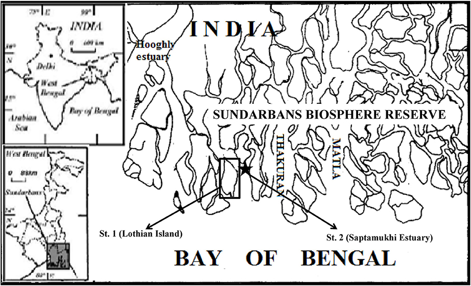
Figure 1. Map showing locations of study area points where Lothian Island and its bordering Saptamukhi river estuary are presented with a sub-set.

Field Sampling, Flux Measurements, and Analytical Methods

Field Sampling

The present study was conducted during June 2010 to December 2012. Sediment and air samples were collected from intertidal mangrove sediments and a watch tower, located at the center of the Lothian Island (21° 42.58′N: 88°18′E), respectively (Figure 1). Water samples were collected in duplicate, on monthly basis from the Saptamukhi estuary along an estuarine stretch of 5 km (with 1 km intervals) near the Lothian Island jetty. Water temperature and pH were recorded in situ using a field thermometer and a portable pH meter (Orion Star A211), with a Ross combination electrode calibrated on the NBS (US National Bureau of Standards) scale (Frankignoulle and Borges, 2011). Reproducibility was ±0.005 pH units. Salinity and dissolved oxygen concentrations in surface and sub-surface waters were measured onboard, following the Mohr-Knudsen and Winkler titration methods, respectively (Grasshoff et al., 1983). Transparency of the water column was measured with a 15 cm diameter secchi disc. Water samples for dissolved inorganic nitrogen (DIN) analyses (e.g., nitrite, nitrate, and ammonia) were filtered in the field through Whatman GF/F filter paper, stored in HDPE bottles, and transported on ice to the laboratory.

Flux Measurements

Analysis of Sediment Samples and Flux Calculations across Sediment-Atmosphere and Sediment-Water Interfaces

Intertidal sediment cores (0–25 cm depth) were collected seasonally from different littoral zones (upper, mid, and lower) on the island using hand-held stainless-steel corers (diameter: 10 cm). Estuarine bottom sediments (sub-tidal) were collected using grab samplers. All sediment samples were sealed in polythene bags and stored on ice during transport to the laboratory.

Cores were sliced in the laboratory (using a N₂-filled glove-bag) at the following 5 cm intervals: 0–5; 5–10; 10–15; 15–20, and 20–25 cm. Sediment redox potential (E_h) was measured immediately using a platinum electrode and Ag/AgCl reference electrode (Fiedler et al., 2003). Wet-sediment samples (both intertidal and sub-tidal) were processed for measurement of CH₄ concentrations. Nitrite concentrations as well as sulfate, acid-volatile sulfide (AVS), and organic carbon percentages were also measured in sediments samples at all depth intervals (Dutta et al., 2013).

CH₄ production rates of collected sediment samples (except 0–5 cm surface layer) were measured using anaerobic sediment incubations. Approximately 10 g of wet sediment were placed in an incubation bottle (1.2 cm i.d. and 10 cm long) fitted with a teflon septum. The bottles were then flushed with high purity N₂ for 1 min. to create completely anaerobic conditions, and incubated in dark at a fixed ambient temperature (i.e., field temperature at that time) for 24 h. At the end of the incubation, a 1 mL gas sample was withdrawn from the headspace through the rubber stopper using a gas-tight glass syringe (Lu et al., 1999). The collected gas sample was then analyzed for CH₄ concentration, based on the purity of nitrogen as blank. CH₄production (in μmol CH₄ m⁻³ wet sediment d⁻¹) was calculated based on CH₄ enrichment in the headspace and volume of the sediment.

CH₄ oxidation was measured for intertidal surface sediment following incubation of wet sediment (~6 cm³) in a 60 mL rubber septum-fitted flask, with a headspace that was spiked with a CH₄ standard (10.9 ppmv; procured from Chemtron Science Laboratories Pvt. Ltd.) (Saari et al., 1997). These flasks were then incubated at ambient temperature (i.e., field temperature) for 4 days in the dark. Gas samples from the headspace were drawn at the onset of incubation and over 24 h intervals until the termination of the experiment, and then analyzed for CH₄ concentrations. CH₄ oxidation was calculated by converting the loss of CH₄ in the headspace with respect to volume of sediment.

During low tide conditions, CH₄ emission rates from the intertidal sediment surface to the atmosphere, were measured using a static perspex chamber method (Purvaja et al., 2004; Dutta et al., 2015b). Basically, the chamber was placed in the sediment for a particular duration and CH₄ emission rate was calculated based on the enrichment of the CH₄ mixing ratio inside the chamber—relative to ambient air. Based on the precision of the air sample measurement method (discussed later), the minimum detectable flux using this chamber method would be 23.30 μmol m⁻² d⁻¹. Advective CH₄ fluxes from intertidal forest sediment to the estuarine water column (F_ISW) were computed according to the method used by Reay et al. (1995): F_ISW = Φ × ν × C; where, Φ = porosity of sediment = 0.58 (Dutta et al., 2013), ν = mean linear velocity = dΦ⁻¹ (d = specific discharge), C = pore water CH₄ concentration in intertidal sediment. Pore-water specific discharge was measured using a traditional, albeit rather “crude” method, which was based on the accumulation of pore water in an excavated pit of known surface area over time (Dutta et al., 2015a). This was performed during extreme low tide conditions on an intertidal flat at 100 m intervals during receding ebb flow. Diffusive CH₄ fluxes were calculated using Fick's law of diffusion (e.g., Sansone and Graham, 2004).

Analysis of Estuarine Water Samples and Water-Atmosphere CH₄ Flux Calculation

Collection and analysis of dissolved CH₄ concentration and CH₄ oxidation rates, in the Saptamukhi River estuarine waters, were performed according to the methods described by Dutta et al. (2013) and Dutta et al. (2015a), respectively; replicates were found to be within 2.30–3.14%. CH₄ fluxes across the air-water interface were calculated based on the wind speed parametization of the gas transfer velocity (k), using the following expression: F_WA = k [CH₄]_observed − [CH₄]_equilibrium] (Liss and Merlivat, 1986). Although, water current speed can play a significant role in generating water-side turbulence (and therefore “k”), as recently reported by Ho et al. (2016), we were not able to include this parameter. A positive value denotes flux from water to the atmosphere and vice versa.

Analysis of Atmospheric Samples, Micrometeorology, and Biosphere-Atmosphere Flux Calculation

Samples for measurement of atmospheric CH₄ mixing ratios were collected on monthly basis using an air sampling bulb, at heights of 10 and 20 m above the forest floor of Lothian Island, and then transported to laboratory for analysis. Two reference gas standards (10.9 and 5 ppmv, procured from Chemtron Science Laboratories Pvt. Ltd.) were run before and after every measurement to check for instrument. Duplicate samples were analyzed periodically and the replicate measurements were found to be within 2–3.2%. Throughout the observation period the measured mixing ratios were corrected for water vapor. Meteorological parameters like air temperature and wind velocity were simultaneously recorded at 10 and 20 m heights above the forest floor of the island using a portable weather station (Model: Davis 7440). Mangrove biosphere-atmosphere CH₄ exchange fluxes (F_BA) were calculated using the following micrometeorological relationship (Barrett, 1998; Ganguly et al., 2008):

${\text{F}}_{\text{BA}}={\text{V}}_{\text{C}}\Delta \chi$

where, Δχ = difference of CH₄ mixing ratio between 10 and 20 m heights, and V_{C =} exchange velocity = 1/(r_a + r_s) (r_a = aerodynamic resistance and r_s = surface layer resistance). Negative flux values indicate influx from the atmosphere to the biosphere, while positive flux indicates an efflux emission from the biophere.

The aerodynamic resistance (r_a) was calculated as follows (Wesely and Hicks, 1977):

${\text{r}}_{\text{a}}=\{\text{ln}(\text{Z}/{\text{Z}}_{\text{o}})-{\Psi }_{\text{c}}\}/{\text{ku}}^{\text{*}}$

where, Z_o is the roughness height, Ψ_c is a correction function for atmospheric stability. Ψ_c was computed as follows (Wesely and Hicks, 1977):

Stable condition: Ψ_c = −5 (Z/L) when 0 < Z/L < 1 (Z = height and L = Obukhov scale length, Z/L = atmospheric stability parameter).

Unstable condition: Ψ_c = exp [0.0598 + 0.39 ln(− Z/L) −0.09{ln (− Z/L)}²] when 0 > Z/L > −1.

The friction velocity (u*) was calculated as follows: u* = k (u₁ − u₂)/ln(Z₂/ Z₁) [k is the Von Karman constant, u₂ and u₁ are wind speeds at two heights, Z₂ and Z₁]

Z_o was determined by plotting the wind profile as lnZ versus u. The slope of the resulting straight line is k/u* and the intercept is lnZ_o. For forest cover, a displacement length (d) equal to 80% of the mean height of the roughness element (mean height of mangrove plant = 10 m) was considered (Panofsky and Dutton, 1984). The scale length (L) was evaluated by the use of Pasquill stability classes A-F (Pruppacher and Klett, 1978) and is related to Z_o (Golder, 1972) as: 1/L = a + b lnZ_o, where “a” ranges between 0.035 and −0.096 and “b” ranges between 0.029 and −0.036.

Surface layer resistance (r_s) for forest cover was calculated as follows (Wesely and Hicks, 1977): k B⁻¹ = 2(K/D_c)^2/3; K = thermal diffusivity of air, D_c = molecular diffusivity = 0.115 (T₂/273)^1.5; T₂ = temperature at 20 m height and B⁻¹ = transfer function.

${\text{r}}_{\text{s}}={\text{B}}^{-1}/{\text{u}}^{\ast }$

Drag coefficient (C_d) at 10 m height was computed as: C_d = r_s/ (ρ × V₁₀₂); ρ = air density and V₁₀ = wind velocity at 10 m height.

Sensible heat flux (H) was calculated as follows (Ganguly et al., 2008): H = ρ_tC_p (T_10m – T_20m)/(r_a + r_s); ρ_t and C_p are density and specific heat of air, respectively.

Height (h) of planetary boundary layer (PBL) was computed as follows (Pal Arya, 2001): h = (0.25 u*)/| F |. F is the Coriolis parameters related to the rotational speed of the earth (Ω) and latitude (Φ) as F=2 Ω sin Φ.

CH₄photo-oxidation rates (P) in the lower forest atmosphere were calculated based on the reaction (CH₄ + OH → CH₃ + H₂O) and equation of P = k [CH₄] [OH] (Dutta et al., 2015b), where, k = rate constant of the reaction between CH₄, and OH = 1.59 × 10⁻²⁰ T^2.84 exp (−978/T) cm³ molecule⁻¹s⁻¹ (Vaghjiani and Ravishankara, 1991), [CH₄] = mean of all CH₄ mixing ratio measurements during the day time at 10 m height in the diurnal cycle, and [OH] = mean of all OH radical concentrations during the day time at 10 m height in the diurnal cycle in molecules cm⁻³. OH radical concentrations were computed using photolysis frequency of O₃ (O₃ mixing ratio in the mangrove forest atmosphere ranged between 14.66 ± 1.88 and 37.90 ± 0.91 ppbv; Dutta et al., 2015b), based on the empirical relation given by Ehhalt and Rohrer (2009).

Analytical Measurements

All CH₄ concentrations were measured according to method described Knab et al. (2009)—whereby, measurement of headspace CH₄ was performed using gas chromatograph (Varian CP3800 GC), fitted with chrompack capillary column (12.5 m × 0.53 mm), and a flame ionization detector (FID); the relative uncertainty for measurments were ± 2.9%.

Sulfate and acid-volatile sulfide (AVS) concentrations of sediment samples were analyzed using standard spectrophotometric methods (Mussa et al., 2009; Simpson, 2011). All DIN concentrations (nitrate, nitrite, and ammonia) were also measured using standard spectrophotometric method (Grasshoff et al., 1983). Replicates were found to be within 2.34–3.15, 2.07–3.69, 1.83–2.74, 3.11–3.87, and 3.24–3.99, respectively, for sulfate, AVS, nitrite, nitrate, and ammonia estimations. Percentage organic carbon (%OC) of dried sediment samples were estimated using a high temperature combustion technique (TOC analyzer, Shimadzu SSM-5000A), which had a mean relative uncertainty of 2.8% (Dutta et al., 2013).

Statisical Methods

All the statistical analyses were performed using Sigma Plot Statistical Software version 11. A simple t-test was used to test for significance acorss different seasons, while multiple regression analyses were used to identify key controlling factors for variability in pore water CH₄ concentrations as well as sediment and water column CH₄ oxidation.

Results and Discussion

Sediment Geochemistry in the Mangroves of Lothian Island

Spatial patterns in sedimentary CH₄ production in the mangrove links significantly with redox potential (E_h). E_h values of mangrove surface sediment varied between −119.8 and −103.2 mV having a mean of −111.4 ± 6.78 mV (Figure 2). Mangrove sediment redox potential values decreased significantly with sediment depth-reaching a minimum at 25 cm (varied between −167.8 and −221.4 mV, mean = −186.7 ± 24.6 mV). These negative redox potential values indicated strong reducing conditions in mangrove sediments; even the oxic surface was not easily detectable. These observed redox condidions, which are highly conducive for anearobic microbial metabolism favors significant production of biogenic trace gases such as N₂O, CH₄, and H₂S in this mangrove system (Dutta et al., 2013). In contrast to the Sundarbans mangrove ecosystem, mangrove sediments of New Caledonia were found to have positive redox potential values, to a sediment depth of 30 cm, with negative E_h values only found in considerably deeper sediments (Deborde et al., 2015). Such extreme differences sediment redox potential across different mangrove systems can typically be attributed to the geological setting (sediment porosity, organic matter supply), ecological factors (floral and faunal activities), hydrologic regime (tidal inundation and flushing). Past work has shown that methanogensis typically occurs at a redox of < −150 mV (Wang et al., 1993) similar to values observed in Lothian Island sediments (at depth of 10–25 cm), consistent with our previous work Dutta et al. (2013). Surface sediment ${\text{SO}}_4^{2-}$–S concentrations ranged from 15.36 to 25.07 mM, with a mean of 20.54 ± 4.89 mM (Figure 3). The range of ${\text{SO}}_4^{2-}$–S concentrations between sediment depths of 20–25 cm was 27.16–27.70 mM, were 1.34 times higher than surface sediment values. Once again, if we compare these ${\text{SO}}_4^{2-}$–S concentrations to the mangrove system in New Caladonia, they are considerably lower (Deborde et al., 2015). One other difference was that in the Lothian Island Sundarbans sediment, ${\text{SO}}_4^{2-}$–S concentrations had a significant decrease only within upper 15 cm depth of sub-surface mangrove sediment consistent with patterns of peak sulfate reduction, with methanogenesis occurring deeper in the sediments (more discussion on this later).

FIGURE 2

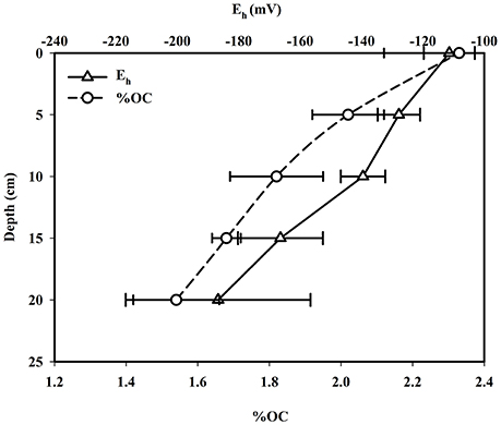
Figure 2. Vertical distributions of E_h and percent OC in mangrove sediment.

FIGURE 3

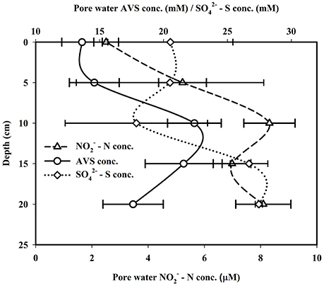
Figure 3. Vertical distributions of pore water ${\text{NO}}_2^{-}$ - N, ${\text{SO}}_4^{2-}$ - S, and AVS concentrations in mangrove sediment.

AVS concentrations in the Lothian Island Sundarbans sediment varied between 13.32 and 13.95 mM with a mean of 13.63 ± 0.32 mM (Figure 3). In contrast to sulfate profiles, downcore AVS concentrations showed distinctly higher values within the 10–15 cm region of the sediment profile. Mangrove surface sediment ${\text{NO}}_2^{-}$–N concentrations varied between 1.61 and 4.14 μM, with a mean of 2.51 ± 1.41 μM. However, downcore ${\text{NO}}_2^{-}$–N concentrations reached a maximum between 10 and 15 cm depth in sediments (varied between 1.99 and 18.53 μM), possibly indicating the dominance of denitrifying bacterial activity at that depth (Figure 3). Percent OC in mangrove surface sediments on Lothian Island varied between 2.1 and 2.51, with a mean of 2.33 ± 0.21 (Figure 2), and decreased in concentration by ~34% at sediments depths of 20–25 cm, where concentrations varied between 1.41 and 1.63%. The %OC measured here was lower than values previously reported by Jennerjahn and Ittekkot (1997) for the mangrove area in the Paraiba do Sul river mouth (4.82%). However, they were within the range of those reported by Bouillon et al. (2004) for mangroves located near Godavari estuary (0.6–31.7%), near the Indian and southwest coast of Srilanka. The decreasing trend of %OC coupled with decreasing redox potential across deep mangrove sediment indicates significant OC mineralization by anaerobic microbial respiration.

CH₄ Production Rates in Sediment

While only marginal CH₄ production (215–1,176 μmol CH₄ m⁻³ wet sediment d⁻¹) was observed in sediments between 5 to 10 cm in depth, a significant [p (= 0.02) < 0.05] increase (2,089 to 4,033 μmol CH₄ m⁻³ wet sediment d⁻¹) was observed at sediment depths of 10 to 15 cm (Figure 4). This trend of increasing CH₄ production rates with sediment depth continued even deeper in mangrove sediments with increases between 2,919 to 5,903 and 4,290 to 7,353 μmol CH₄ m^-3 wet sediment d⁻¹, respectively, for depth of 15 to 20 cm [p (= 0.32) > 0.05] and 20 to 25 cm [p (= 0.31) > 0.05]. The depthwise (D) variability of CH₄ production rates ([CH₄]_PI) in the intertidal sediment column was examined using the following logarimetric equation:

${[C{H}_4]}_{\text{PI}}=3547\text{ lnD}-5045({\text{R}}^2=0.99)$

The production rates measured for this study site varied between 215 and 7,353 μmol CH₄ m⁻³ wet sediment d⁻¹, mean = 3,547 ± 2,205 μmol CH₄ m⁻³ wet sediment d⁻¹, and were within the range reported for pristine mangrove forests at Balandra, Mexico (Strangmann et al., 2008). While we did not measure CH₄ in the upper 0 to 5 cm in this study, due to the low methanogenic and intense methanotrophic activities in that layer, these rates are likely an underestimate-but were still quite high. However, in the bordering Saptamukhi estuarine system near our study site, CH₄production rate in the top 5 cm of sub-tidal sediment varied between 18.72 and 85.74 μmol CH₄ m⁻³ wet sediment d⁻¹, with a mean of 48.88 ± 26.04 μmol CH₄ m⁻³ wet sediment d⁻¹.

FIGURE 4

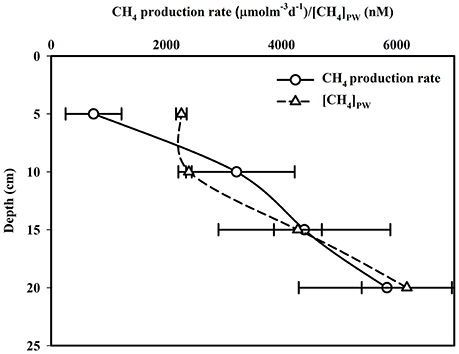
Figure 4. Vertical distributions of CH₄ production rates and pore water CH₄ concentrations at intertidal mangrove sediment.

Seasonally, mangrove sediment CH₄ production rates were higher [p (= 0.21) > 0.05] in post-monsoon (4,616 ± 2,666 μmol CH₄ m⁻³ wet sediment d⁻¹) compared to pre-monsoon (2,378 ± 1,799 μmol CH₄ m⁻³ wet sediment d⁻¹) seasons. The higher post-monsoon CH₄ production rate may be attributed to the presence of high mangrove leaf litter-fall at this time (58.79 g dry wt C m⁻² month⁻¹; Ray et al., 2011), which likely mediated by the supply of labile organic matter in these sediments- supporting higher CH₄ production. In contrast, higher salinity conditions during pre-monsoon may have partially inhibited sediment CH₄ production rate. For example, Marton et al. (2012) also reported lower CH₄ production rates during high salinity conditions. Other work in tidal mangrove forests have shown that intrusion of high salinity waters results in higher pore—water salinities, along with availibility of terminnal electron acceptors (e.g., ${\text{NO}}_3^{-}$, ${\text{SO}}_4^{2-}$)—which constrain CH₄ production (Craft et al., 2009; Larsen et al., 2010).

Sub-tidal sediment in post-monsoon season had significantly [p (= 0.03) < 0.05] higher CH₄ production rates (77.06 ± 12.27 μmol CH₄ m⁻³ wet sediment d⁻¹) compared to pre-monsoon conditions (21.28 ± 3.63 μmol CH₄ m⁻³ wet sediment d⁻¹). These was a ~35.25% higher OC supply to the sub-tidal sediment surface during post-monsoon (2.21 ± 0.69%) compared to pre-monsoon (1.56 ± 0.72%), which likely contributed to the observed oxygen draw-down which favored higher CH₄ production.

Utilization of Organic Carbon and Linkages to Methanogenesis

Methanogens can only utilize a limited number of substrates and with the major pathways being (I) fermentation of acetate, commonly referred to as acetoclastic methanogenesis (AM) (Equation 1), and (II) acetate oxidation (Equation 2), where CO₂ is reduced with H₂ (hydrogenotrophic methanogenesis [HM]) (Equation 3) (Zinder, 1993; Mayumi et al., 2013). The aforementioned equations are shown below:

$\begin{array}{ll}{\text{CH}}_3{\text{COO}}^{-}+{\text{H}}^{+}={\text{CH}}_4+{\text{CO}}_2& (1)\end{array}$

$\begin{array}{ll}{\text{CH}}_3{\text{COO}}^{-}+{\text{H}}^{+}+{\text{2H}}_2\text{O}={\text{4H}}_2+{\text{2CO}}_2& (2)\end{array}$

$\begin{array}{ll}{\text{4H}}_2+{\text{CO}}_2={\text{CH}}_4+{\text{2H}}_2\text{O}& (3)\end{array}$

Mayumi et al. (2013) calculated change in Gibbs free energy (ΔG°) values for the aforementioned reactions in well-controlled CO₂-injected microcosms. This work showed that acetate oxidation, under these microcosm conditions, was endergonic-indicating a predominance of AM over the HM in a CO₂-rich environment. Moreover, Lessner (2009) reported that ~70% of biologically-produced CH₄ originated from the conversion of the methyl group of acetate to CH₄. Thus, considering the CO₂-rich character of the Sundarban mangrove environment (Biswas et al., 2004), we speculate that AM likely predominated in these sediments. If we make this assumption, the stoichiometric equation of acetoclastic methanogenesis (Equation 1) would require the utilization of 2 moles of OC per mole of CH₄ production. Along with production of CH₄, the reaction also produces one mole of CO₂ as by-product. Using the above equations, we calculated that in the intertidal sediment (from 0 to 25 cm depth), 4,966 μmol m⁻³ d⁻¹ of OC was transformed through an AM pathway producing both CH₄ and CO₂ as 2,483 μmol m⁻³ d⁻¹. Similarly in the estuarine bottom sediment, adjacent to the island, 68.33 μmol m⁻³ d⁻¹ of OC was transformed through the AM pathway producing 34.22 μmol m⁻³ d⁻¹ of CH₄ and 34.22 μmol m⁻³ d⁻¹ of CO₂. The release of CH₄, and CO₂ as by-products, possibly enhancing potential regional effects on climate change. However, mangroves are also well-known to be blue carbon habitats, which sequester and store CO₂ (Bouillon et al., 2008; Alongi, 2012). Thus, further work is needed to establish the overall role of these mangroves as net sinks or sources of greenhouse gases. Finally, although we did not examine the role of sulfate reduction in this study, based on the relatively low %OC in these mangrove sediments (Prasad et al., 2017), it is likely to be another very important anaerobic process for sedimentary OC processing in the Sundarbans mangrove ecoystem.

Pore-Water CH₄ Levels and its Fluxes to the Adjacent Saptamukhi River Estuary

Pore-water CH₄ concentrations in intertidal mangrove sediments of Lothian Island were relatively constant within the 10 to 15 cm sediment layers (varied between 1,881 and 2,429 nM), and then abruptly [p (= 0.001) < 0.05] increased to concentrations of 3,804 and 4,542 nM between 15 and 20 cm-with further significant increases [p (= 0.02) < 0.05] to 5,274 and 6,670 nM between 20 and 25 cm (Figure 4). On seasonal basis, mean pore-water CH₄ concentrations in intertidal sediments were higher [p (= 0.69) > 0.05] in post-monsoon (3,639 ± 1,949 nM) compared to pre-monsoon season (3,204 ± 1,325 nM) (Dutta et al., 2015a). Considering pore-water CH₄ concentration ([CH₄]_PW) as a dependent variable relative to other independent parameters measured (E_h, [${\text{NO}}_2^{-}$–N], [${\text{SO}}_4^{2-}$–S], [AVS] and %OC), a multiple regression analysis ([CH₄]_PW = 0.03 − 0.0308 E_h − 1.08[%OC] + 0.0691 [${\text{SO}}_4^{2-}$–S] − 0.0459[AVS] + 0.0034 [${\text{NO}}_2^{-}$–N]; R² = 93.1%, F = 21.71, p < 0.001, n = 28) revealed a significant correlation between [CH₄]_PW and E_h (p = 0.017)—but not with others. This suggests the potential impact of sediment redox potential on the variability of mangrove sediment pore-water CH₄ concentrations. Mean sub-tidal sediment pore-water CH₄ concentrations were significantly higher in pre-monsoon (3,980 ± 1,227 nM) than in post-monsoon conditions (2,770 ± 1,039 nM) (Dutta et al., 2015a), which followed a similar seasonal trend for intertidal sediments. Overall, sediment pore waters in the intertidal mangrove sediments of Lothian Island were ca. 53.4 times more supersaturated than the adjacent estuarine sediments. This clearly indicates a significant source CH₄ to the estuarine CH₄ sediment pool, via advective (ranged between 115.81 ± 31.02 and 199.15 ± 47.89 μmol m⁻² d⁻¹; Figure 5) and diffusive fluxes (ranged between 7.06 ± 1.95 and 10.26 ± 2.43 μmol m⁻² d¹; Figure 6) (Dutta et al., 2015a). Unfortunately, to the best of our knowledge no estimates have been made on advective CH₄ fluxes from intertidal mangrove to Saptamukhi River estuarine system. It should be noted that these are the the first reported measurments of advective CH₄ fluxes from Indian Sundarbans, albeit using a traditional rather “crude” method. Although, our estimated pore water specific discharge rates (3.60–5.76 cm d⁻¹) were in the range of that measured for other mangrove regions located at temperate and tropical regions (2.10–35.50 cm d⁻¹; Tait et al., 2016) by combined natural tracer Radon (²²²Rn) with hydrodynamic models but as such, more accurate measurements are needed in near future to better constrain such measurements in the this globally-important ecosystem.

FIGURE 5

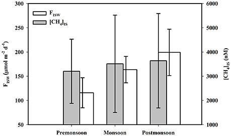
Figure 5. Seasonal variations of mangrove sediment pore water CH₄ concentration ([CH₄]_IS) and its advective flux to estuary (F_ISW)

FIGURE 6

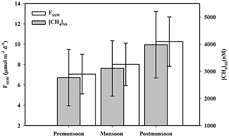
Figure 6. Seasonal variations of sub-tidal sediment pore water CH₄ concentration ([CH₄]_SS) and its diffusive flux to estuary (F_SSW).

When compared to a temperate system, diffusive CH₄ fluxes from sub-tidal sediment of the Saptamukhi estuary were comparable to those found in the Arcachon tidal lagoon (France) (11.97 μmol m⁻² d⁻¹; Deborde et al., 2010). Similarly, our diffusive CH₄ fluxes were also higher than in the Yangtze temperate estuary, China (1.7–2.2 μmol m⁻² d⁻¹; Zhang et al., 2008), yet lower than White Oak river estuary, in northern California (17.1 μmol m⁻² d⁻¹; Kelley et al., 1990). While such cross-system comparisons are frought with the complexity of regional differences in ecological and physicochemical drivers of fluxes, we provide them for a simple geographic perspective here. Nevertheless, we can conclude that in the Indian Sundarbans fluxes measured during post-monsoon period were higher compared to pre-monsoon conditions, but were only significant for advective fluxes [p (= 0.0006) < 0.05] —not for diffusive fluxes [p (= 0.21) > 0.05]. The peak post-monsoon advective CH₄ flux may be due to maximal intertidal sediment pore water CH₄ concentrations, as well as pore water specific discharge (5.76 cm d⁻¹). Peak diffusive CH₄ flux may be attributed to maximal sub-tidal sediment pore water CH₄concentrations, which resulted in a greater CH₄ concentration gradient at sediment-water interface.

CH₄ Oxidation and Emission at/from Mangrove Surface Sediment

Mean surface sediment CH₄ oxidation rates (1.76 ± 0.34 mg m⁻² d⁻¹) measured in the Lothian Island mangrove forest were within the range of that reported by Bradford et al. (2001) and Jang et al. (2006). The mean peak pre-monsoon CH₄ oxidation rate (2.149 ± 0.16 mg m⁻² d⁻¹; Figure 7) are likely linked with maximum soil surface temperatures. Seasonal CH₄ exchange across mangrove sediment–atmosphere interface in Lothian Island mangroves revealed an annual mean flux of 452 ± 126 μmol m⁻² d⁻¹ (Figure 7), indicative of a net source of CH₄ from mangrove sediments to the atmosphere. These fluxes were within the range of those reported by Purvaja et al. (2004) in the Pichavaram mangrove, located at the northern end of the Cauvery delta, India, and along the coast of Puerto Rico (Sotomayor et al., 1994). Soil temperatures and salitinties have been show to have a significant impact on CH₄ emissions (F_SA) from mangroves (Bartlett et al., 1987; Lekphet et al., 2005). Lothian Island mangroves soil temperature and pore water salinity ranged between 18.25 ± 0.22 and 28.36 ± 1.02°C (t) and 22.55 ± 0.31 and 28.88 ± 0.13 (s), respectively. Both soil temperature and salinity were maximal during pre-monsoon and minimal during post-monsoon seasons, respectively. “F_SA” was best fitted linearly with “t” (R² = 0.35, F = 5.33, p = 0.041, n = 12), however, a second order polynomial relationship with “s” (R² = 0.77, F = 7.71, p = 0.029, n = 12), indicated a cumulative effect of temperature and salinity on variability of sediment CH₄ emission fluxes. A similar effect was previously reported in Ranong Province mangrove area, Thailand (Lekphet et al., 2005) and in a salt marsh at Queen's creek (Bartlett et al., 1987).

FIGURE 7

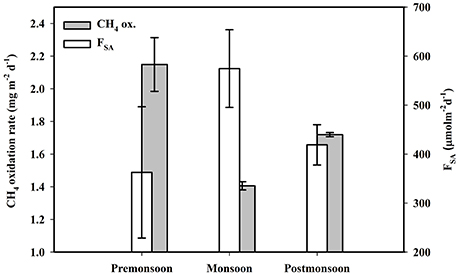
Figure 7. Seasonal variations of mangrove surface sediment CH₄ oxidation and CH₄ emission (F_SA) across mangrove sediment-atmosphere interface of Lothian Island.

In Lothian Island mangroves, we observed higher spatial variability on CH₄ emissions (432–761 μmol m⁻² d⁻¹) in the upper littoral zone compared to mid and lower littoral zones. This was likely due to the higher pneumatophore density in that region (42 number m⁻²) and the associated plant-mediated diffusion of CH₄ through them (Dutta et al., 2013). This further supports the role of plant-mediated transport of CH₄ across the sediment atmosphere interface in aquatic system (Chanton and Dacey, 1991; Laanbroek, 2010; Bridgham et al., 2013). In fact, a significant correlation was found between “F_SA” with both pneumatophore (P_no) and bioturbation (B_o) densities, with positive correlation with pneumatophore (F_SA = 400.13 + 0.56 P_no; R² = 81.9%, F = 6.94, p = 0.032, n = 20) and negative with bioturbation (F_SA = 444.38–0.028 B_no; R² = 61.9%, F = 5.94, p = 0.041, n = 20). The positive correlation between sediment CH₄ emission flux with pneumatophore density via plant-mediation, and negative correlation via bioturbation e.g., burrowing crabs (Kristensen and Alongi, 2006), reflect the complex and changing dynamics of plant-and-animal populations on intertidal sediment-atmosphere CH₄ emission fluxes.

Estuarine CH₄ Biogeochemistry

Physicochemical Properties of the Saptamukhi River Estuary

Physicochemical parameters of the Saptamukhi River estuarine waters are presented on seasonal basis in Figures 8, 9. For both temperature and salinity, the values were highest during the pre-monsoon and lowest during the post-monsoon (for temperature) and monsoon (for salinity) months. The lack of variability between estuarine surface and sub-surface water temperature and salinity clearly indicated the presence of a well-mixed water column (Dutta et al., 2015a). Seasonal differences of pH were not significant and ranged between 8.10 ± 0.03 and 8.17 ± 0.16. Dissolved oxygen (DO) concentrations in estuarine surface and sub-surface waters were high (0.19 ± 0.023 to 0.23 ± 0.036 and 0.17 ± 0.001 to 0.19 ± 0.025 mM, respectively; Figure 8), and DO % of saturation ranged from 94.8 to 99.3. These high oxygen values reflect a well-mixed oxygenated water column, that should restrain most anaerobic microbial metabolism of organic matter within estuarine water column. However, it should also be noted that CH₄ production in the isolated anoxic microhabitats of sinking particulate organic matter (POM), in well-oxygenated water column, have been observed in the open ocean (see Reeburgh, 2007).

FIGURE 8

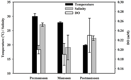
Figure 8. Seasonal variations of estuarine surface water temperature, salinity, and DO conc.

FIGURE 9

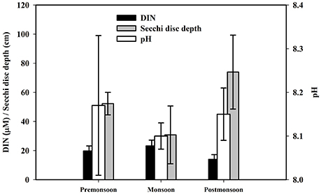
Figure 9. Seasonal variations of estuarine surface water DIN conc., pH and secchi disc depth.

Distribution of Dissolved CH₄

Previous studies have shown that CH₄ concentrations of the Saptamukhi River estuarine surface and sub-surface waters ranged from 54.20 ± 5.06 to 90.91 ± 21.20 and 47.28 ± 12.85 to 67.97 ± 33.12 nM (Table 1), respectively (Dutta et al., 2015a). The concentrations measured for this tropical mangrove-dominated estuary (Figure 10) were within the range of that reported for other tropical estuaries located at west (113 ± 40 nM) and east (27 ± 6 nM) coast of India, such as Luper (5.2–59 nM) and Saribus (3.7–135 nM), as well as estuaries located in northwestern Borneo (Muller et al., 2016; Rao and Sarma, 2016). Seasonally, estuarine surface water CH₄ concentrations during post-monsoon (90.91 ± 21.20 nM) were significantly higher [p (= 0.01) < 0.05] compared to pre-monsoon (54.20 ± 5.06 nM) conditions. This was likley due to the cumulative effects of maximum CH₄-rich pore water influx from adjacent intertidal mangrove sediments to the estuary as well as minimal CH₄ oxidation (will be discussed later) within these estuarine waters during post-monsoon conditions. Estuarine CH₄ concentrations showed a significantly negative correlation with salinity (pre-monsoon: R² = 89.1%, F = 49.15, p < 0.001, n = 8; monsoon: R² = 95.2%, F = 120.12, p < 0.001, n = 8; post-monsoon: R² = 75.8%, F = 18.83, p = 0.005, n = 8), indicating that salinity is the major governing factor for variability of CH₄ concentration in this estuary. This same pattern has been shown for other tropical and sub-tropical estuaries (Upstill-Goddard et al., 2000; Middelburg et al., 2002; Biswas et al., 2007; Zhang et al., 2008). Moreover, Dutta et al. (2015a) established that much of the dissolved CH₄ in the estuarine system of Sundarbans was from exogenous sources.

TABLE 1

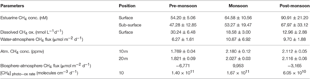
Table 1. Seasonal variation (mean ± SD) of estuarine and atmospheric CH₄ concentrations, oxidation and exchanges across different interfaces.

FIGURE 10

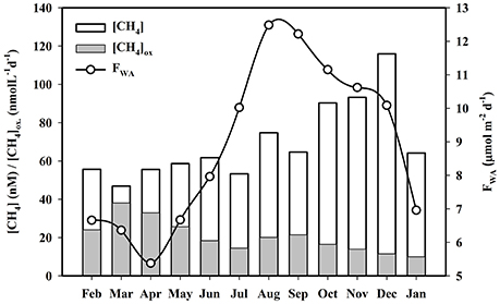
Figure 10. Monthly variations of estuarine dissolved CH₄ conc., CH₄ oxidation, and air-water CH₄ exchange flux (F_WA)

Dissolved CH₄ Oxidation in Saptamukhi River Estuary

The Saptamukhi River estuarine water column is a well-oxygenated system that favors the activity of methanotrophs. Other studies have shown the mean dissolved CH₄ oxidation rate in these estuarine surface waters to be 20.59 nmol L⁻¹ d⁻¹, and varies between 12.96 ± 2.88 and 30.24 ± 6.48 nmol L⁻¹ d⁻¹ (Table 1) (Dutta et al., 2015a). Seasonally, CH₄ oxidation rates during the pre-monsoon period were significantly [p (= 0.002) < 0.05] higher than post-monsoon periods (Figure 10). Aquatic CH₄ oxidation has been shown to be significantly impacted by other physicochemical parameters such as temperature (thermal), salinity (tonicity), oxygen (oxidative), DIN (nutrient), and turbidity (surface). In the case of turbidity, estuarine methanotrophs, associated with suspended particulate matter, may be more effeicient in oxidizing CH₄ in the water column (Abril et al., 2007). Considering dissolved CH₄ oxidation rate ([CH₄]_DOX) as dependent variable, relative to other independent parameters measured (T, S, DO, [DIN] and S_D), a multiple regression analysis ([CH₄]_DOX = −61.8+0.732 T + 1.97 s + 7.24 DO − 0.456 DIN - 0.290 S_D; R² = 90.8%, F = 11.91, p = 0.005, n = 12) revealed a significant correlation between [CH₄]_DOX with only S (p = 0.002), DO (p = 0.037) and S_D (p = 0.019), but not with others. This further supports the need to examine broader spectrum and variability of drivers on CH₄ oxidation in these complex estuarine waters.

Saturation Percentage of CH₄ and Air-Water CH₄ Exchange

Percent saturation of dissolved CH₄ in the Saptamukhi River estuary ranged from 2,483 ± 950 to 3,525 ± 1,054, indicating that estuarine waters were supersaturated in CH₄, highly conducive for CH₄ efflux across the water-atmosphere interface. Seasonal variability in CH₄ exchange across air-water interface of this estuary are shown in Figure 10 (Dutta et al., 2015a). Flux values calculated during the monsoon period (10.67 ± 6.92 μmol m⁻² d⁻¹) were significantly higher [p (= 0.007) < 0.05] compared to pre-monsoon conditions (6.27 ± 1.61 μmol m⁻² d⁻¹) (Table 1). Air-water CH₄ fluxes were in the range of that calculated for other tropical estuaries, like the Hooghly estuary (0.88–148.63 μmol m⁻² d⁻¹) and Yangtze River estuary (6–25 μmol m⁻² d⁻¹) (Biswas et al., 2007; Zhang et al., 2008). The lowest CH₄ fluxes during pre-monsoon season were likely attributed to the coupled impact of low wind speeds, resulting low gas transfer velocities, as well as low dissolved CH₄ concentrations in surface waters. Estimated CH₄ flux values estimated for the Saptamukhi River estuary showed asignificant correlations with water temperature and salinity (water temperature: R² = 61%, F = 6.71, p = 0.029, n = 24; salinity: R² = 54%, F = 5.31, p = 0.037, n = 24), indicating cumulative effects of temperature and salinity on CH₄ emission fluxes (Dutta et al., 2015a). On an annual basis, the mean CH₄ emission flux across the water-atmosphere interface was 8.88 μmol m⁻² d⁻¹, indicating that the estuary acted as a source of CH₄ to the regional atmosphere during this study period.

Atmospheric CH₄ Dynamics at Lothian Island in the Indian Sundarbans

Micrometeorology and Atmospheric CH₄ Mixing Ratio

Previous work has shown that the lowest air temperatures and wind velocities, on Lothian Island, occurred during the post-monsoon season and were at their maximum during pre-monsoon conditions (Dutta et al., 2015b). Friction velocity (u*), which controls stability of the atmosphere (e.g., atmospheric turbulence), varied between 0.01 and 1.2 m s⁻¹. PBL heights over the mangrove forest atmosphere (702.45 to 936.59 m), and were highest and lowest during pre-monsoon and monsoon periods, respectively. The values of drag coefficient (0.16–0.39) and roughness height (varied between 1.63 ± 1.02 and 3.77 ± 3.01 m) also followed the same seasonal trends.

Dutta et al. (2015b) measured atmospheric CH₄ mixing ratios at 10 and 20 m heights in the mangrove forest on Lothian Island (Figure 11). The lowest atmospheric CH₄ mixing ratios were observed during pre-monsoon (at both 10 and 20 m heights) season, while maximum ratios were found during monsoon and post-monsoon periods for 10 m and 20 m heights, respectively (Table 1). The significantly higher CH₄ concentrations in air [p (= 0.001) < 0.05] at 10 m height during monsoon season, compared to pre-monsoon, may be attributed to peak monsoon CH₄ emissions from sediments and aquatic surfaces, which primarily contribute to lower atmospheric CH₄ pool. We have also shown peak CH₄ concentrations in air occurring during early morning, which may be attributed to CH₄ accumulation within a stable boundary layer during that period (Dutta et al., 2015b). Concentrations of CH₄in the lower atmosphere have been shown to decrease with advancing daylight due to increases in atmospheric turbulence-which tends to break-up a stable boundary layer (Mukhopadhyay et al., 2002). The atmospheric stability parameter (Z/L) and CH₄ mixing ratio (at 10 m height) were significantly correlated (R² = 74.8%, p < 0.001, F = 29.73, n = 30), this further supports that micrometeorology plays an important role in the variability of CH₄ mixing ratio in the lower atmosphere of mangrove forests in the Indian Sundarbans (Dutta et al., 2015b).

FIGURE 11

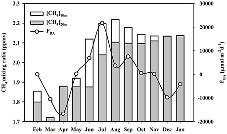
Figure 11. Monthly variations of atmospheric CH₄ mixing ratio at 10 and 20 m heights and biosphere-atmosphere CH₄ exchange flux (F_BA).

Exchanges of CH₄ across Biosphere–Atmosphere Interface

On an annual basis, atmosphere CH₄mixing ratios measured at 10 m height over Lothian Island were 2% higher compared to 20 m, indicating CH₄exchanges across the biosphere–atmosphere interface that were modulated by atmospheric turbulence. Our previous work (Dutta et al., 2015b) has shown monthly CH₄ exchange fluxes of across mangrove biosphere–atmosphere interface (Figure 11), that have maximal fluxes during monsoon and minimal during post-monsoon periods (Table 1). These values also confirmed that mangroves were a CH₄ source to the upper atmosphere during the monsoon period (flux values positive), when Δχ was a significantly positive sink, in contrast to periods during pre-and post-monsoon seasons (flux values negative), when Δχ was negative. During the observation period, the mean mangrove biosphere-atmosphere CH₄ exchange flux was estimated to be 5.5 μmol m⁻² d⁻¹, which indicated that on an annual basis these mangroves were dominant sources of CH₄ to the upper atmosphere. The mean compensation point, where the net biosphere-atmosphere CH₄ flux is zero, was found to be 1.997 ppmv. Sensible heat flux (H), which moderately controls atmospheric transport of energy and mass, was significantly correlated with biosphere–atmosphere CH₄flux (F_BA). This was defined by a second order polynomial relationship (R² = 0.53, F = 7.72, p = 0.002, n = 12), further supporting the significant influence of sensible heat flux on the variability of biosphere-atmosphere CH₄ exchange fluxes (Dutta et al., 2015b).

Atmospheric CH₄ Photo-Oxidation

On annual basis, the mean daytime CH₄ mixing ratio was estimated to be 1.03 times lower than at nighttime; this variability is expected to be cumulatively governed by photo-oxidation and diurnal changes of PBL height. Dutta et al. (2015b) reported an insignificant correlation between daytime and nighttime CH₄ mixing ratios with PBL height (ΔCH₄ = −0.0118ΔPBL + 0.3045; R² = 16.2%, F = 0.321, p = 0.987, n = 12), and for the first time, showed the presence of CH₄ photo-oxidation within this tropical mangrove forest atmosphere. More specifically, this work reported CH₄ photo-oxidation rates in the forest atmosphere that varied between 6.05 × 10¹⁰ and 1.67 × 10¹¹ molecules cm⁻³ d⁻¹, and were maximal and minimal during monsoon and post-monsoon periods, respectively (Table 1). The significantly higher monsoon CH₄ photo-oxidation rate [p (= 3.2 × 10⁻⁷) < 0.05] compared to post-monsoon, may be attributed to the combined effect of maximum CH₄ influx to atmosphere through emissions across sediment-atmosphere and water-atmosphere interfaces-as well as high UV indices and UV erythermal doses of irradiance that occur during this period in subtropical latitudes (Panicker et al., 2014). When considering a mean day light period of 12 h and that 6.023 × 10²³ molecules equals to 1 mole or 16,000 mg CH₄, the mean CH₄ photo-oxidation rate to the atmosphere in this tropical mangrove-dominated island was calculated to be 3.25 × 10⁻⁹ mg cm⁻³ d⁻¹.

Quantitative CH₄ Budget for Sundarbans Mangrove Ecosystem

A box model was developed on the biogeochemical cycling of CH₄—as well as a quantitative CH₄ budget for the Sundarbans mangrove ecosystem (Figure 12). In the model different subecosystems are designated as separate reservoirs. The CH₄ pool in each reservoir and exchange fluxes between different reservoirs are presented on an annual mean basis. The major outputs from the box model are described below.

FIGURE 12

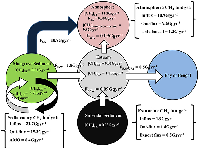
Figure 12. Biogeochemical CH₄ cycling at Indian Sundarbans. Here, [CH₄]_ST = CH₄ storage, [CH₄]_PR = CH₄ production, [CH₄]_OX = CH₄ oxidation, F_ISW = advective CH₄ flux, F_SSW = diffusive CH₄ flux, F_SA = mangrove sediment-atmosphere CH₄ flux, F_BA = mangrove biosphere-atmosphere CH₄ flux, and F_EXPORT = CH₄ export flux from estuary to northern Bay of Bengal.

Mangrove/Intertidal Sediment Methane Budget

Total annual CH₄ production in Sundarbans mangrove sediment, within an intertidal sediment depth of 25 cm, was estimated to be 21.7 Gg year⁻¹, with a daily rate of 3,547 μmol m⁻³ d⁻¹. The CH₄ sediment reservoir pool was 0.03 Gg, with a mean pore-water CH₄ concentration 3,451 nM. Pore water was ~55 times more supersaturated than adjacent estuarine waters (63.0 nM). This suggests that during low tide, depending upon the hypsometric gradient, there is a significant out-flux of CH₄-rich pore water from the intertidal mangrove sediments to estuary, via advective transport. Extrapolating a mean advective CH₄ influx from mangrove sediment to the adjacent estuary (159.5 μmol m⁻² d⁻¹) for entire intertidal area of Indian Sundarbans (45% of total forest area; http://www.sundarbanbiosphere.org/html_files/sunderban_biosphere_reserve.htm), we estimate that about 8.2% of the total mangrove sediment produced CH₄ is advectively transported to the adjacent estuarine system, with ~12.4% undergoing oxidation at sediment surface by methanotrophs. Total annual CH₄ emission, from intertidal mangrove sediment to the forest atmosphere, was estimated to be 10.8 Gg year⁻¹ (~49.6% of total produced CH₄ in sediment), with a mean daily rate of 7.1 mg m⁻² d⁻¹. When examining the ratio of [sediment emission]: [aerobic oxidation]: [advective flux], which computes to 6.05:1.51:1, it reveals that CH₄ emission is major CH₄ removal mechanism in these intertidal mangrove sediments. Excess CH₄ remaining ([ΔCH₄]_S) in these mangrove sediments, beyond the aforementioned “sink” mechanisms, was computed as follows:

[ΔCH₄]_S = Total CH₄ production − Total outflux (sediment emission + aerobic oxidation + advective flux). When using this equation, we find sink value [ΔCH₄]_S of 6.4 Gg year⁻¹. This estimated value reflects the removal of CH₄, via anaerobic methane oxidation (AMO), within sub-surface mangrove sediments, that were not considered in this study.

Sub-Tidal Sediment CH₄ Budget

Total CH₄ production at the 0–5 cm depth of sub-tidal sediment was 0.03 Gg year⁻¹, with a mean of 48.88 μmol m⁻³ d⁻¹. Mean sub-tidal sediment pore-water CH₄ concentration was 3,286 nM; which was ~ 52.1 times supersaturated, compared to overlying estuarine water CH₄ levels. This supports the notion of diffusive CH₄ transport mechanism from sub-tidal sediments to the overlying estuary. On annual basis total diffusive CH₄ influx from sub-tidal sediment to the overlying estuary was 0.09 Gg, with a mean of 8.4 μmol m⁻² d⁻¹.

Estuarine CH₄ Budget

The total CH₄ input to the Saptamukhi River estuary (by both advectice and diffusive transport) was 1.8 Gg year⁻¹. The ratio between advective and diffusive CH₄ flux was 20:1, indicating that advective CH₄ flux from intertidal mangrove sediments was the dominant driver in the buildup of the estuarine CH₄ pool. The estuary stands as a reservoir pool of 0.01 Gg CH₄, having a mean concentration of 63.0 nM. An estimated 74.5% of total CH₄ supplied to the estuary was removed from the estuarine system-via microbial oxidation, with only 5.0% lost by an air-water CH₄ exchange flux. The ratio between microbial oxidation and air-water CH₄ exchange flux was 14:1, indicating microbial oxidation was the principal CH₄ removal pathway in this estuary. Mean turnover time of CH₄ in the water column relative to oxidation and emission was 3.7 days. After oxidation and emission, excess CH₄ left ([ΔCH₄]_E) in the estuarine system was computed as:

$\begin{array}{l}{[\Delta {\text{CH}}_4]}_{\text{E}}=\text{Total influx }(\text{Advective}+\text{Diffusive})\\ -\text{ Total outflux }(\text{microbial oxidation}\\ +\text{ estuarine emission})\end{array}$

Using the equation, [ΔCH₄]_E was computed as 0.5 Gg year⁻¹, which is estimated CH₄ exported to the adjacent continental shelf region, thereby enriching the CH₄ pool in northern Bay of Bengal.

Atmospheric CH₄ Budget

The total annual CH₄ influx for Sundarbans mangrove ecosystem, via mangrove sediment and estuarine emissions, was 10.9 Gg year⁻¹, of which 99.1% was from sediments. Atmospheric CH₄ mixing ratios at 10 and 20 m heights in the forest atmosphere were 2.03 and 1.98 ppmv, respectively having mean of 2 ppmv. Extrapolating over entire Sundarbans, up to the mean PBL height (811.7 m), the atmosphere stands as a reservoir pool of 11.2 Gg CH₄. The annual mean mangrove biosphere-atmosphere CH₄ exchange flux was estimated to be 5.38 μmol m⁻² d⁻¹. However, when extrapolated for entire forest area it was found that only 2.75% of total annual CH₄influx to the forest atmosphere was transported to the upper forest atmosphere. Moreover, ~85% of total annual CH₄ influx to the forest atmosphere experienced photo-oxidation within the atmospheric boundary layer of Sundarbans, with a mean rate of 3.25 × 10⁻⁹ mg cm⁻³ d⁻¹. Excess CH₄ that was from the forest atmosphere ([ΔCH₄]_A) beyond the photo-oxidation and biosphere-atmosphere fluxes was calculated as follows:

$\begin{array}{l}{[\Delta {\text{CH}}_4]}_{\text{A}}=\text{Total influx }(\text{estuarine emission}\\ +\text{ sediment emission})\\ -\text{ Total outflux}(\text{photo-oxidation}\\ +\text{ biosphere-atmosphere flux})\end{array}$

Using this mass balance equation [ΔCH₄]_A, we estimated that 1.3 Gg year⁻¹ enriches the regional atmospheric CH₄ mixing ratio and further contributes to regional climate change scenarios. The impact of these gases need to be considered as a delineated reservoir, within the context of a regional climate and atmospheric boundary layer height (ABL) (mean height = 811.7 m; Dutta et al., 2015b). Considering a radiative forcing efficiency of CH₄ in the atmosphere as 3.7 × 10⁻⁴ W m⁻² ppb⁻¹ (https://www.ipcc.ch/publications_and_data/ar4/wg1/en/ch2s2-10-2.html), [ΔCH₄]_A in this mangrove forest atmosphere resulted 0.11 Wm⁻² year⁻¹ of radiative forcing to the regional atmosphere.

Conclusions

In intertidal mangrove sediment column CH₄ production rate, down to depth of 25 cm in the sediments, was estimated to be 21.75 Gg year⁻¹ with a mean pore water CH₄ concentration was 3,541 nM. CH₄ emission across intertidal sediment—atmosphere interface acted as major sink for the CH₄ produced in intertidal sediments over surface layer CH₄ oxidation and advective CH₄ transport to Saptamukhi River estuary. The estuary, which was well-oxygenated, which constrained methanogenesis within estuarine water column, where dissolved CH₄ was considered to be entirely exogenous in nature. Advective CH₄ flux, which was 20 times higher than diffusive flux, was the major source for CH₄ to the estuary. CH₄ oxidation which is 14 times higher than the water-atmosphere exchange, was considered the principal CH₄ removal mechanism in this estuary. On an annual basis, total CH₄ emissions from sediments and waters of the Sundarbans mangrove biosphere was 10.9 Gg of which sediment contributed principally 99.1%. Compared to total CH₄ supply to the forest atmosphere, about 85% photo-oxidized within atmospheric boundary layer of Sundarbans while 2.75% is transported to the upper atmosphere through mangrove biosphere-atmosphere CH₄ exchange flux. Based on our proposed CH₄ budget the mangrove forest atmosphere resulted in a radiative forcing 0.11 Wm⁻² year⁻¹ to the regional atmosphere.

Author Contributions

MD and SM: Have desinged the investigations, data genaration as well as manuscript preparation. The author TB has corrected the manuscript and made significant improvement of the manuscript.

Conflict of Interest Statement

The authors declare that the research was conducted in the absence of any commercial or financial relationships that could be construed as a potential conflict of interest.

Acknowledgments

The authors thank the Ministry of Earth Science, Govt. of India sponsored Sustained Indian Ocean Biogeochemistry and Ecological Research (SIBER) proggrame for providing financial support to carry out the study. We are thankful to the Sundarbans Biosphere Reserve for extending necessary help and support for conducting fieldwork and measurements related to the study.

References

Abril, G., Commarieu, M. V., and Guérin, F. (2007). Enhanced methane oxidation in an estuarine turbidity maximum. Limnol. Oceanogr. 52, 470–475. doi: 10.4319/lo.2007.52.1.0470

CrossRef Full Text | Google Scholar

Alongi, D. M. (2012). Carbon sequestration in mangrove forests. Carbon Manage. 3, 313–322. doi: 10.4155/cmt.12.20

CrossRef Full Text | Google Scholar

Alongi, D. M. (2014). Carbon cycling and storage in Mangrove forests. Ann. Rev. Mar. Sci. 6, 195–219. doi: 10.1146/annurev-marine-010213-135020

PubMed Abstract | CrossRef Full Text | Google Scholar

Barrett, K. (1998). Oceanic ammonia emissions in Europe and their transboundary fluxes. Atmos. Environ. 32, 381–391. doi: 10.1016/S1352-2310(97)00279-3

CrossRef Full Text | Google Scholar

Bartlett, K. B., Bartlett, D. S., Harris, R. C., and Sebacher, D. I. (1987). Methane emissions along a salt marsh gradient. Biogeochemistry 4, 183–202. doi: 10.1007/BF02187365

CrossRef Full Text | Google Scholar

Bastviken, D., Tranvik, L. J., Downing, J. A., Crill, P. M., and Enrich-Prast, A. (2011). Freshwater methane emissions offset the continental carbon sink. Science 331:50. doi: 10.1126/science.1196808

PubMed Abstract | CrossRef Full Text | Google Scholar

Bauer, S. E., Bausch, A., Nazarenko, L., Tsigaridis, K., Xu, B., Edwards, R., et al. (2013). Historical and future black carbon deposition on the three ice caps: Ice-core measurements and model simulations from 1850 to 2100. J. Geophys. Res. Atmos. 118, 7948–7961. doi: 10.1002/jgrd.50612

CrossRef Full Text | Google Scholar

Bianchi, T. S., Freer, M. E., and Wetzel, R. G. (1996). Temporal and spatial variability, and the role of dissolved organic carbon (DOC) in methane fluxes from the Sabine River Floodplain (Southeast Texas, U.S.A.). Arch. Hydrobiol. I36, 261–287.

Google Scholar

Biswas, H., Mukhopadhyay, S. K., De, T. K., Sen, S., and Jana, T. K. (2004). Biogenic controls on the air-water carbon dioxide exchange in the Sundarban mangrove environment, northeast coast of Bay of Bengal, India. Limnol. Oceanogr. 49, 95–101. doi: 10.4319/lo.2004.49.1.0095

CrossRef Full Text | Google Scholar

Biswas, H., Mukhopadhyay, S. K., Sen, S., and Jana, T. K. (2007). Spatial and temporal patterns of methane dynamics in the tropical mangrove dominated estuary, NE Coast of Bay of Bengal, India. J. Mar. Syst. 68, 55–64. doi: 10.1016/j.jmarsys.2006.11.001

CrossRef Full Text | Google Scholar

Bouillon, S., Borges, A. V., Moya, E. C., and Diele, K. (2008). Mangrove production and carbon sinks: a revision of global budget estimates. Glob. Biogeochem. Cycles 22:GB2013. doi: 10.1029/2007GB003052

CrossRef Full Text | Google Scholar

Bouillon, S., Guebas, F. D., Rao, A. V. V. S., Koedam, N., and Dehairs, F. (2004). Sources of organic carbon in mangrove sediments: variability and possible ecological implications. Hydrobiologia 495, 33–39. doi: 10.1023/A:1025411506526

CrossRef Full Text | Google Scholar

Bradford, M. A., Ineson, P., Wookey, P. A., and Lappin-Scott, H. M. (2001). The effects of acid nitrogen and acid sulphur deposition on CH4 oxidation in a forest soil: a laboratory study. Soil Biol. Biochem. 33, 1695–1702. doi: 10.1016/S0038-0717(01)00091-8

CrossRef Full Text | Google Scholar

Bridgham, S. D., Cadillo-Quiroz, H., Keller, J. K., and Zhuang, Q. (2013). Methane emissions from wetlands: biogeochemical, microbial, and modeling perspectives from local to global scales. Glob. Chang. Biol. 19, 1325–1346. doi: 10.1111/gcb.12131

PubMed Abstract | CrossRef Full Text | Google Scholar

Canfield, D. E., Kristensen, E., and Thamdrup, B. O. (2005). The sulfur cycle. Adv. Mar. Biol. 48, 313–381. doi: 10.1016/S0065-2881(05)48009-8

CrossRef Full Text | Google Scholar

Chanton, J. P., and Dacey, J. W. H. (1991). “Effects of vegetation on methane flux, reservoirs and carbon isotopic composition,” in Trace Gas Emissions from Plants eds H. Mooney, E. Holland, and T. Sharkey (San Diego, CA: Academic Press), 65–92.

Craft, C., Clough, J., Ehman, J., Joye, S., Park, R., Pennings, S., et al. (2009). Forecasting the effects of accelerated sea level rise on tidal marsh ecosystem services. Front. Ecol. Environ. 7, 73–78. doi: 10.1890/070219

CrossRef Full Text | Google Scholar

Deborde, J., Anschutz, P., Guerin, F., Poirier, D., Marty, D., Boucher, G., et al. (2010). Methane sources, sinks and fluxes in a temperate tidal Lagoon: the Arcachon lagoon (SW France). Estuar. Coast. Shelf Sci. 89, 256–266. doi: 10.1016/j.ecss.2010.07.013

CrossRef Full Text | Google Scholar

Deborde, J., Marchand, C., Molnar, N., Patrona, L. D., and Meziane, T. (2015). Concentrations and Fractionation of Carbon, Iron, Sulfur, Nitrogen and Phosphorus in Mangrove Sediments Along an Intertidal Gradient (Semi-Arid Climate, New Caledonia). J. Mar. Sci. Eng. 3, 52–72. doi: 10.3390/jmse3010052

CrossRef Full Text | Google Scholar

Donato, D. C., Kauffman, J. B., Mackenzie, R. A., Ainsworth, A., and Pfleeger, A. Z. (2012). Whole-island carbon stocks in the tropical Pacific: implications for mangrove conservation and upland restoration. J. Environ. Manage. 97, 89–96. doi: 10.1016/j.jenvman.2011.12.004

PubMed Abstract | CrossRef Full Text | Google Scholar

Dutta, M. K., Chowdhury, C., Jana, T. K., and Mukhopadhyay, S. K. (2013). Dynamics and exchange fluxes of methane in the estuarine mangrove environment of Sundarbans, NE coast of India. Atmos. Environ. 77, 631–639. doi: 10.1016/j.atmosenv.2013.05.050

CrossRef Full Text | Google Scholar

Dutta, M. K., Mukherkjee, R., Jana, T. K., and Mukhopadhyay, S. K. (2015a). Biogeochemical dynamics of exogenous methane in an estuary associated to a mangrove biosphere; the Sundarbans, NE coast of India. Mar. Chem. 170, 1–10. doi: 10.1016/j.marchem.2014.12.006

CrossRef Full Text | Google Scholar

Dutta, M. K., Mukherkjee, R., Jana, T. K., and Mukhopadhyay, S. K. (2015b). Atmospheric fluxes and photo-oxidation of methane in the mangrove environment of the Sundarbans, NE coast of India; A case study from Lothian Island. Agric. For. Meteorol. 213, 33–41. doi: 10.1016/j.agrformet.2015.06.010

CrossRef Full Text | Google Scholar

Ehhalt, D. H., and Rohrer, F. (2009). Dependence of the OH concentration on solar UV. J. Geophys. Res. 105, 3565–3571. doi: 10.1029/1999JD901070

CrossRef Full Text | Google Scholar

Fiedler, S., Scholich, G. U., and Kleber, M. (2003). Innovative electrode design helps to use redox rate as a predictor for methane emissions from soils. Commun. Soil Sci. Plant Anal. 34, 481–496. doi: 10.1081/CSS-120017833

CrossRef Full Text

Forster, P., Ramaswamy, V., Artaxo, P., Berntsen, T. R., Betts, D. W., Fahey, J., et al. (2007). “Changes in Atmospheric constituents and in radiative forcing,” in Climate Change 2007: The Physical Science Basis. Contribution of Working Group I to the Fourth Assessment Report of the Intergovernmental Panel on Climate Change, eds S. Solomon, D. Qin, M. Manning, Z. Chen, M. Marquis, K. B. Averyt, M. Tignor, and H. L. Miller (Cambridge; New York, NY: Cambridge University Press), 129–234.

Google Scholar

Frankignoulle, M., and Borges, A. V. (2011). Direct and indirect pCO2 measurements in a wide range of pCO2 and salinity values (the Scheldt estuary). Aquat. Geochem. 7, 267–273. doi: 10.1023/A:1015251010481

CrossRef Full Text | Google Scholar

Ganguly, D., Dey, M., Mandal, S. K., De, T. K., and Jana, T. K. (2008). Energy dynamics and its implication to biosphere-atmosphere exchange of CO2, H2O and CH4 in a tropical mangrove forest canopy. Atmos. Environ. 42, 4172–4184. doi: 10.1016/j.atmosenv.2008.01.022

CrossRef Full Text | Google Scholar

Golder, D. G. (1972). Relations among stability parameters in the surface layer. Boundary-Layer Meteorol. 3, 47–58. doi: 10.1007/BF00769106

CrossRef Full Text | Google Scholar

Grasshoff, K., Ehrharft, M., and Kremling, K. (1983). Methods of Seawater Analysis, 2nd Edn. Weinheim: Verlag Chemie.

Hanson, R. S., and Hanson, T. E. (1996). Methanotrophic bacteria. Micro. and Mole. Bio. Rev. 60, 439–471.

Google Scholar

Ho, D. T., Coffineau, N., Hickman, B., Chow, N., Koffman, T., and Schlosser, P. (2016). Influence of current velocity and wind speed on air-water gas exchange in a mangrove estuary. Geophys. Res. Lett. 43:8. doi: 10.1002/2016GL068727

CrossRef Full Text | Google Scholar

Hoehler, T. M., and Alperin, M. J. (2014). Biogeochemistry: methane minimalism. Nature 507, 436–437. doi: 10.1038/nature13215

PubMed Abstract | CrossRef Full Text | Google Scholar

Jang, I., Lee, S., Hong, J., and Kang, H. (2006). Methane oxidation rates in forest soils and their controlling variables: a review and a case study in Korea. Ecol. Res. 21, 849–854. doi: 10.1007/s11284-006-0041-9

CrossRef Full Text | Google Scholar

Jennerjahn, T., and Ittekkot, C. V. (1997). Organic matter in sediments in the mangrove areas and adjacent continental margins of Brazil: I. Amino acids and hexosamines. Oceanol. Acta 20, 359–369.

Google Scholar

Kankaala, P., Huotari, J., Peltomaa, E., Saloranta, T., and Ojala, A. (2006). Methanotrophic activity in relation to methane efflux and total heterotrophic bacterial production in a stratified, humic, boreal lake. Limnol. Oceanogr. 51, 1195–1204. doi: 10.4319/lo.2006.51.2.1195

CrossRef Full Text | Google Scholar

Kelley, C. A., Martens, C. S., and Chanton, J. P. (1990). Variations in sedimentary carbon remineralization rates in the White Oak River estuary, North Carolina. Limnol. Oceanogr. 35, 372–383. doi: 10.4319/lo.1990.35.2.0372

CrossRef Full Text | Google Scholar

Knab, N. J., Cragg, B. A., Hornibrook, E. R. C., Holmkvist, L., Pancost, R. D., Borowski, C., et al. (2009). Regulation of anaerobic methane oxidation in sediments of the Black Sea. Biogeosciences 6, 1505–1518. doi: 10.5194/bg-6-1505-2009

CrossRef Full Text | Google Scholar

Kristensen, E., and Alongi, D. M. (2006). Control by fiddler crabs (Uca vocans) and plant roots (Avicennia marina) on carbon, iron, and sulfur biogeochemistry in mangrove sediment. Limnol. Oceanogr. 51, 1557–1571. doi: 10.4319/lo.2006.51.4.1557

CrossRef Full Text | Google Scholar

Laanbroek, H. J. (2010). Methane emission from natural wetlands: interplay between emergent macrophytes and soil microbial processes. A mini-review. Ann. Bot. 105, 141–153. doi: 10.1093/aob/mcp201

PubMed Abstract | CrossRef Full Text | Google Scholar

Larsen, L., Moseman, S., Santoro, A. E., Hopfensperger, K., and Burgin, A. (2010). “A complex-systems approach to predicting effects of sea level rise and nitrogen loading on nitrogen cycling in coastal wetland ecosystems,” in Ecological Dissertations in the Aquatic Sciences Symposium Proceedings VIII, Chapter 5, 67–92.

Google Scholar

Lekphet, S., Nitisoravut, S., and Adsavakulchai, S. (2005). Estimating methane emissions from mangrove area in Ranong Province, Thailand. Songklanakarin J. Sci. Technol. 27, 153–163.

Google Scholar

Lelieveld, J., Crutzen, P. J., and Dentener, F. J. (1993). Changing concentration, lifetime and climate forcing of atmospheric methane. Tellus 50B, 128–150.

Google Scholar

Lessner, D. J. (2009). “Methanogenesis biochemistry,” in Encyclopedia of Life Sciences (ELS), (Chichester: Wiley and Sons Ltd).

Google Scholar

Liss, P. S., and Merlivat, L. (1986). “Air sea gas exchange rates: introduction and synthesis,” in The Role of Air Sea Exchange in Geochemical Cycling, ed P. Buat-Menard (Hingham, MA: D. Reidel) 113–129.

Google Scholar

Lu, C. Y., Wong, Y. S., Tam, N. F. Y., Ye, Y., and Lin, P. (1999). Methane flux and production from sediments of a mangrove wetland on Hainan Island China. Mangroves Salt Marshes 3, 41–49. doi: 10.1023/A:1009989026801

CrossRef Full Text | Google Scholar

Marton, J. M., Herbert, E. R., and Craft, C. B. (2012). Effect of salinity on denitrification and greenhouse gas production from laboratory-incubated tidal forest soils. Wetlands 32, 347–357. doi: 10.1007/s13157-012-0270-3

CrossRef Full Text | Google Scholar

Mayumi, D., Dolfing, J., Sakata, S., Maeda, H., Miyagawa, Y., and Ikarashi, M. (2013). Carbon dioxide concentration dictates alternative methanogenic pathways in oil reservoirs. Nat. Commun. 4:1998. doi: 10.1038/ncomms2998

PubMed Abstract | CrossRef Full Text | Google Scholar

Middelburg, J. J., Nieuwenhuize, J., Iversen, N., Hoegh, N., DeWilde, H., Helder, W., et al. (2002). Methane distribution in European tidal estuaries. Biogeochemistry 59, 95–119. doi: 10.1023/A:1015515130419

CrossRef Full Text | Google Scholar

Mukhopadhyay, S. K., Biswas, H., De, T. K., Sen, S., Sen, B. K., and Jana, T. K. (2002). Impact of Sundarbans mangrove biosphere on the carbon dioxide and methane mixing ratio at the NE coast of Bay of Bengal, India. Atmos. Environ. 36, 629–638. doi: 10.1016/S1352-2310(01)00521-0

CrossRef Full Text | Google Scholar

Muller, D., Bange, H. W., Warneke, T., Rixen, T., Muller, T., Mujahid, M., et al. (2016). Nitrous oxide and methane in two tropical estuaries in a peat-dominated region of northwestern Borneo. Biogeosciences 13, 2415–2428. doi: 10.5194/bg-13-2415-2016

CrossRef Full Text | Google Scholar

Mussa, S. A., Elferjani, H. S., Haroun, F. A., and Abdelnabi, F. F. (2009). Determination of available nitrate, phosphate and sulfate in soil samples. Int. J. PharmTech. Res. 1, 598–604.

Google Scholar

Pal Arya, S. (2001). Introduction to Micrometeorology, 2nd Edn. New York, NY: Academic Press.

Panicker, A. S., Pandithurai, G., Beig, G., Kim, D., and Lee, D. (2014). Aerosol modulation of ultraviolet radiation dose over four metro cities in India. Adv. Meteorol. 2014:202868. doi: 10.1155/2014/202868

CrossRef Full Text | Google Scholar

Panofsky, H. A., and Dutton, J. A. (1984). Atmospheric Turbulence: Models and Methods for Engineering Applications. New York, NY: John Wiley.

Prasad, B. M., Kumar, A., Ramanathan, A. L., and Datta, D. K. (2017). Sources and dynamics of sedimentary organic matter in Sundarban mangrove estuary from Indo-Gangetic delta. Ecol. Proces. 6:8. doi: 10.1186/s13717-017-0076-6

CrossRef Full Text | Google Scholar

Pruppacher, H. R., and Klett, J. D. (1978). Microphysics of Clouds and Precipitation. Dordrecht: D. Reidel.

Google Scholar

Purvaja, R., Ramesh, R., and Frenzel, P. (2004). Plant-mediated methane emission from an Indian mangrove. Glob. Chang. Biol. 10, 1–10. doi: 10.1111/j.1365-2486.2004.00834.x

CrossRef Full Text | Google Scholar

Rao, G. D., and Sarma, V. V. S. S. (2016). Variability in concentrations and fluxes of methane in the Indian estuaries. Estuar. Coast. 39:1639. doi: 10.1007/s12237-016-0112-2

CrossRef Full Text

Ray, R., Chowdhury, C., Majumder, N., Dutta, M. K., Mukhopadhyay, S. K., and Jana, T. K. (2013). Improved model calculation of atmospheric CO2 increment in affecting carbon stock of tropical mangrove forest. Tellus B 65:18981. doi: 10.3402/tellusb.v65i0.18981

CrossRef Full Text

Ray, R., Ganguly, D., Chowdhury, C., Dey, M., Das, S., Dutta, M. K., et al. (2011). Carbon sequestration and annual increase of carbon stock in a mangrove forest. Atmos. Environ. 45, 5016–5024. doi: 10.1016/j.atmosenv.2011.04.074

CrossRef Full Text | Google Scholar

Reay, W. G., Gallagher, D., and Simmons, G. M. (1995). Sediment Water Column Nutrient Exchanges in Southern Chesapeake Bay Near Shore Environments. Virginia Water Resources Research Centre, Bulletin- 181b.

Reeburgh, W. S. (2007). Oceanic methane biogeochemistry. Chem. Rev. 107, 486–513. doi: 10.1021/cr050362v

PubMed Abstract | CrossRef Full Text | Google Scholar

Rudolf, K. T., and Seigo, S. (2006). Methane and microbes. Nature 440, 878–879. doi: 10.1038/440878a

PubMed Abstract | CrossRef Full Text | Google Scholar

Saari, A., Martikainen, P. J., Ferm, A., Ruuskanen, J., De Boer, W., Troelstra, S. R., et al. (1997). Methane oxidation in soil profiles of Dutch and Finnish coniferous forests with different soil texture and atmospheric nitrogen deposition. Soil Biol. Biochem. 29, 1625–1632. doi: 10.1016/s0038-0717(97)00085-0

CrossRef Full Text | Google Scholar

Sansone, F. J., and Graham, A. W. (2004). Methane along western Mexican mergin. Limnol. Oceanogr. 49, 2242–2255. doi: 10.4319/lo.2004.49.6.2242

CrossRef Full Text | Google Scholar

Santos, I. R., Eyre, B. D., and Huettel, M. (2012). The driving forces of porewater and groundwater flow in permeable coastal sediments: a review. Estuar. Coast. Shelf Sci. 98, 1–15. doi: 10.1016/j.ecss.2011.10.024

CrossRef Full Text | Google Scholar

Simpson, S. L. (2011). A Rapid screening method for acid-volatile sulfide in sediments. Environ. Toxicol. Chem. 20, 2657–2661. doi: 10.1002/etc.5620201201

PubMed Abstract | CrossRef Full Text | Google Scholar

Sotomayor, D., Corredor, J. E., and Morell, M. J. (1994). Methane flux from mangrove sediments along the southwestern coast of Puerto Rico. Estuaries 17, 140–147. doi: 10.2307/1352563

CrossRef Full Text | Google Scholar

Stieglitz, T. C., Clark, J. F., and Hancock, G. J. (2013). The mangrove pump: the tidal flushing of animal burrows in a tropical mangrove forest determined from radionuclide budgets. Geochim. Cosmochim. Acta 102, 12–22. doi: 10.1016/j.gca.2012.10.033

CrossRef Full Text | Google Scholar

Strangmann, A., Bashan, Y., and Giani, L. (2008). Methane in pristine and impaired mangrove soils and its possible effect on establishment of mangrove seedlings. Biol. Fert. Soils 44, 511–519. doi: 10.1007/s00374-007-0233-7

CrossRef Full Text | Google Scholar

Tait, D. R., Maher, D. T., Macklin, P. A., and Santos, I. R. (2016). Mangrove pore water exchange across a latitudinal gradient. Geophys. Res. Lett. 43, 3334–3341. doi: 10.1002/2016GL068289

CrossRef Full Text | Google Scholar

Upstill-Goddard, R. C., Barnes, J., Frost, T., Punshon, S., and Owens, N. J. P. (2000). Methane in the Southern North Sea: low salinity inputs, estuarine removal and atmospheric flux. Glob. Biogeochem. Cycles 14, 1205–1217. doi: 10.1029/1999GB001236

CrossRef Full Text

Utsumi, M., Nojiri, Y., Nakamura, T., Nozawa, T., Otsuki, A., Takamura, N., et al. (1998). Dynamics of dissolved methane and methane oxidation in a dimictic Lake Nojiri during winter. Limnol. Oceanogr. 43, 10–17. doi: 10.4319/lo.1998.43.1.0010

CrossRef Full Text | Google Scholar

Vaghjiani, G. L., and Ravishankara, A. R. (1991). New measurement of the rate coefficient for the reaction of OH with methane. Nature 350, 406–409. doi: 10.1038/350406a0

CrossRef Full Text | Google Scholar

Wang, Z. P., Delaune, R. D., Patrick, W. H. Jr., and Masscheleyn, P. H. (1993). Soil redox and pH effects on methane production in a flooded rice soils. Soil Sci. Soc. Am. J. 57, 382–385. doi: 10.2136/sssaj1993.03615995005700020016x

CrossRef Full Text | Google Scholar

Wayne, P. (1991). “The Earth's troposphere,” in Chemistry of Atmospheres, An Introduction to the Chemistry of Atmospheres of Earth, the Planets and their Satellites. (Oxford Clarendon Press), 209–275.

Wesely, M. L., and Hicks, B. B. (1977). Some factors that affect the deposition rates of sulfur dioxide and similar gases on vegetation. J. Air Pollut. Control Assoc. 27, 1110–1116. doi: 10.1080/00022470.1977.10470534

CrossRef Full Text | Google Scholar

Zhang, G. J., Zhang, S., Lui, J., Ren, J., and Xu, F. (2008). Methane in the Changjiang (Yangtze River) Estuary and its adjacent marine area: riverine input, sediment release and atmospheric fluxes. Biogeochemistry 91, 71–84. doi: 10.1007/s10533-008-9259-7

CrossRef Full Text | Google Scholar

Zinder, S. H. (1993). “Physiological ecology of methanogens,” in Methanogenesis: Ecology, Physiology, Biochemistry and Genetics, ed J. G. Ferry (New York, NY: Chapman & Hall), 128–206.

Google Scholar