Oyster Aquaculture Site Selection Using Landsat 8-Derived Sea Surface Temperature, Turbidity, and Chlorophyll a

Introduction

Oyster aquaculture of the American oyster, Crassostrea virginica, is an expanding industry in coastal Maine, USA, with landings worth $4.8 million dollars in 2015, up from $0.6 million in 2003 and increasing by 250% between 2011 and 2015 (Maine DMR commercial landings 2016, www.maine.gov/dmr/). To meet the growing demand for high quality oysters, identification of new sites with the most optimal biophysical conditions for oyster growth is needed. To decrease the risk of choosing an unproductive site, it is crucial that growers have the right tools for site selection. Currently, the method for selecting a suitable site for bivalve aquaculture is largely based on proximity to existing sites or trial and error. These methods are inefficient because they may not consider the specific temperature and nutritional conditions needed for the species to grow, each of which affect how fast it takes to reach market size (Rheault and Rice, 1996; Hawkins et al., 2013b). Recent advances in remote sensing techniques enable satellite imagery to help in site selection (e.g., Thomas et al., 2011). By visually inspecting information products calculated from processed Landsat 8 satellite images, estuaries that reach relatively warm temperatures (above 20°C), support high levels of chlorophyll in the summer (above 1 μg Chl l⁻¹), and exhibit low turbidity (below 8 NTU) can be efficiently identified as potential oyster growing areas.

The spatial resolution of standard global ocean color satellites (typically 1 × 1 km) is too coarse to provide usable data within the many estuaries and embayments along coastal Maine where much of the suitable habitat for oyster aquaculture is located. The Thermal Infrared Sensor (TIRS) and the Operational Land Imager (OLI) are sensors on the Landsat 8 satellite, launched February 11, 2013. These sensors have both the spatial resolution (100 m for infrared data and 30 m for multi spectral visible data) and the necessary signal to noise ratio to provide useful temperature as well as ocean color derived products along the Maine coastline (Vanhellemont and Ruddick, 2014). In this paper, we used a combination of empirical and analytical approaches to derive temperature, turbidity and chlorophyll products from Landsat 8 data for the coast of Maine.

Although, it was designed for terrestrial monitoring, Landsat 8 data was shown to be useful for marine applications, provided that a reliable atmospheric correction is applied (Pahlevan et al., 2014; Franz et al., 2015). An atmospheric correction is necessary for satellite remote sensing because in the visible wavelengths, the majority of the signal observed by the satellite is from gas and aerosol particles in the atmosphere (e.g., Mobley et al., 2016). We used the NASA¹ software platform SeaDAS, and algorithms implemented within it, together with an empirical approach to derive chlorophyll a and turbidity.

As with any instrument, there are limitations to using Landsat 8 imagery for coastal monitoring. Compared to other space-borne instruments such as AVHRR and MODIS, that have daily coverage, the temporal resolution of Landsat 8 is low. The 16 day repeat coverage makes it insufficient to observe short-term changes (due to weather, storm events, etc.), but it is useful for describing patterns such as seasonal changes, which is informative for monitoring long-term conditions and relative spatial differences between sites. Additionally, cloud cover decreases the probability of clear overpasses; most of the clear images we retrieved come from summer and fall months (June through November), the seasons with the least amount of cloud cover. Fortunately, this is also the critical time of year for oyster aquaculture as it overlaps the growing season.

Ocean color measurements can be used to describe components of water quality, such as turbidity and chlorophyll-a (Chl a) concentration (O'Reilly et al., 1998). Algorithms have been developed that can estimate concentrations of these components by (1) retrieving radiant flux from the satellite which includes both target surface and atmosphere components, (2) correcting for the signal from the atmosphere, (3) transforming radiant energy collected by the satellite sensor into remote sensing reflectance (R_rs), and (4) converting R_rs values into products. Reflectance in the red wavelengths of light is used to estimate suspended particulate matter (Vanhellemont and Ruddick, 2014; Dogliotti et al., 2015), while reflectance in the blue and green wavelengths is used to estimate Chl a biomass (a proxy of phytoplankton biomass) (Franz et al., 2015; Mobley et al., 2016). Remote sensing products have been used for monitoring in several sites around the world (Radiarta et al., 2008; Wang et al., 2010; Thomas et al., 2011; Aguilar Manjarrez and Crespi, 2013; Gernez et al., 2014) to assess the impacts of turbidity and Chl a on aquaculture.

Optimal conditions for oyster growth have been determined primarily through the use of various types of ecophysical models. Habitat suitability models were first applied to the restoration of the American oyster, Crassostrea virginica, on the warm southeast Atlantic coast of the U.S. (Cake, 1983; Soniat and Brody, 1988; Barnes et al., 2007). These models considered bottom substrate and suitable salinities to maximize oyster survival in relation to siltation and protozoan parasites. More recently, Carrasco and Barón (2010) used satellite imagery to map temperatures which defined the potential range for Pacific oyster populations in South America. Statistical models relating organism growth, biomass and economic yield illustrate the importance of site specific environmental variables (water velocity, food concentration) on farm yields (Pérez-Camacho et al., 2014). Powell et al. (1992) and Hoffmann et al. (1992) modeled American oyster filtration rate and growth as a function of animal size, water temperature and total particulate matter, with a negative effect at high suspended loads, although selection for organic matter by the oyster when producing pseudofeces (Newell and Jordan, 1983) was not considered. Gernez et al. (2014) used 300 m pixel-size suspended particulate distributions derived from MODIS to assess the impact of suspended particulate matter concentration on oyster farming sites, and Gernez et al. (2017) improved on this study by using Sentinel 2 with a 10 m resolution.

Crassostrea virginica is somewhat unusual in that its filtration rate is a strong function of temperature (from 8°C to a maximum at 30°C; Loosanoff, 1958) compared to other bivalves where the filtration rate is relatively independent of water temperature. Therefore, temperature is of primary importance in site selection for oyster aquaculture in the relatively heterogeneous and strongly seasonal sea surface temperature regime of the colder Maine waters. Bivalve feeding and growth is also a positive function of phytoplankton concentration (Hawkins et al., 2013b), so chlorophyll a is considered the next most important factor for site selection. In general, total suspended particulate matter has a negative effect on bivalve growth by diluting the organic matter at high levels (Widdows et al., 1979; Barillé et al., 1997). For bivalves, the proportion of phytoplankton in the suspended particles is a key aspect of site suitability (Newell et al., 1989).

Another important factor in oyster site selection is water velocity, which delivers food to populations of oysters and other bivalves at commercial-scale densities. Congleton et al. (1999) developed a GIS system that included water velocity and intertidal elevation to predict optimal locations for clam (Mya arenaria) mariculture. Within a coastal bay, ShellGIS (Newell et al., 2013) used the growth model Shellsim (Hawkins et al., 2013a) to predict oyster growth and yield as a function of water quality (temperature, salinity, and food concentration), husbandry and seeding density, and water velocity on a 50 m farm scale. Water velocity is not a limiting factor in the coast of Maine where tidal amplitudes and currents are large. Hence, the primary screening variables of temperature, chlorophyll a, and turbidity are effective tools to identify suitable locations on the scale of bays and estuaries, and provide novel opportunities for mapping potential zones for aquaculture development over large and complex coastal regions such as Maine.

In this paper, we demonstrate a methodology to obtain SST and calibrated water quality products from the TIRS and OLI sensors on board Landsat 8, and validate them with measurements in coastal Maine waters. We compute uncertainties based on match-ups between local data and that derived from satellites and discuss how temporal and spatial sampling and adjacency effects affect the accuracy of remote sensing products. These processed satellite products are then used to establish an oyster suitability index and its distribution in mid-coast Maine. The consistency between high values of the index and sites of existing oyster farms provides validation for the oyster suitability index derived here.

Methods

Study Area

The coast of Maine includes a series of fjards (shallow and broad fjords) and jagged embayments carved by receding glaciers during the Pleistocene epoch. In situ samples were collected and monitoring buoy systems were maintained in two of these estuaries, the Damariscotta River and Harpswell Sound, over the course of several years and we used them here to validate Landsat 8-derived products on the Maine coast (triangles on Figure 1). We chose to focus on the Damariscotta River because it has existing aquaculture operations (currently 75% of the oysters produced in Maine, Maine DMR, 2015) and suitable sampling access. The Damariscotta River Estuary is 29 km long, has a mean summer flushing time of 4–5 weeks, and is dominated by strong tides with amplitudes of up to 3.35 m (McAlice, 1977). Sediment resuspension in this estuary is highest at low tide, and lowest at high tide. The estuary is highly saline, ranging from 25 to 32.5 psu, with a small amount of fresh water input from Damariscotta Lake into Salt Bay at its northern reach. The bottom substrate is a soft mud, composed of clay to sandy silts with an average water depth of 15.25 m. These attributes, combined with suitable water temperatures, turbidity, and Chl a concentrations, make the Damariscotta River an ideal place for growing market-size oysters and other bivalve species, and make it an excellent reference point for expanding the aquaculture industry along the coast of Maine.

FIGURE 1

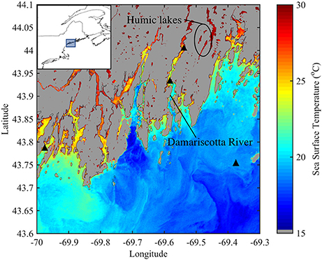
Figure 1. Sea surface temperature on the coast of Maine, USA, on July 14, 2013 from Landsat 8 infrared data. Triangles indicate locations of validation buoys. Freshwater lakes used for the atmospheric correction are circled at ~44′N, −69.5′E.

Processing of Sea Surface Temperature

All applicable raw data from Landsat 8 were downloaded from the USGS Earth Explorer website from the period 2013 to 2016 (USGS, 2016). To calculate SST, we used brightness temperature values from Landsat 8's Thermal Infrared Sensor (TIRS) Band 10. There are stray light issues associated with the two TIRS bands (Band 10 and Band 11) due to the curvature of the optical lens (Montanaro et al., 2014). Of these two bands, we chose to use thermal Band 10 because it has lesser issues of the two (see Discussion Section). Each image was processed in the NASA SeaDAS platform up to level 2 to retrieve latitude and longitude arrays, a geo-registered image, and the associated land/cloud mask (georeferencing is maintained, as it is provided from USGS).

Regressions between coincident, atmospherically corrected NOAA AVHRR satellite derived SST and that derived from Landsat 8's brightness temperature were used to create an SST product from each Landsat 8 image (similar to Thomas et al., 2002). This regression process, de-facto, acts as the atmospheric correction for the Landsat SST product assuming that (1) the atmosphere does not change in the time interval between AVHRR and Landsat data acquisition and (2) the atmosphere is homogenous across the Landsat scene. Example results from this procedure are displayed on Figure 1 above. Of the four to eight AVHRR images captured on the same day as each Landsat 8 overpass, we subjectively chose the image with the least amount of cloud cover, best geolocation, and most realistic SST patterns, for the regression (see Section A in Supplementary Material for detailed description). The data for the regression were selected from cloud free and offshore areas to accommodate the lower AVHRR resolution (1 km vs. Landsat 8 100 m resolution). The best results were achieved using cloud free areas with a high dynamic range in SST. The resulting regression equation between the signal of Landsat's Band 10 and the AVHRR-based SST was then applied to the full resolution Landsat 8 image.

On average, there are approximately four AVHRR images per day. Due to changing cloud cover and orbit configuration between available AVHRR images, it was sometimes necessary to use an image more distant in time (but less cloudy) from the Landsat 8 overpass, despite a temporally more proximate one being available. However, because Gulf of Maine SST patterns change relatively slowly (<0.4°C over 12 h at buoy 44005, www.neracoos.org), we consider this an acceptable tradeoff to maximize the number of quality AVHRR pixels that were used in the regression. The mean offset time between the Landsat 8 and AVHRR overpasses was 6.8 h, with a minimum of 2.3 h, a maximum of 30.2 h, and a standard deviation of 5.8 h. The entire area of spatial overlap between AVHRR ocean pixels and Landsat 8 ocean pixels is used for most scenes. Landsat 8 images were subsampled to every 10th pixel in both x and y dimensions to reduce the data volume for the regressions. Depending on the distribution of clouds, the regression area was restricted to areas without cloud contamination (or poorly masked clouds) in some instances. Cloud and land were dilated by two pixels in the AVHRR image to reduce occurrences of cloud ringing artifacts and nearshore land contamination. The regression process was iterative. After each iteration, all Landsat 8 and coincident AVHRR pixels that were >1 standard deviation from the linear best fit line of the relationship were removed and the regression was re-calculated with the remaining data. The iteration process was repeated until the Pearson correlation coefficient for the two datasets stabilized or started to worsen (which is due to uncertainties in the approach). The final regression equation was then applied to each Landsat 8 B10 pixel to obtain a Landsat SST image.

Ocean Color

Ocean color multispectral data, which responds to the effects of oceanic particles and dissolved matter, are measured from space by the Operational Land Imager (OLI) radiometer on board Landsat 8. The radiance measured includes contributions from the target (the surface water column), the air-water interface, and the background (particles and gases from nearby pixels and particles in the atmosphere) (Mobley et al., 2016). To obtain information on the oceanic constituents, the atmospheric contribution to the signal needs to be removed (a process known as “atmospheric correction,” see below). From the corrected water-leaving radiance, we computed the reflectance (denoted as R_rs) from which the products of turbidity and Chl a are derived.

Atmospheric Correction for R_rs

Given the low turbidity in our area of investigation (see Section Retrieval of Turbidity below), we chose to use a combination of the Near Infrared (NIR) and Short Wave Infrared (SWIR) channels for atmospheric correction in SeaDAS. The NIR was important to use because of its higher signal/noise ratio (NIR band had a ratio of 67 in low turbidity waters, while SWIR bands had ratios of 9 and 10), and the SWIR was important because it has the strongest absorption for water which helps differentiate in-water sediments from atmospheric aerosol particles (Franz et al., 2015; Pahlevan et al., 2017). Applying this atmospheric correction over a scene resulted in a per-pixel correction, each with its own angstrom coefficient. The angstrom coefficient is the exponent of a power-law fit to the spectral aerosol optical thickness. We adjusted this coefficient because the automatic per-pixel retrievals provided by SeaDAS resulted in negative reflectance values at several freshwater bodies that were used as black body targets for our atmospheric correction scheme. These lakes should have near-zero or positive retrievals at the 443 nm band. The primary reason for adjusting the angstrom coefficient is that the aerosol models used for processing data from satellites such as SeaWiFs and MODIS (Ahmad et al., 2010), do not represent the aerosol conditions for our study area, the coast of Maine (Pahlevan et al., 2017). We then chose a single angstrom coefficient per scene (from within the distribution of inverted angstrom values), by requiring that the minimal value of R_rs(443) in a scene, measured in a very humic lake, be zero. Most freshwater lakes on the coast of Maine are humic and have high levels of chromophoric dissolved organic matter, CDOM, which gives them a brown hue and attenuates light quickly (Rasmussen et al., 1989; Roesler and Culbertson, 2016) and are not turbid. Several freshwater lakes with high CDOM within our study region (Muddy Pond, Biscay Pond, and Damariscotta Pond circled in Figure 1) were selected as suitable reference targets to correct the entire Landsat 8 scene. In each individual satellite image, the darkest lake (where R_rs(443) is near zero) was used to determine the angstrom coefficient. Analysis of a sample of water from one of these lakes verified that the expected R_rs(443) is zero within the uncertainty of the satellite retrieval (Table B1 in Supplementary Material). We subsequently applied the retrieved angstrom in SeaDAS to the entire scene to recalculate R_rs at every wavelength. Resulting R_rs values were then used to compute turbidity and Chl a.

Retrieval of Turbidity

Turbidity, T, [note that 1 mg l⁻¹ of suspended particulate matter, SPM, is similar, within the range of values found in our study area, to a turbidity of 1 NTU (Pfannkuche and Schmidt, 2003)], was calculated over the entire satellite scene using atmospherically corrected R_rs(655) following Nechad et al. (2010):

$\begin{array}{ll}\mathrm{\text{T}}={\mathrm{\text{A}}}^{\rho }\frac{{\rho }_{\mathrm{\text{w}}}}{1-{\rho }_{\mathrm{\text{w}}}/{\mathrm{\text{C}}}^{\rho }}\left[\mathrm{\text{g}}{\mathrm{\text{m}}}^{-3}\right]& (1)\end{array}$

where ρ_w = R_rs(655)*π is the atmospherically corrected and derived water leaving reflectance, A^ρ = 289.1 and C^ρ = 16.86 (Nechad et al., 2010).

Retrieval of Chlorophyll- a

Chl a was calculated using the OC3 algorithm (O'Reilly et al., 1998) from the NASA Ocean Biology Processing Group, using the above-calculated R_rs:

$\begin{array}{ll}{log}_{10}(\mathrm{\text{Chl }}a)={\mathrm{\text{a}}}_0+{\displaystyle \sum _{\mathrm{\text{i}}=1}^4}{\mathrm{\text{a}}}_{\mathrm{\text{i}}}{log}_{10}{\left(\frac{{\mathrm{\text{R}}}_{\mathrm{\text{rs}}}\left({\lambda }_{\mathrm{\text{blue}}}\right)}{{\mathrm{\text{R}}}_{\mathrm{\text{rs}}}\left({\lambda }_{\mathrm{\text{green}}}\right)}\right)}^{\mathrm{\text{i}}}& (2)\end{array}$

where a₀ and a_i are sensor specific coefficients, and R_rs(λ_blue) and R_rs(λ_green) are the greatest of values from 443 > 483 and 555 nm, respectively, on the OLI sensor aboard Landsat 8 (NASA, 2016)¹. (Note: SeaDAS applies coefficients to convert broad band Landsat 8-based R_rs to 11 nm narrow bands for which this equation was developed).

Validation with In situ Data

Validation was carried out for SST, turbidity, and Chl a, using data from water samples and three oceanographic buoy observing systems. Historical data was downloaded from the NERACOOS (Northeastern Regional Association of Coastal Ocean Observing Systems) buoys E01 and I01 operated by the University of Maine in the Gulf of Maine, a Land/Ocean Biogeochemical Observatory (LOBO) buoy operated by Bowdoin College in Harpswell Sound, and two LOBO buoys at the University of Maine's Darling Marine Center in the Damariscotta River (Figure 1. Note: NERACOOS Buoy I01 is outside the map). The LOBO buoys were equipped with sensors that remain at a depth of 1.5 m and maintained and cleaned to prevent biofouling approximately every 2 weeks. Temperature data were collected from all three observing systems and compared to Landsat 8 SST. A total of 52 matchups were identified originating from 31 clear overpasses from 2013 to 2016.

In situ turbidity measurements were used to validate satellite-derived turbidity during eight overpasses in 2015 and 2016. Data were collected from the LOBO buoys in the Damariscotta River, and were measured by a WETLabs WQM sensor capable of measuring turbidity from 0 to 25 NTU (using a backscattering sensor measuring light scattered in the back direction at a 20 nm bandwidth around 700 nm). This sensor was vicariously calibrated against a Hach turbidity sensor (which conform to the ISO 7027:1999 turbidity standard). The buoy data were calibrated using a regression between Hach turbidity samples and the LOBO turbidity using a factor of 1.58 (Table B2 in Supplementary Material).

In situ Chl a was used to validate satellite-derived Chl a during the same eight overpasses in 2015 and 2016. In situ Chl a data were measured by the Damariscotta River LOBO buoys' WETLabs fluorescent sensor capable of measuring Chl a concentrations from 0 to 50 μgl⁻¹. The buoy data were calibrated using a regression between extracted Chl a samples and the LOBO Chl a using a factor of 1.71. Water samples were collected in triplicate, at the surface, and in opaque bottles within 30 min of each overpass and filtered for extraction on a Turner 10 AU fluorometer per standard protocol (Holm-Hansen and Riemann, 1978). Statistics were calculated for regressions between the in situ and satellite-derived data: Root mean square difference, RMSD, root mean square relative difference, RRMSD, and coefficient of determination, r² (see Figures 2–4 below).

FIGURE 2

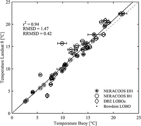
Figure 2. Type II linear regression (black line) between Landsat 8-derived SST and SST measured by sensors on oceanographic buoys. Different symbols represent measurements by the three different observing systems. Vertical error bars are the standard deviation of a 5 × 5 pixel box. Horizontal error bars are the standard deviation of daily temperature at each buoy. Dashed gray line is 1:1.

Satellite Imagery for Oyster Suitability Index

An Oyster Growth Suitability Index (OSI) was designed using the satellite-derived SST, turbidity, and Chl a. A weighting and indexing procedure of these three physical parameters described ideal, moderate, and poor conditions for growing market sized oysters in surface culture. The criteria for the index were chosen based on published studies of environmental effects on oyster growth, recognizing that the concentration of organic detritus, known to be an important component of oyster diet, was not available. Temperature is the most important variable for oyster growth, especially in the cold waters of coastal Maine as it controls the filtration rate of oysters [and therefore given an importance weight factor of 80% in our OSI; (Loosanoff, 1958; Hoffmann et al., 1992; Ehrich and Harris, 2015)]. Oyster clearance of algae is a positive function of algae concentration, as large amounts of pseudofeces are produced at high algal concentrations. Because of this, we weighted Chl a at 15%, with poor conditions as <1 or >10 μg Chl l⁻¹, moderate conditions as 1 to 3 μg Chl l⁻¹, and ideal conditions as 3 to 10 μg Chl l⁻¹ (Epifanio and Ewart, 1977; Hawkins et al., 2013b). Turbidity, an index of suspended particulate matter, has a negative effect on oyster feeding when at high concentrations, by diluting algal cells with largely inorganic matter. Haven and Morales-Alamo (1966) observed large amounts of pseudofeces production by Eastern oysters at concentrations of suspended particulate matter above 10 mg l⁻¹. Thus, we gave turbidity a weight of 5% and designated poor conditions as >10 mg l⁻¹, moderate conditions between 8 and 10 mg l⁻¹ and ideal conditions <8 mg l⁻¹. Hoffmann et al. (1992) also modeled oyster filtration as a positive function of water temperature and a negative function of high suspended loads.

These weights are subjective and were chosen as a starting point for an OSI. They could be refined in the future (Gong et al., 2012), based on sensitivity analysis of the relative importance of these factors measured simultaneously with growth measurements in situ. The resulting OSI is the sum of the weighted conditions on a scale from 0 to 1, where pixels with a value of 1 represent waters where an oyster is likely to grow to market size within 2 years:

$\begin{array}{ll}\mathrm{\text{OSI}}={\displaystyle \sum _{\mathrm{\text{i}}=1}^{\mathrm{\text{n}}}}\mathrm{\text{S}}{\mathrm{\text{I}}}_{\mathrm{\text{i}}}\times {\mathrm{\text{w}}}_{\mathrm{\text{i}}}& (3)\end{array}$

where SI_i is the value of the environmental variable i, w_i is the weight of the variable i, and n is the number of environmental variables (three in our case). At any location where one of the three indices reported poor conditions, the OSI was set to zero. We combined images from each year during the same month to create a monthly averaged index.

Results

Validation with In situ Data

The Landsat 8 SST retrievals correlated well with in situ temperatures (RMSD is 0.82°C, RRMSD is 4%, r² = 0.94) with, on average, 1°C higher SST values than those measured by the buoy sensors, especially in warmer waters (Figure 2). However, variability of the buoy measurements is larger at higher temperatures when horizontal gradients in temperature were also larger.

The Landsat 8 turbidity estimates correlated well with in situ turbidities (RMSD 0.49 NTU, RRMSD 3%, max absolute deviation is 0.96 and maximal relative deviation is 15%, r² = 0.88), with an uncertainty of 0.5 NTU, on average (Figures 3A,B). Uncertainties are larger at higher turbidities for both the buoy and the satellite algorithm.

FIGURE 3

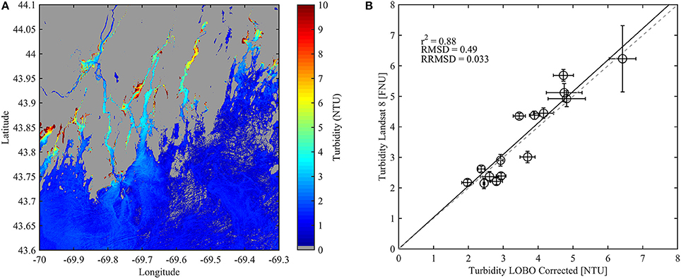
Figure 3. (A) Landsat 8-derived turbidity along mid-coast Maine on July 14, 2013. (B) Type II linear regression (black line) between Landsat 8-derived turbidity and turbidity measured by LOBO buoys. Vertical error bars are the standard deviation of a 5 × 5 pixel box centered at the in situ measurement. Horizontal error bars are the standard deviation of turbidity for 4 h at each buoy. Dashed gray line is 1:1.

Landsat 8 based Chl a did not correlate well with in situ Chl a (RMSD is 1.75 μg Chl l⁻¹, RRMSD is 110%, max absolute deviation is 3.14 μg Chl l⁻¹, max relative deviation is 156%, r² = 0.31). Below 5 μg Chl l⁻¹, the OC3 algorithm produced higher Chl a values than those measured by the buoy sensors (Figures 4A,B). Above 5 μg Chl l⁻¹, the buoy measurements were higher than the satellite-derived Chl a. Uncertainties are larger at higher Chl a for the buoys and the satellite algorithm. Out of the three parameters derived from Landsat 8, this algorithm has the highest relative deviation of 156%, with an average relative difference of 110%, which is significantly worse than the average relative difference of 30% for chlorophyll algorithms in the open ocean (but see Discussion).

FIGURE 4

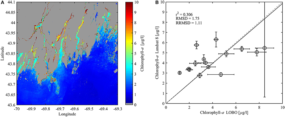
Figure 4. (A) Landsat 8-derived chlorophyll-a along mid-coast Maine on July 14, 2013. (B) Type II linear regression (black line) between Landsat 8 derived chlorophyll-a and chlorophyll-a measured by LOBO buoys. Vertical error bars are the standard deviation of a 5 × 5 pixel box centered at the in situ measurement. Horizontal error bars are the standard deviation of chlorophyll-a for 4 h at each buoy. Buoy chlorophyll-a was calibrated with chlorophyll extraction samples. Dashed gray line is 1:1.

Satellite Imagery for Oyster Growth Conditions

Monthly maps of Oyster Suitability Index (Figure 5) were created using averaged monthly satellite images (Section B in Supplementary Material). Most existing oyster aquaculture areas (indicated by red stars on Figure 5) fall within the highest suitability index during the month of July. Suitability maps for August and September exhibit a similar pattern of ideal, moderate, and poor growing areas as the map for July (Figure 5), but, in general, with slightly lower values due to colder temperatures (average monthly temperatures were highest during July). The Oyster Suitability Index map provides two important findings: (1) it is consistent in its finding that the Damariscotta River as a suitable place to grow oysters in aquaculture and therefore an important test and verification site for using remote sensing tools, and (2) it maps many new locations along the coast that host similar conditions (Table B2 in Supplementary Material).

FIGURE 5

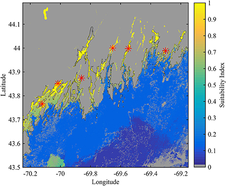
Figure 5. Oyster suitability map based on Landsat 8-derived SST, turbidity, and chlorophyll-a. Map is an average of all images in the month of July. Yellow areas indicate ideal conditions, green areas indicate moderate conditions, and blue areas indicate poor conditions. Red stars indicate existing oyster farms. Index criteria is given in Section B in Supplementary Material.

Discussion

Satellite Imagery

The correspondence between the Landsat 8 satellite-derived products and in situ measurements demonstrates the capability of generating SST, turbidity, and Chl a maps along the jagged coast of Maine. While these data show encouraging results, there are several factors from our study that could improve the present algorithms. Stray light issues arise if the temperature from an object outside of the field of view of the imager affects the pixel within the field of view. Fortunately, most water along the coast of Maine is vigorously tidally mixed (~3 m tidal range), and thus data from the center of channels can be used to infer SST throughout those channels (Thornton and Mayer, 2015). Within the estuaries, however, a TIRS pixel (which is three times as wide as an OLI pixel) next to land may be incorrectly colder (if the land is colder) or warmer (if the land is warmer). However, our match-ups with temperature and turbidity products suggest adjacency and stray light have not degraded the data significantly, and differences are likely due to noise as opposed to systematic bias.

Limitations in Validation Process

Validation of Landsat 8 products with in situ measurements is necessary to assess the accuracy of the algorithms for retrieving bio-physical products. Some of the discrepancy in matchups between in situ data and satellite-derived products can be explained, while others require further investigation. One reason that Landsat 8 SST values may be higher than most buoy measurements (Figure 2) is because the SST estimates come from radiation emitted from the top few micrometers of the sea surface, while the buoy sensors are located about 1.5 m below the surface. In the daytime images, the subsurface water is likely cooler than the surface skin due to physical and environmental factors (Donlon et al., 2002; Ward, 2006; Padula et al., 2010). Despite this bias, the Landsat 8 SST (derived by regressing with atmospherically-corrected AVHRR SST) performed well along the coast of Maine and our results suggest that our approach could be used as a tool for measuring SST where high spatial resolution is desired.

A vigorous semi-diurnal tide characterizes the Damariscotta River and delivers shelf water into the upper reaches of the estuary. The tidal cycle was evident in the daily turbidity signal (not shown) from the LOBO buoys: at low tide, there are elevated levels of turbidity whereas at high tide there is less turbidity (due to the increase in turbidity from the mouth to the end of the estuary). The horizontal error bars in Figure 3 represent the variability during a 4-h period around each satellite overpass time, and highlight the importance of simultaneous sampling for in situ—satellite matchups. The turbidity algorithm performs well within our uncertainties in this context.

Landsat 8-derived Chl a often differs significantly from the LOBO buoy measurements. We note that there are significant uncertainties associated with both measurement techniques (Cullen, 2008). Landsat 8-derived Chl a is retrieved from R_rs using an algorithm calibrated in the open ocean, whereas the LOBO buoys measure Chl a fluorescence which is regressed against chlorophyll measured on water samples. Estimating Chl a from fluorescence is the most common way to measure Chl a but is affected by several processes that contribute to uncertainty. These include changes in fluorescence yield due to variability in the algal taxonomy, nutrient stress, and photo-acclimation, to name a few (Cullen, 1982). In addition, concentrations of phytoplankton have been observed in the Damariscotta River to vary on time scales of hours (Thompson and Perry, 2006) potentially making mismatches in time problematic.

Non-photochemical quenching (NPQ; when phytoplankton decrease their fluorescence at a maximum light harvesting level, e.g., Cullen, 1982) contributes to variability. However, we find nighttime measurements to be comparable to daytime measurements (Figure B1 Supplementary Material) for the Damariscotta River. Therefore, the offset in Chl a is likely not due to errors induced by NPQ. Another potential error is associated with the OC3 algorithm, which estimates Chl a as a ratio of R_rs in the blue and green channels. The blue channel is especially influenced by colored dissolved organic material (CDOM). Independent changes of CDOM will affect the OC3 chlorophyll estimate (Siegel et al., 2005). Along the coast of Maine, where there are coastal forests and marshes, CDOM is in high concentration and variable (Roesler and Culbertson, 2016). In coastal areas and estuaries rich in CDOM it is likely that absorption by dissolved organic matter would bias the OC3 algorithm. It is likely that a local algorithm that takes local CDOM concentration into account, could improve Chl a retrievals from Landsat 8.

Oyster Suitability Index

The OSI provided in this paper is intended to supplement other tools that determine optimal oyster growing areas. The satellite images, due to their low temporal resolution, provide a climatological monthly average of coastal temperature, which does not resolve the day degree input necessary in models for temperature-dependent shellfish growth. In addition, other important environmental factors such as salinity, water depth, bottom type, and water velocity (necessary for oyster growing), are not considered (Theuerkauf and Lipcius, 2016). Organic detritus is known to be an important component of bivalve diets (Dame and Patten, 1981; Bayne et al., 1993; Barillé et al., 1997), but currently cannot be measured using satellite imagery. It is conceivable that detritus could be related to the ratio of turbidity and Chl a, after light acclimation has been accounted for. Our index therefore provides guidance on suitable water quality conducive to rapid growth, but not sufficient information to model site specific production capacity for suspended or bottom culture.

Although, satellite thermal data is only sensitive to the temperature of the top few micrometers of water, and ocean color is sensitive only to one optical depth (which varies, but on the Maine coast is usually the top 1 or 2 m), these data are relevant to the whole water column if the water column is often vertically well-mixed. Indeed, many estuaries on the Maine coast are well-mixed (e.g., the Sheepscot and Medomak Rivers, Mayer, 1996; Thornton and Mayer, 2015), which makes it relevant for our OSI (Table B2 in Supplementary Material). Finally, local knowledge is invaluable for the expansion of an existing industry on the coast of Maine, and stakeholder input is essential for improving such an index with local information such as site accessibility, town ordinances, etc.

Future Work

Continued sampling during the spring and summer of 2017 will provide a more complete dataset for optimizing Landsat-derived products in Maine. A local algorithm for Landsat 8-derived Chl a along the coast of Maine could be constructed with additional in situ samples collected during satellite overpasses. There are several approaches to tune a local algorithm. An empirical approach, such as the OC3 algorithm, uses a relationship between in situ measurements and ratios of the satellite sensor bands. A second method involves using a generalized inherent optical properties inversion (GIOP, Werdell et al., 2013). This method solves for Chl a, SPM, and CDOM using known spectral shapes of optical properties (for phytoplankton and non-algal absorption and backscattering by particles) and known values of absorbance and backscattering of water (which are weak functions of salinity and temperature). Databases of collection sites located in the Damariscotta River and Harpswell Sound could tune the shapes of IOPs for the GIOP algorithm and provide an estimate of Chl a in these two estuaries. Furthermore, in situ samples from various locations along the coast will validate the local algorithm so that its use can be expanded from the Damariscotta River to other places along the coast.

Obtaining more parameters from Landsat 8, such as colored dissolved organic matter (CDOM), would provide additional information to growers and ecosystem managers. Franz et al. (2015) and Slonecker et al. (2015) describe the potential of using Landsat 8 for remote sensing of CDOM in conjunction with in situ measurements. A reliable CDOM product would also improve the algorithm for Chl a, as the presence of CDOM often contributes to an overestimation of Chl a. Furthermore, high levels of CDOM are correlated with low salinity in estuaries (Carder et al., 1989; D'Sa et al., 2002; Mayer, pers. commun.). CDOM would therefore be helpful to identify areas with significant freshwater influx because these often bring concentrations of bacteria that negatively affect clamming and other fisheries (Shumway et al., 1988; Kleindinst et al., 2014).

Validation of our OSI is provided by the fact that current farms are all located where the OSI is high. Further validation and refinement with direct measurements of oyster growth, will likely improve on this OSI. Note: OSI does not include information about site closures, bottom depth, or residential restrictions. Future work should include this information for a more comprehensive index.

Conclusion

A satellite-derived Oyster Suitability Index can act as a powerful tool for oyster aquaculture site selection and the expansion of the shellfish farming industry. It shows that suitable biophysical conditions for oyster growth exist in many areas of the Maine coast. Suitability indices for other bivalve species, such as mussels, scallops, and finfish along the coast, or other applications requiring high spatial resolution, can be developed based on the algorithms presented here.

Our results show that Landsat 8-derived data are useful for retrieving SST, turbidity, and Chl a in coastal waters of Maine, USA, and can be applied to other narrow estuaries around the world. The novelty of using Landsat 8 in this context offers a unique opportunity to map and monitor coastal waters at an unprecedented spatial resolution. Inclusion of data from other satellites with complimentary sensor suites such as Sentinel 2A, and the recently launched Sentinel 2B, could improve both the spatial and temporal coverage of coastal waters, as they will provide five-day or better coverage and more visible bands to derive products with (unfortunately, Sentinel 2A and B do not have thermal bands), and be used to study oyster growing facilities (Gernez et al., 2017). SST data from Landsat 8 is especially useful for aquaculture site prospecting. We recommend adding thermal bands to high resolution instruments on future missions. Future work improving biogeochemical local algorithms, refining the atmospheric correction, and adding other parameters such as CDOM, will further advance the use of high resolution remote-sensing for coastal applications.

Author Contributions

EB, AT, CN, and DB provided contributions for the design of the work. JS, RW, and EB contributed to data acquisition and analysis. JS was responsible for conducting field work and buoy maintenance in the Damariscotta River. JS, RW, EB, and CN were responsible for drafting the work, and all authors were responsible for revisions and final approval.

Funding

This project is supported by National Sea Grant award E-14-EA-2, the National Science Foundation award #11A-1355457 to Maine EPSCoR at the University of Maine, the NASA Ocean Biology and Biogeochemistry program Grant #NNX14AP66G, and the NASA EPSCoR program to Maine Space Grant.

Conflict of Interest Statement

The authors declare that the research was conducted in the absence of any commercial or financial relationships that could be construed as a potential conflict of interest.

Acknowledgments

Thank you to Catherine Coupland, Nicolas DelPrete, Tiega Martin, Chris Rigaud, Matthew Grey, and Robbie Downs for their assistance maintaining the LOBO buoys at the Darling Marine Center. Thank you to Nils Haëntjens for assistance with data processing. Thank you to Jocelyn Runnebaum, Kevin Staples, and Nils Haëntjens for the helpful edits. Thank you to the SEANET project at University of Maine for providing LOBO buoy data and travel support. We thank our two reviewers for their input which resulted in a better manuscript.

Supplementary Material

The Supplementary Material for this article can be found online at: https://www.frontiersin.org/article/10.3389/fmars.2017.00190/full#supplementary-material

Footnotes

1. ^NASA (2016). Available online at: https://oceancolor.gsfc.nasa.gov/atbd/chlor_a/

References

Aguilar Manjarrez, J., and Crespi, V. (2013). Aquaculture Newsletter 55, September 2016. Rome: FAO.

Ahmad, Z., Franz, B. A., McClain, C. R., Kwiatkowska, E. J., Werdell, J., Shettle, E. P., et al. (2010). New aerosol models for the retrieval of aerosol optical thickness and normalized water-leaving radiances from the SeaWiFS and MODIS sensors over coastal regions and open oceans. Appl. Opt. 49:5545. doi: 10.1364/ao.49.005545

PubMed Abstract | CrossRef Full Text | Google Scholar

Barillé, L., Prou, J., Héral, M., and Razet, D. (1997). Effects of high natural seston concentrations on the feeding, selection, and absorption of the oyster Crassostrea gigas (Thunberg). J. Exp. Mar. Biol. Ecol. 212, 149–172. doi: 10.1016/S0022-0981(96)02756-6

CrossRef Full Text | Google Scholar

Barnes, T. K., Volety, A. K., Chartier, K., Mazzotti, F. J., and Pearlstine, L. (2007). A habitat suitability index model for the eastern oyster (Crassostrea virginica), a tool for restoration of the Caloosahatchee Estuary, Florida. J. Shellfish Res. 26, 949–959. doi: 10.2983/0730-8000(2007)26[949:AHSIMF]2.0.CO;2

CrossRef Full Text | Google Scholar

Bayne, B. L., Iglesias, J. I. P., Hawkins, A. J. S., Navarro, E., Heral, M., and Deslous-Paoli, J. M. (1993). Feeding behaviour of the mussel, Mytilus edulis: responses to variations in quantity and organic content of the seston. J. Mar. Biol. Assoc. United Kingdom 73, 813–829. doi: 10.1017/S0025315400034743

CrossRef Full Text | Google Scholar

Cake, E. W. Jr. (1983). Habitat Suitability Index Models: Gulf of Mexico American Oyster (No. 82/10.57). U.S. Fish and Wildlife Service.

Google Scholar

Carder, K. L., Steward, R. G., Harvey, G. R., and Ortner, P. B. (1989). Marine humic and fulvic acids: their effects on remote sensing of ocean chlorophyll. Limnol. Oceanogr. 34, 68–81. doi: 10.4319/lo.1989.34.1.0068

CrossRef Full Text | Google Scholar

Carrasco, M. F., and Barón, P. J. (2010). Analysis of the potential geographic range of the Pacific oyster Crassostrea gigas (Thunberg, 1793) based on surface seawater temperature satellite data and climate charts: the coast of South America as a study case. Biol. Invasions 12, 2597–2607. doi: 10.1007/s10530-009-9668-0

CrossRef Full Text | Google Scholar

Congleton, W. R., Pearce, B. R., Parker, M. R., and Beal, B. F. (1999). Mariculture siting: a GIS description of intertidal areas. Ecol. Model. 116, 63–75. doi: 10.1016/S0304-3800(98)00158-6

CrossRef Full Text | Google Scholar

Cullen, J. J. (1982). The deep chlorophyll maximum: comparing vertical profiles of chlorophyll a. Can. J. Fish. Aqu. Sci. 39, 791–803. doi: 10.1139/f82-108

CrossRef Full Text | Google Scholar

Cullen, J. J. (2008). “Observation and prediction of harmful algal blooms,” in Real-Time Coastal Observing Systems for Ecosystem Dynamics and Harmful Algal Blooms, eds M. Babin, C. S. Roesler, and J. J. Cullen (Paris: UNESCO).

Dame, R. F., and Patten, B. C. (1981). Analysis of energy flows in an intertidal oyster reef. Mar. Ecol. Prog. Ser. 5, 115–124. doi: 10.3354/meps005115

CrossRef Full Text | Google Scholar

Dogliotti, A. I., Ruddick, K. G., Nechad, B., Doxaran, D., and Knaeps, E. (2015). A single algorithm to retrieve turbidity from remotely-sensed data in all coastal and estuarine waters. Remote Sens. Environ. 156, 157–168. doi: 10.1016/j.rse.2014.09.020

CrossRef Full Text | Google Scholar

Donlon, C. J., Minnett, P. J., Gentemann, C., Nightingale, T. J., Barton, I. J., Ward, B., et al. (2002). Toward improved validation of satellite sea surface skin temperature measurements for climate research. J. Climate 15, 353–369. doi: 10.1175/1520-0442(2002)015<0353:TIVOSS>2.0.CO;2

CrossRef Full Text | Google Scholar

D'Sa, E., Hu, C., Muller-Karger, F., and Carder, K. (2002). Estimation of colored dissolved organic matter and salinity fields in case 2 waters using SeaWiFS: examples from Florida Bay and Florida Shelf. J. Earth Syst. Sci. 111, 197–207. doi: 10.1007/BF02701966

CrossRef Full Text

Ehrich, M. K., and Harris, L. A. (2015). A review of existing eastern oyster filtration rate models. Ecol. Model. 297, 201–212. doi: 10.1016/j.ecolmodel.2014.11.023

CrossRef Full Text | Google Scholar

Epifanio, C. E., and Ewart, J. (1977). Maximum ration of four algal diets for the oyster Crassostrea virginica Gmelin. Aquaculture 11, 13–29. doi: 10.4319/lo.1966.11.4.0487

CrossRef Full Text | Google Scholar

Franz, B. A., Bailey, S. W., Kuring, N., and Werdell, P. J. (2015). Ocean color measurements with the operational land imager on landsat-8: implementation and evaluation in SeaDAS. J. Appl. Remote Sens. 9:96070. doi: 10.1117/1.JRS.9.096070

CrossRef Full Text | Google Scholar

Gernez, P., Doxaran, D., and Barille, L. (2017). Shellfish Aquaculture from Space: potential of Sentinel2 to monitor tide-driven changes in turbidity, chlorophyll concentrations and oyster physiological response at the scale of an oyster farm. Front. Mar. Sci. 4:137. doi: 10.3389/fmars.2017.00137

CrossRef Full Text | Google Scholar

Gernez, P., Lerouxel, A., Mazeran, C., Lucas, A., and Barill, L. (2014). Remote sensing of suspended particulate matter in turbid oyster-farming ecosystems. J. Geophys. Res. 119, 7277–7294. doi: 10.1002/2014jc010055

CrossRef Full Text | Google Scholar

Gong, C., Chen, X., Gao, F., and Chen, Y. (2012). Importance of weighting for multi-variable habitat suitability index model: a case study of winter-spring cohort of Ommastrephes bartramii in the Northwestern Pacific Ocean. J. Ocean Univers. China 11, 241–248. doi: 10.1007/s11802-012-1898-6

CrossRef Full Text | Google Scholar

Haven, D. S., and Morales-Alamo, R. (1966). Aspects of biodeposition by oysters and other invertebrate filter feeders. Limnol. Oceanogr. 11, 487–498. doi: 10.4319/lo.1966.11.4.0487

CrossRef Full Text | Google Scholar

Hawkins, A. J. S., Pascoe, P. L., Parry, H., Brinsley, M., Black, K. D., McGonigle, C., et al. (2013a). Shellsim: a generic model of growth and environmental effects validated across contrasting habitats in bivalve shellfish. J. Shellfish Res. 32, 237–253. doi: 10.2983/035.032.0201

CrossRef Full Text | Google Scholar

Hawkins, A. J. S., Pascoe, P. L., Parry, H., Brinsley, M., Cacciatore, F., Black, K. D., et al. (2013b). Comparative feeding on chlorophyll-rich versus remaining organic matter in bivalve shellfish. J. Shellfish Res. 32, 883–897. doi: 10.2983/035.032.0332

CrossRef Full Text | Google Scholar

Hoffmann, E. E., Powell, E. N., Klinck, J. M., and Wilson, E. A. (1992). Modeling oyster populations III. Critical feeding periods, growth. J. Shellfish Res. 11, 399–416.

Google Scholar

Holm-Hansen, O., and Riemann, B. (1978). Chlorophyll a determination: improvements in methodology. Oikos 30, 438–447. doi: 10.2307/3543338

CrossRef Full Text | Google Scholar

Kleindinst, J. L., Anderson, D. M., McGillicuddy, D. J., Stumpf, R. P., Fisher, K. M., Couture, D. A., et al. (2014). Categorizing the severity of paralytic shellfish poisoning outbreaks in the Gulf of Maine for forecasting and management. Deep Sea Res. II 103, 277–287. doi: 10.1016/j.dsr2.2013.03.027

PubMed Abstract | CrossRef Full Text | Google Scholar

Loosanoff, V. L. (1958). Some aspects of behavior of oysters at different temperatures. Biol. Bull. 114, 57–70. doi: 10.2307/1538965

CrossRef Full Text | Google Scholar

Mayer, L. M. (1996). The Kennebec, Sheepscot and Damariscotta River Estuaries: Seasonal Oceanographic Data. University of Maine at Orono and University of Maine/University of New Hampshire Sea Grant College, Program. Orono, ME: Dept. of Oceanography, University of Maine.

McAlice, B. J. (1977). A Preliminary Oceanographic Survey of Damariscotta River Estuary, Lincoln County, Maine. Washington: US National Oceanic and Atmospheric Administration.

Mobley, C. D., Werdell, J., Franz, B., Ahmad, Z., and Bailey, S. (2016). Atmospheric Correction for Satellite Ocean Color Radiometry A Tutorial and Documentation NASA Ocean Biology Processing Group.

Montanaro, M., Gerace, A., Lunsford, A., and Reuter, D. (2014). Stray light artifacts in imagery from the landsat 8 thermal infrared sensor. Remote Sens. 6, 10435–10456. doi: 10.3390/rs61110435

CrossRef Full Text | Google Scholar

Nechad, B., Ruddick, K. G., and Park, Y. (2010). Calibration and validation of a generic multisensor algorithm for mapping of total suspended matter in turbid waters. Remote Sens. Environ. 114, 854–866. doi: 10.1016/j.rse.2009.11.022

CrossRef Full Text | Google Scholar

Newell, C. R., Hawkins, A. J. S., Morris, K., Richardson, J., Davis, C., and Getchis, T. (2013). ShellGIS: a dynamic tool for shellfish farm site selection. World Aquacult. 44, 50–53. Available online at: http://www.was.org/magazine/Contents.aspx?Id=47

Google Scholar

Newell, C. R., Shumway, S., Cucci, T. L., and Selvin, R. (1989). The effects of natural seston particle size and type on feeding rates, feeding selectivity and food resource availability for the mussel Mytilus edulis Linnaeus, 1758 at bottom culture sites in Maine. J. Shellfish Res. 8, 187–196.

Newell, R. I. E., and Jordan, S. J. (1983). Preferential ingestion of organic material by the American oyster Crassostrea virginica. Mar. Ecol. Prog. Ser. Oldendorf 13, 47–53. doi: 10.3354/meps013047

CrossRef Full Text | Google Scholar

O'Reilly, J. E., Maritorena, S., Mitchell, B. G., Siegel, D. A., Carder, K. L., Garver, S. A., et al. (1998). Ocean color chlorophyll algorithm for SeaWiFS. J. Geophys. Res. 103, 24937–24953.

Google Scholar

Pahlevan, N., Lee, Z., Wei, J., Schaaf, C. B., Schott, J. R., and Berk, A. (2014). On-orbit radiometric characterization of OLI (Landsat-8) for applications in aquatic remote sensing. Remote Sens. Environ. 154, 272–284. doi: 10.1016/j.rse.2014.08.001

CrossRef Full Text | Google Scholar

Pahlevan, N., Roger, J.-C., and Ahmad, Z. (2017). Revisiting short-wave-infrared (SWIR) bands for atmospheric correction in coastal waters. Opt. Express 25, 6015–6035. doi: 10.1364/OE.25.006015

PubMed Abstract | CrossRef Full Text | Google Scholar

Pérez-Camacho, A., Aguiar, E., Labarta, U., Vinseiro, V., Fernández-Reiriz, M. J., and Álvarez-Salgado, X. A. (2014). Ecosystem-based indicators as a tool for mussel culture management strategies. Ecol. Indic. 45, 538–548. doi: 10.1016/j.ecolind.2014.05.015

CrossRef Full Text | Google Scholar

Pfannkuche, J., and Schmidt, A. (2003). Determination of suspended particulate matter concentration from turbidity measurements: particle size effects and calibration procedures. Hydrol. Process. 17, 1951–1963. doi: 10.1002/hyp.1220

CrossRef Full Text | Google Scholar

Powell, E. N., Hofmann, E. E., Klinck, J. M., and Ray, S. M. (1992). Modeling oyster populations 1. A commentary on filtration rate. Is faster always better? J. Shellfish Res. 1, 387–398.

Google Scholar

Padula, F. P., Schott, J. R., Barsi, J. A., Raqueno, N. G., and Hook, S. J. (2010). Calibration of Landsat 5 thermal infrared channel: updated calibration history and assessment of the errors associated with the methodology. Can. J. Remote Sens. 36, 617–630. doi: 10.5589/m10-084

CrossRef Full Text | Google Scholar

Radiarta, I. N., Saitoh, S. I., and Miyazono, A. (2008). GIS-based multi-criteria evaluation models for identifying suitable sites for Japanese scallop (Mizuhopecten yessoensis) aquaculture in Funka Bay, southwestern Hokkaido, Japan. Aquaculture 284, 127–135. doi: 10.1016/j.aquaculture.2008.07.048

CrossRef Full Text | Google Scholar

Rasmussen, J. B., Godbout, L., and Schallenburg, M. (1989). The humic content of lake water and its relationship to watershed and lake morphometry. Limnol. Oceanogr. 34, 1336–1343. doi: 10.4319/lo.1989.34.7.1336

CrossRef Full Text | Google Scholar

Rheault, R. B., and Rice, M. A. (1996). Food-limited growth and condition index in the eastern oyster, Crassostrea virginica (Gmelin 1791), and the bay scallop, Argopecten irradians irradians (Lamarck 1819). J. Shellfish Res. 15, 271–283.

Roesler, C., and Culbertson, C. (2016). “Lake transparency: a window into decadal variations in dissolved organic carbon concentrations in lakes of Acadia National Park, Maine,” in Aquatic Microbial Ecology and Biogeochemistry: A Dual Perspective, eds P. M. Glibert and T. M. Kana (Springer International Publishing Switzerland), 225–236. doi: 10.1007/978-3-319-30259-1

CrossRef Full Text | Google Scholar

Shumway, S. E., Sherman-Caswell, S., and Hurst, J. (1988). Paralytic shellfish poisoning in Maine: monitoring a monster. J. Shellfish Res. 7, 643–652.

Google Scholar

Siegel, D. A., Maritorena, S., Nelson, N. B., and Behrenfeld, M. J. (2005). Independence and interdependencies among global ocean color properties: reassessing the bio-optical assumption. J. Geophys. Res. C 110, 1–14. doi: 10.1029/2004jc002527

CrossRef Full Text | Google Scholar

Slonecker, E. T., Jones, D. K., and Pellerin, B. A. (2015). The new Landsat 8 potential for remote sensing of colored dissolved organic matter (CDOM). Mar. Pollut. Bull. 107, 518–527. doi: 10.1016/j.marpolbul.2016.02.076

PubMed Abstract | CrossRef Full Text | Google Scholar

Soniat, T. M., and Brody, M. S. (1988). Field validation of a habitat suitability index model for the American oyster. Estuaries Coasts 11, 87–95. doi: 10.2307/1351995

CrossRef Full Text | Google Scholar

Theuerkauf, S. J., and Lipcius, R. N. (2016). Quantitative validation of a habitat suitability index for oyster restoration. Front. Mar. Sci. 3:64. doi: 10.3389/fmars.2016.00064

CrossRef Full Text | Google Scholar

Thomas, A., Byrne, D., and Weatherbee, R. (2002). Coastal sea surface temperature variability from Landsat infrared data. Remote Sens. Environ. 81, 262–272. doi: 10.1016/S0034-4257(02)00004-4

CrossRef Full Text | Google Scholar

Thomas, Y., Mazurié, J., Alunno-Bruscia, M., Bacher, C., Bouget, J. F., Gohin, F., et al. (2011). Modelling spatio-temporal variability of Mytilus edulis (L.) growth by forcing a dynamic energy budget model with satellite-derived environmental data. J. Sea Res. 66, 308–317. doi: 10.1016/j.seares.2011.04.015

CrossRef Full Text | Google Scholar

Thompson, B. P., and Perry, M. J. (2006). Temporal and Spatial Variability of Phytoplankton Biomass in the Damariscotta River Estuary, Maine, U.S.A. Thesis, Department of Marine Sciences.

Thornton, K., and Mayer, L. (2015). Maine Coastal Observing Alliance. Summary Report 2014.

USGS (2016). L8 OLI/TIRS Product. Available online at: https://earthexplorer.usgs.gov

Vanhellemont, Q., and Ruddick, K. (2014). Turbid wakes associated with offshore wind turbines observed with Landsat 8. Remote Sens. Environ. 145, 105–115. doi: 10.1016/j.rse.2014.01.009

CrossRef Full Text | Google Scholar

Wang, H., Hladik, C. M., Huang, W., Milla, K., Edmiston, L., Schalles, J. F., et al. (2010). Detecting the spatial and temporal variability of chlorophyll-a concentration and total suspended solids in Apalachicola Bay, Florida using MODIS imagery. Int. J. Remote Sens. 31, 439–453. doi: 10.1080/01431160902893485

CrossRef Full Text | Google Scholar

Ward, B. (2006). Near-surface ocean temperature. J. Geophys. Res. 111, 1–18. doi: 10.1029/2004jc002689

CrossRef Full Text | Google Scholar

Werdell, P. J., Franz, B. A., Bailey, S. W., Feldman, G. C., Boss, E., Brando, V. E., et al. (2013). Generalized ocean color inversion model for retrieving marine inherent optical properties. Appl. Optics 52, 2019–2037. doi: 10.1364/AO.52.002019

PubMed Abstract | CrossRef Full Text | Google Scholar

Widdows, J., Fieth, P., and Worrall, C. M. (1979). Relationships between seston, available food and feeding activity in the common mussel Mytilus edulis. Mar. Biol. 50, 195–207. doi: 10.1007/bf00394201

CrossRef Full Text | Google Scholar