Estuarine Suspended Sediment Dynamics: Observations Derived from over a Decade of Satellite Data

Introduction

Estuaries are highly dynamic environments. They exist in transitional zones where riverine systems combine with oceanic systems and exhibit characteristics of both, such as floods and droughts as well as tides and waves. Suspended sediments are an integral part of estuarine systems; their flux within estuaries is a result of interplay between freshwater inflow, tidal currents, wind-wave resuspension, commercial fishing, and dredging operations (Ward and Montague, 1996). The relative importance of physical processes influencing the spatial distributions of suspended sediments varies as a function of time and space, morphology, bathymetry, and regional climate, however, the influence of anthropogenic activities is largely unknown (Ward and Montague, 1996; Green and Coco, 2014).

Most US state and federal agencies use a few point measurements within estuarine systems to characterize overall conditions. Typically, suspended sediment concentrations have been quantified by collecting water samples from discrete locations within an estuary and measuring their total suspended solids (TSS) concentrations (Ward and Montague, 1996). For temporal studies, the sampling is repeated at the same station over time, thus providing insight into the processes ongoing in the area (Shideler, 1984). The spatial resolution of this approach, however, is limited by time and expense thus restricting the number of regularly sampled locations. Conditions observed at a single point, however, can be the result of many complex and interrelated processes. Early attempts to bridge this spatial gap in Texas included eight repeated sample collections at 14 locations within 5 h, in Corpus Christi Bay using a helicopter (Shideler, 1984). Shideler's study produced some of the first quasi-synoptic measurements of suspended sediments in this region and documented the dominant spatial patterns of suspended sediment distributions including the bay's response to wind-wave resuspension from prevalent northerlies associated with frontal passage and predominant southeasterlies. While these measurements provided much-improved coverage, their relatively limited spatial and temporal resolutions and their fair-weather bias created impediments when trying to characterize the complexity and heterogeneity of the Corpus Christi Bay estuarine system.

A major advance in the monitoring of suspended sediments came when Stumpf and Pennock (1989) discovered that weather satellites were able to quantify suspended sediments in the Chesapeake and Delaware Bays. Satellite remote sensing has increasingly provided synoptic views of suspended sediment dynamics leading to some of the first Environmental Data Records (EDR) of suspended sediments acquired daily and spanning decades (Stumpf and Pennock, 1989; Ruhl et al., 2001). More recently, satellites have been used to monitor suspended sediment and other water quality parameters such as chlorophyll-a (CHL-α) and colored dissolved organic matter (CDOM) (Matthews, 2011). While most of this research based on satellite imagery has focused on oceanic areas (McClain, 2009), there is now much interest in studying suspended sediments in estuaries and coastal areas (Miller and McKee, 2004; D'sa and Miller, 2005; Zawada et al., 2007; Doxaran et al., 2009; Chen et al., 2010; Petus et al., 2010; Feng et al., 2014).

This study was conducted to gain a better understanding of estuarine sedimentary processes in Texas estuaries using satellite-derived TSS data by taking advantage of the spatial and temporal resolution data provided by the MODIS-Aqua almost-daily 500-m data. These measurements allow for the identification of prevalent and predominant controls that force the distribution of estuarine suspended sediments in shallow-water estuaries. The study starts with the development and assessment of an inversion algorithm to create an EDR of suspended sediment. The algorithm is calibrated by comparing MODIS-Aqua satellite reflectance data with a long term data set of TSS collected by the Texas Commission on Environmental Quality (TCEQ) in Texas estuaries. The algorithm is then validated using independent in situ measurements collected by Paudel and Montagna (2014). The study area and in situ measurement locations are illustrated in Figure 1. The 12-year EDR is analyzed for a case study in Corpus Christi Bay. For this analysis, seasonal patterns of suspended sediment are identified as well as their main forcings. The influence of dredging is also considered.

FIGURE 1

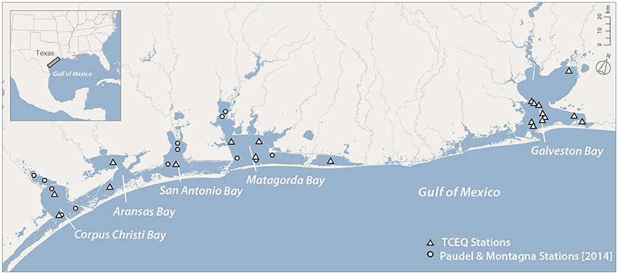
Figure 1. Texas estuaries and in situ data collection sites of the TCEQ and Paudel and Montagna (2014).

Study Area

Climate and Sedimentary Processes

Numerous shallow-water estuaries are found along the Texas coast (see Figure 1). These estuaries are drowned river valleys that formed during the Holocene after the last sea-level low stand. They are separated from the Gulf of Mexico by a thin chain of barrier islands and spits that span the length of the Texas Coast (Davis and FitzGerald, 2004; Davis, 2011). Small tidal inlets, the majority of which are jettied and dredged, connect the estuaries to the Gulf. These estuaries are in a microtidal (0.6 m Gulf and less than 0.3 m estuary tidal range), wave-dominated mixed energy coastal setting, and are affected by a climatic gradient with wetter conditions to the north and drier to the south (McKee and Baskaran, 1999; Davis, 2011; Montagna et al., 2011). For all bays, marine sediment input is thought to be relatively small due to the microtidal setting (Yeager et al., 2006). The bottom sediments and those in suspension mostly consist of fine-grained silt and clay (McKee and Baskaran, 1999). Average grain size for Texas bays range from 2.3 to 8 phi (Folger, 1972). For Corpus Christi Bay, the predominant bay bottom sediments range in grain size from 4.0 to 8.0 phi (Shideler, 1984). Average depths in Texas estuaries range from 2 to 4 m.

This case study focuses on the suspended sediment dynamics of Corpus Christi Bay (Figure 2). Corpus Christi Bay is about 284 km² and the deepest of the Texas bays with an average depth of 4 m (McKee and Baskaran, 1999). This estuary was chosen for comparison with a previous study by Shideler (1984). Relatively little freshwater enters this estuary from the Nueces River and Oso Creek. Low amounts of freshwater inflows coupled with high rates of evaporation cause the estuary to become hyper-saline for much of the year (Montagna et al., 2012).

FIGURE 2

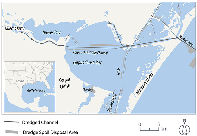
Figure 2. Detailed map of Corpus Christi Bay.

Wind along the Texas coast is prevalently from the southeast for the majority of the year (spring-summer) complemented by predominant northerlies (fall-winter). The prevalent southeasterlies are stronger in the south and decrease in speed moving northeastward along the coast. The wind is strongest during spring and progressively decreases in speed during the summer. In contrast, frontal passages, “northers” or winter storms, bring the dominant wind from the north with wind speed often greater than 15 m/s. During these frontal passages, northerly wind gusts are generally preceded by high southerly wind speeds (Ward, 1997). Shideler (1984) showed that wind-waves is the most important forcing of suspended sediments in Corpus Christi Bay.

Dredging and Related Impacts

Substantial modifications have occurred within Texas estuaries through the dredging of deep ship channels. In Corpus Christi Bay, the main channel is 14 m deep, spans the length of the estuary in an east-west direction and is maintained for navigation (Kraus, 2007). Other shallower dredged channels are scattered throughout these estuarine systems (Figure 2). In Corpus Christi Bay, the Intracoastal Waterway (ICW) bisects the eastern portion of the bay. Sediment from routine dredging for channel maintenance are placed in subaqueous disposal areas next to navigation channels. While active dredging operations suspend large amounts of sediment, the materials are typically contained in boomed-off areas resulting in small impacted areas relative to the size of the estuary. Dredging operations are conducted over short periods of time for up to a few months. A lasting effect of dredging, however, is the alteration of the Bay bathymetry through the creation of subaqueous disposal areas. Sediments of placement areas may have a higher propensity to be suspended by wind-wave action as less wave energy is needed to suspend these materials due to their shallower depth relative to the rest of the bay.

Datasets

The main data sets for this study consisted of two in situ data sets for the calibration and independent validation of the algorithm and MODIS satellite imagery processed to remove sun glint. The in situ suspended sediment data used to calibrate the study's model for transforming MODIS imagery to TSS was collected by the TCEQ. The TCEQ catalogs its surface water samples in the Surface Water Quality Monitoring Information System (SWQMIS) (Texas Commission on Environmental Quality, 2008). TCEQ in situ measurements are collected following the Total Suspended Solid (TSS) EPA STORET Standard Method 2450b. This measurement involves taking a volume of water from a point within an estuary and passing it through a pre-weighed glass fiber filter. The filter is then dried and weighed with the mass of the sample divided by the volume of water filtered, normally denoted in mg/l. These measurements are typically made quarterly, however, some sites in the dataset are sampled sporadically for special projects. Data were extracted from the SWQMIS (Texas Commission on Environmental Quality, 2008) for the period spanning 2002–2010. For this analysis, only TSS data collected from the primary and secondary bays (Figure 1) were used. If coincident sampling of CHL-α was present, this too was extracted. To avoid mixed land-water pixels in the MODIS data, TCEQ data were omitted if stations were within a kilometer of the shoreline. Measurements were also removed if they were located within or near Sabine Lake and any points south of Corpus Christi Bay. Sabine Lake data were removed because the CDOM-rich water coming from the Neches River may bias the optical signal. Areas south of Corpus Christi Bay were left out of the input dataset because the area is relatively shallow, and the possibility for bottom reflectance contaminating the TSS signal is high. As a result, a total of 704 in-situ samples were selected for inputs for model development.

Overflights from the polar-orbiting satellite Aqua carrying National Aeronautics and Space Administration's (NASA)'s Moderate-Resolution Imaging Spectroradiometer (MODIS) provide almost-daily images of estuaries and coastal areas. The MODIS sensor onboard NASA's Aqua satellite has been in orbit since 2002. MODIS was designed with 36 spectral channels to support observations of oceans, land, and clouds (McClain, 2009). There are nine 1-km bands designed for ocean color observations in the visible to near-infrared (NIR) (412–816 nm) portion of the electromagnetic spectrum. Over turbid waters of inland and coastal areas, however, the dynamic range of the sensor can be exceeded, leaving the actual signal to be unknown (Franz et al., 2006). Many researchers are now using the land/cloud bands to quantify suspended sediment concentrations in coastal waters (Matthews, 2011). The land (1 and 2) and cloud bands (3–9) have spatial resolutions of 250 and 500 m, respectively. These land/cloud bands are less sensitive than the 1-km ocean color bands, have broader dynamic ranges and do not suffer from the problems of the l-km resolution ocean color bands (Franz et al., 2006). Band 1 is optimal for detecting suspended sediment due to high reflectance from sediment in the water column around the red portion of the spectrum centered at 645 nm. Using the red portion of the spectrum, quantifying suspended sediments has little impact from phytoplankton pigments, such as CHL-α, in low concentrations (Bukata, 1995). Recently, MODIS land bands have been used to quantify suspended sediments in coastal estuaries with 250 and 500-m MODIS data (Doxaran et al., 2009; Feng et al., 2014).

The 500-m MODIS-Aqua Surface-Reflectance Product (MYD09GA) was chosen for use in this study because it includes atmospherically corrected bands 1–4, red, near infrared blue, and green, mostly used for ocean color applications and a cloud detection flag. The MYD09GA product is generated from MODIS Level 1B for land bands 1–7 and are estimates of surface spectral reflectance corrected for both atmospheric scattering and absorption (Vermote and Kotchenova, 2008). Doxaran et al. (2009) used the MYD09 and its counterpart MOD09 to quantify suspended sediments accurately in the Gironde estuary, France. Doxaran et al. (2009) developed an algorithm using a remote sensing reflectance (Rrs) ratio of Bands 1 and 2, red and near-infrared, respectively. In their study, they found that the atmospheric correction used by the land data community was sufficient to quantify suspended sediment concentration ranging from 77 to 2,182 g/m³. The combination of high spatial resolution, daily-repeat time, and a greater than 12-year data period, makes these land products ideal for creating an EDR of suspended sediments in estuaries and coastal water bodies.

Wind speed and direction data were extracted from the National Center for Environmental Prediction (NCEP) North American Regional Reanalysis model (NARR) (Mesinger et al., 2006). These data were used for creation of the wind roses and the implementation of the sun glint algorithm. Over water, significant areas of remotely-sensed satellite imagery can be contaminated with sun glint, a disk-like spot that has higher reflectance values than the surrounding area in the satellite imagery. Fresnel reflection causes sun glint and its magnitude is dependent on a combination of complex interactions of surface roughness of the water that is influenced by wind speed and direction, and solar and sensor viewing geometries (Zhang and Wang, 2010). MODIS data are routinely contaminated by sun glint because the satellite does not have a glint tilting avoidance strategy (Wang and Bailey, 2001). The MYD09GA data product does not include a glint coefficient because its use is for land applications; thus, Rrs data over water is sometimes contaminated by sun glint. We, therefore, implemented the sun glint algorithm created by Wang and Bailey (2001). Use of this algorithm allowed for the removal of contaminated Rrs data from inputs into algorithm development and the removal of contaminated data in the TSS EDR created for this study. Wind speed data were extracted from the NCEP NARR (Mesinger et al., 2006) for the locations and time of the MODIS image capture for input into the sun glint algorithm.

An independent dataset collected by Paudel and Montagna (2014) was used to validate the final TSS algorithm. These data were collected in Matagorda, San Antonio, and Corpus Christi Bays, and follow the same methods as the TCEQ SWQMIS. Sampling sites are spread over these estuaries and provide quarterly sampling from 2011 to 2013. In total, there were 137 cloud free data points that were available prior to sunglint filtering. Surface water samples for TSS and CHL-α were collected for every in situ location. Use of this independent dataset gave an impartial assessment of the final algorithm's accuracy and illustrated its robustness.

Methods

Model Development for Transforming Rrs to TSS

The TSS reflectance model was developed using in situ and remote sensing reflectance data derived from the MYD09GA data product. These data products were downloaded using NASA's Reverb data discovery tool (http://reverb.echo.nasa.gov/) for each day data were available in the SQWMIS database. From the 709 in-situ samples, a total of 294 unique days of satellite data were available. Satellite data collected from Reverb spanned from 8-13-2002 to thru 5-3-2010. NASA's SeaDAS 7.0.1 software was used to extract atmospherically corrected reflectance, viewing geometries, and flags from MYD09GA files over the SWQMIS collection sites when concurrent collections were within 4 h of the overflight of the satellite. Atmospherically corrected reflectance data were then multiplied by pi to derive Rrs data.

After data extraction was complete, MYD09GA data were combined with SQWMIS in situ data. To avoid the influence of bottom reflectance and algal absorption on Rrs data, individual TSS measurements were removed from the calibration data if (1) the collection depth was <3 m unless TSS values were greater than 50 mg/l, and (2) the sample's CHL-α values were greater than 30 mg/l following suggestions from Bukata (1995). To avoid sun glint and other interference, data were removed if (1) it was flagged as cloud reflectance in the MYD09 dataset, (2) sun glint coefficient was >0.001 (Wang and Bailey, 2001), and (3) sensor zenith angles were greater than or equal to 60 degrees. After these data had been filtered, 55 of the 704 data points remained for the development of the TSS model with TSS values ranging from 4 to 178 mg/l.

Spearman rank correlation coefficients were generated from Rrs Bands 1–4 and combinations of Rrs ratios between TSS to determine the best candidates for inputs into the model. Spearman correlation was used because it is less influenced by outliers and can show non-linear relationships among data (Wilks, 2011). Using the first three highest ranked correlation coefficients, linear and exponential regression models were fit to satellite and TSS data. Finally, the MYD09GA data over the in situ sites of Paudel and Montagna (2014) were extracted. The dataset was filtered following the same procedure as the calibration dataset with the difference that high CHL-α samples were not removed. This step was omitted as only one data point would have been excluded, and this portion of the data is used for validation only. The high CHL-α content collected in this sample shows how the algorithm is influenced in algal bloom conditions. After filtering had been applied to the validation set, 35 of the 137 data points were left in this validation dataset. The models' fit to the calibration dataset was quantified using the Root Mean Squared Error (RMSE) and the R-squared metrics. The validation dataset was used to quantify the Mean Absolute Error (MAE) and mean bias of the model.

TSS Time Series Development

The TSS reflectance model with the best performance was then applied to all available scenes of the MYD09GA land product over the study areas. These data were downloaded from https://lpdaac.usgs.gov/ and totaled 4,503 analyzed scenes for this study. Each image was then filtered for clouds, sun glint, and satellite geometries following the methodologies mentioned above, and daily cloud-free TSS maps were created at 500-m resolution. There was a maximum of 1,444 scenes of cloud free, glint free, and geometrically compatible imagery, however, on a pixel-by-pixel basis, this number varied due to the cloud mask and on average there were 1,226 scenes available for Corpus Christi Bay. Both individual scenes and composites were produced to show suspended sediment patterns in the estuaries (see Figure 5). Composite images were generated by computing medians and interquartile ranges (IQR) of satellite-derived TSS data for the entirety of the valid scenes of the satellite dataset. Seasonal comparisons were generated for Corpus Christi Bay for wind patterns to highlight the respective temporal variability, and show the different distributions and patterns of TSS for the different time periods. Here satellite data within 1 km of land are removed to avoid mixed pixels of land and water. Also, to avoid data contamination from bottom reflectance, any data occurring in water shallower than 1 m was removed.

Seasonal Wind Analysis

To investigate wind-wave resuspension, wind speed data at 10 m height for the study period were extracted from the NCEP NARR model (Mesinger et al., 2006) over Corpus Christi Bay. The NARR's 32-km spatial and 3-h temporal resolutions were considered sufficient for this analysis. Wind data were analyzed to determine seasonal patterns. Data were split into seasonal wind regimes, and wind roses were plotted and compared to TSS composites for each regime. The period of November—February is characterized by frontal passages and dominant northerly winds and is referred to as the frontal passages period. The March–June period is characterized by weaker fronts at the beginning of the period and prevalent southeasterlies, and is referred to as the southeasterly period. The last period of July–October is also characterized by prevalent southeasterlies, however, their magnitude is lower when compared to the southeasterly period and referred to as the quiet period (quiet period). Wind data were then plotted as wind roses for each regime. Composites of satellite-derived TSS patterns are compared to the related wind rose plots for the three identified wind regimes in Figure 6 to determine if the wind speed and directional component influences the sediment distributions in the estuary.

Results and Discussion

TSS Model Results and Discussion

Spearman rank correlations identified the highest correlations between individual bands and band ratios with the TSS data collected by the TCEQ. The correlation analysis found that Rrs 645, Rrs 645/Rrs 555, and Rrs 645/Rrs 469 had the highest correlations with TSS, at 0.65, 0.79, and 0.63, respectively. These radiometric values were then fit to derive TSS using linear and exponential models. In total there were six models tested three linear and three exponential (Table 1). A comparison of the empirical models tested to derive TSS from Rrs and Rrs ratios are presented in Table 1 along with their fit statistics. The model with lowest MAE of validation dataset was selected to create the TSS EDR. As indicated in Table 1, the best model was an exponential function using the band reflectance ratio of Rrs 645/ Rrs 555. The equation for this algorithm is:

$\begin{array}{ll}y=a^{*}{e}^{b*x}& (1)\end{array}$

Where y is the estimate for TSS in mg/l and x is the Rrs 645/Rrs 555 reflectance ratio from the MYD09GA dataset. Coefficients a and b and their 95% confidence intervals were 1.696 (0.703, 2.689) and 3.562 (3.030, 4.094), respectively. The model fits quite well to the data with an R-square of 0.81 and RMSE of 16.1 (n = 55) for the TCEQ calibration data (Figure 3). The MAE for the validation dataset is 17.52 (n = 35) with a mean bias of −13.40. Model fit to the data is illustrated in Figure 3. The uncertainty in this model is estimated to be 13% according to the RMSE compared to the range of the calibrated data. It is interesting to note that the model underestimates 66% of the validation dataset, however, these values still fall with the 95% confidence interval of the model fit. While exact cause of the bias is unknown, potential reasons for the bias include radiometer drift and slight differences in TSS processing. The model was fit to data spanning 2003 to 2010 and validation data was collected from 2011 to 2013, a drift in the satellite radiometer could account for this difference. Slight differences in the TSS sampling methods may also account for the differences.

TABLE 1

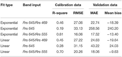
Table 1. Model fit statistics for calibration dataset and validation dataset error metrics for linear and exponential models for estimating TSS from Rrs and Rrs band ratios.

FIGURE 3

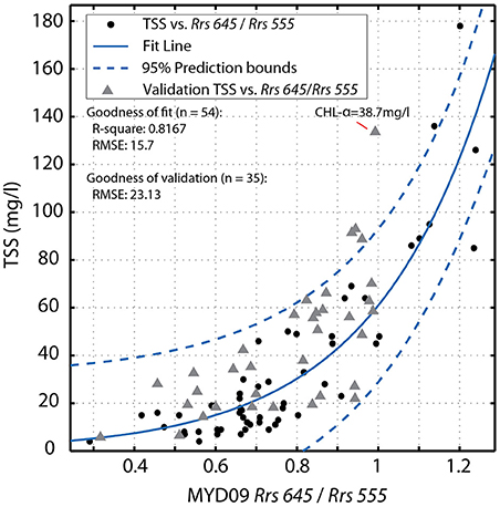
Figure 3. Model produced by Equation 1 for the estimation of TSS from MYD09 reflectance with in situ data collected by TCEQ (black circles) and validation dataset (gray triangles) collected by Paudel and Montagna (2014).

In order to gain more confidence in this model high concentration TSS measurements are needed in both the calibration and validation dataset to achieve a more robust quantification of error. While this model performs well over a range of TSS values in several Texas estuaries, more validation data is needed to quantify the true error of the model. Individual models tuned for individual estuaries may reduce the error using the same method, but this was not possible due to an insufficient number of in situ data points within each estuary.

Usage of this algorithm for deriving TSS from Rrs will cause over- and under-estimations of TSS in high concentrations of CDOM and CHL-α, respectively. An example is included in the validation data set where a high concentrations of CHL-α causes the algorithm to underestimate the true concentration of sediment in the water (Figure 3). The TSS value of 133.7 mg/l in the validation data set occurred during an algal bloom with a CHL-α density of 38.4 mg/l. For this case, the modeled TSS was 59.8 mg/l, which underestimates the actual measurement by 73.9 mg/l. While this is a large error, algal blooms in these estuarine waters are infrequent events. To further illustrate CHL-α influence on the model a sensitivity analysis was conducted on CHL-α vs. modeled TSS residuals for both the calibration and validation datasets (Figure 4). We found no systematic influence of CHL-α on predicted TSS values, except for the aforementioned high concentration sample of CHL-α. For the majority of the year, the suspended sediments in these Texas estuaries are mostly composed of suspended inorganic particles (McKee and Baskaran, 1999). Thus, the influence of algal blooms will only impact the EDR created from this algorithm for a small percentage of the time allowing for analysis of suspended sediment dynamics in Texas estuaries. The influence of CDOM on the algorithm could not be quantified because neither TCEQ nor Paudel and Montagna (2014) collected such measurements. With these limitations, this algorithm shows promise in creating a TSS EDR for Texas estuaries.

FIGURE 4

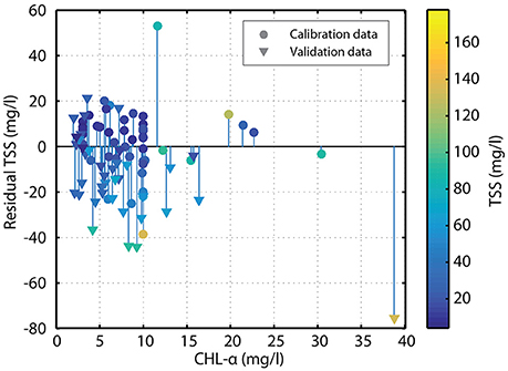
Figure 4. Residual TSS from TSS model plotted against CHL-a sampled concurrently for both the calibration (triangles) and validation dataset (circles). Calibration and validation datasets are colored based on in situ TSS-values.

Development of this model enables the creation of synoptic suspended sediment maps in Texas estuaries. Figure 5 compares a MODIS-Aqua true color image with estimated TSS concentrations for the same scene, the Texas estuaries and coast, following the passage of a cold front. The largest TSS concentrations along the coast are observed for Galveston Bay and Matagorda Bay.

FIGURE 5

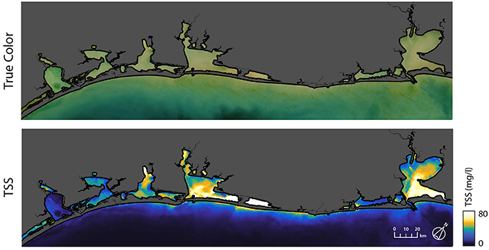
Figure 5. MODIS-Aqua 500-m True Color RGB image and example of output from TSS algorithm for same scene following the passage of a cold front on January 10th 2006.

TSS Patterns and Forcings for Corpus Christi Bay

TSS composites and wind roses for Corpus Christi Bay are presented in Figure 6. During the frontal passages period, median, and IQR TSS are higher in the southern portion of the estuary, windward of the predominant north-northeast wind direction. Median TSS and IQR values increase as the fetch lengths increase. The similar patterns of both IQR and median TSS with values increasing with fetch length and highest on the windward side of the estuary suggest that wind-wave resuspension from frontal passages is the dominant process controlling suspended sediment concentrations during this period. These patterns are similar to those reported by Shideler (1984) during the same wind regime. TSS median values are the lowest during this period when compared to other wind regimes in this estuary, possibly resulting from the combination of low wind speeds between frontal passages and a relatively low frequency of such events. The majority of wind speeds during this period are <7.5 m/s (Figure 6) while there are typically 10 frontal passages during the frontal passages period (Ward, 1997). Low wind speeds between frontal passages are likely not significant enough to generate waves that impart sufficient bed shear stress for resuspension as the bay is 4 m deep on average, the deepest along the Texas coast. Another area that exhibits a behavior similar to the southern portion of the estuary during the same period are the dredge spoil deposition sites along the ICW (Figure 6). Elevated median TSS and higher IQR values compared to the rest of the bay occur at these locations. Yet these areas fetch lengths are considerably smaller in the direction of the prevalent wind. These areas have more unconsolidated dredged sediments and are shallower than the rest of the estuary thus sediments are more readily suspended.

FIGURE 6

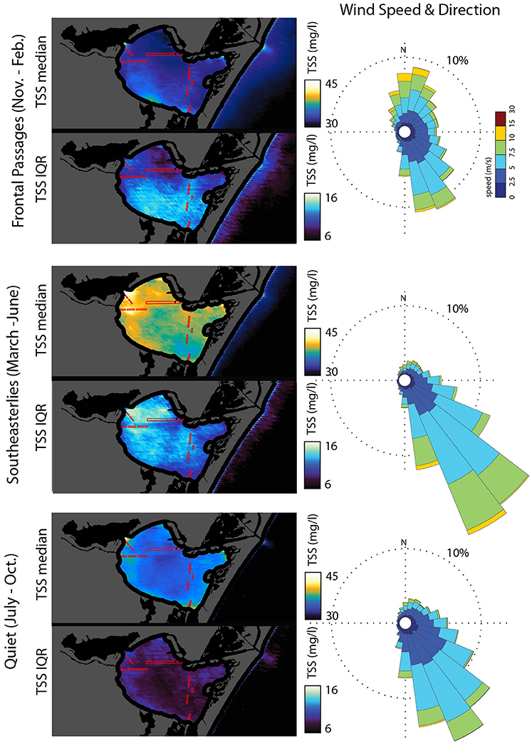
Figure 6. Corpus Christi Bay TSS Median and IQR with corresponding wind rose for each wind regime. Red rectangular polygons are dredge spoil deposition sites.

Another factor that may influence the measured patterns is bias due to cloud presence (Eleveld et al., 2014). Higher wind periods may be under represented compared to the actual resuspension events that occur because the majority of cold fronts are accompanied by cloud-cover that obscures the satellites view of the estuary. The frontal passages period composites of Corpus Christi Bay support Shideler's (1984) hypothesis that Nueces Bay is a fluvial sediment storage basin having a control valve activated by strong northerly wind. Suspended sediments are released into Corpus Christi Bay during frontal passages as indicated by the higher median and IQR TSS values near the entrance to Nueces Bay. These higher TSS values compared to those of the surrounding area are consistent with suspended sediments spilling into Corpus Christi Bay when strong wind is blowing for a prolonged period from the north.

The influence of tides is more difficult to identify using the composite patterns, however, some observations can be made. Lower IQR values are observed along the length of the Corpus Christi Ship Channel (Figure 6). Additionally, median and IQR values are lower than surrounding values at the entrance of the Corpus Christi Ship Channel into the main portion of the bay. Both observations are consistent with flood plumes that are lower in suspended sediment concentration originating in the Gulf of Mexico. These lower values indicate that, for Corpus Christi Bay, inflow of Gulf waters reduces the concentration of sediment within and surrounding the ship channel but not for the bay at large. Export of suspended sediments from the Bay to the Gulf of Mexico is evident from an ebb plume at the exit of the ship channel into the Gulf of Mexico for all wind regimes with the largest plumes observed for the frontal passages period (Figure 6). Higher TSS concentrations are observed along the shorelines of the Gulf of Mexico for the frontal passages period as compared to the other wind regimes consistent with strong offshore northerly winds often accompanying frontal passages. It is hypothesized that wave action generated by the southerly winds preceding frontal passages results in resuspension of nearshore sediments and that offshore northerly winds then transport the suspended sediments further offshore.

The southeasterly period has the highest concentrations of median and IQR TSS values. Similar to the frontal passages period, both Median and IQR TSS values increase along fetch length in the dominant wind direction. Highest median and IQR TSS values are located along and near the windward shore in the northwestern quadrant of Corpus Christi Bay. This area is where the predominant and prevalent wind of this wind regime has the longest fetch lengths, ~18 km. Similarly to the frontal passages period, this pattern indicates that wind-wave resuspension is the dominant process influencing estuarine suspended sediment distribution during this period. The median TSS composite resembles the pattern in Shideler's (1984) southeasterly mode. Similar to Shideler's (1984) observations, the southeastern quadrant of Corpus Christi Bay has very low concentrations of TSS. These low TSS concentrations are attributed to a flux of sediment free waters from the Upper Laguna Madre being pushed into the southern portion of Corpus Christi Bay by the southeasterly wind.

Dredge spoil placement sites exhibit similar behavior to those during the frontal passages period. The dredge spoil area located on the ICW has higher median and IQR TSS values than the surrounding area (Figure 6). These higher values during both the frontal passages period and southeasterly period illustrate that these areas are more prone to wind-wave resuspension. The dredge spoil site next to the entrance of the port of Corpus Christi also has higher median and IQR values than those of the surrounding area.

During the quiet period (Figure 6), the Corpus Christi Bay median and IQR values are relatively uniform. Areas near and along the windward shore have slightly elevated values when compared to the rest of Corpus Christi Bay. The low concentrations of median and IQR TSS values are compatible with a wave dominated TSS with less sediment than during any of the other time periods. The IQR pattern also displays the lowest values indicating consistently low TSS concentrations during the quiet period. The highest concentrations of median TSS values are located over the dredge spoil deposition area near the Port of Corpus Christi similar to during the southeasterly period.

Potential Limitations of the Study

It is important to note that the seasonal median TSS composites may be biased by cloud presence obscuring satellite view of estuaries and thus providing lower representation of scenes associated with frontal passages, southeasterlies, sea breeze, and thunderstorms. While these biases likely influence total estimated suspended sediment concentrations, the overall seasonal changes in resuspended sediment concentration patterns are unlikely to be substantially affected by these biases and are still clearly identifiable permitting assessment of the importance of the respective forcing mechanisms.

Another potential limitation of this study is the influence that CDOM and high CHL-α have on the reflectance ratio algorithm. Areas with high CDOM concentrations cause overestimates of TSS concentrations while areas of high CHL-α cause underestimates of TSS concentrations. This bias is believed to be minimal for Corpus Christi Bay.

Conclusions

A TSS algorithm was created to quantify suspended sediment in estuaries of the Texas Coast based on MODIS reflectance data and a comparison with two in situ data sets collected in the study area during the period 2002–2014. The algorithm includes filtering of the data for geometries, sun glint, and water depth, and an exponential function that gives the best fit for TSS concentrations ranging from 4 to 176 mg/l. After calibration based on a long-term TCEQ data set, the algorithm was further validated with an independent data set, acquired outside of the model's calibration period. However, we did find that the algorithm does not provide accurate results for cases with CHL-α values greater than 30 mg/l. Future users of the model and TSS EDR generated for this study should be aware of this and other limitations of the method.

The model was applied to create an EDR of suspended sediments for Corpus Christi Bay. Analysis of the EDR reveals that the bay is influenced by wind-wave resuspension with different patterns during the predominant northerlies and prevalent southeasterlies seasons. The impact of dredging is apparent in long-term TSS patterns as concentrations of suspended sediments over dredge spoil disposal sites are higher and more variable than surrounding areas, which is most likely due to their less consolidated nature and shallower depths requiring less wave energy for sediment resuspension. This study highlights the advantage of how long-synoptic time series of TSS can be used to elucidate the major drivers of suspended sediments in estuaries.

Author Contributions

AR wrote the article, collected field data, developed algorithm, and performed analysis. PT aided in algorithm development, analysis of data, and writing of article. JG aided in algorithm development, analysis of data, and editing of text.

Funding

This study was supported by grant number NA09NMF4720179 from the National Oceanic and Atmospheric Administration under the Comparative Assessment of Marine Ecosystem (CAMEO) program, and National Aeronautics and Space Administration Headquarters under the NASA Earth and Space Science Fellowship Program—Grant NNX12AO09H. Partial support was also provided by the Harte Research Institute for Gulf of Mexico Studies at Texas A&M University-Corpus Christi. The funders had no role in study design, data collection and analysis, decision to publish, or preparation of the manuscript.

Conflict of Interest Statement

The authors declare that the research was conducted in the absence of any commercial or financial relationships that could be construed as a potential conflict of interest.

Acknowledgments

The authors would like to thank the reviewers, Sachidananda Mishtra and Matthew Lewis for their helpful and constructive comments that greatly contributed to improving the final version of the paper.

References

Bukata, R. P. (ed.). (1995). Optical Properties and Remote Sensing of Inland and Coastal Waters. Boca Raton, FL: CRC Press.

Google Scholar

Chen, Z., Hu, C., Muller-Karger, F. E., and Luther, M. E. (2010). Short-term variability of suspended sediment and phytoplankton in Tampa Bay, Florida: observations from a coastal oceanographic tower and ocean color satellites. Estuar. Coast. Shelf Sci. 89, 62–72. doi: 10.1016/j.ecss.2010.05.014

CrossRef Full Text | Google Scholar

D'sa, E. J., and Miller, R. L. (2005). “Bio-optical properties of coastal waters,” in Remote Sensing of Coastal Aquatic Environments, eds R. L. Miller, C. E. Del Castillo, and B. A. Mckee (Dordrecht: Springer), 129–155.

PubMed Abstract | Google Scholar

Davis, R. A. (2011). Sea-Level Change in the Gulf of Mexico. College Station: Texas A&M University Press.

Google Scholar

Davis, R. A., and FitzGerald, D. M. (2004). Beaches and Coasts. Oxford: Blackwell Publ.

Google Scholar

Doxaran, D., Froidefond, J. M., Castaing, P., and Babin, M. (2009). Dynamics of the turbidity maximum zone in a macrotidal estuary (the Gironde, France): observations from field and MODIS satellite data. Estuar. Coast. Shelf Sci. 81, 321–332. doi: 10.1016/j.ecss.2008.11.013

CrossRef Full Text | Google Scholar

Eleveld, M. A., van der Wal, D., and van Kessel, T. (2014). Estuarine suspended particulate matter concentrations from sun-synchronous satellite remote sensing: tidal and meteorological effects and biases. Remote Sens. Environ. 143, 204–215. doi: 10.1016/j.rse.2013.12.019

CrossRef Full Text | Google Scholar

Feng, L., Hu, C., Chen, X., and Song, Q. (2014). Influence of the three Gorges Dam on total suspended matters in the Yangtze Estuary and its adjacent coastal waters: observations from MODIS. Remote Sens. Environ. 140, 779–788. doi: 10.1016/j.rse.2013.10.002

CrossRef Full Text | Google Scholar

Folger, D. W. (1972). Characteristics of Estuarine Sediments of the United States. U.S. Govt. Print. Off. Available online at: https://pubs.er.usgs.gov/publication/pp742742 (Accessed November 20, 2016).

Franz, B. A., Werdell, P. J., Meister, G., Kwiatkowska, E. J., Bailey, S. W., Ahmad, Z., et al. (2006). “MODIS land bands for ocean remote sensing applications,” in Proceedings of Ocean Optics XVIII (Montreal, QB).

Google Scholar

Green, M. O., and Coco, G. (2014). Review of wave-driven sediment resuspension and transport in estuaries. Rev. Geophys. 52, 77–117. doi: 10.1002/2013RG000437

CrossRef Full Text | Google Scholar

Kraus, N. C. (2007). “Coastal inlets of Texas, USA,” in Coastal Sediments'07, eds N. C. Kraus and J. D. Rosanti (Reston, VA: American Society of Civil Engineers), 1475–1488.

Google Scholar

Matthews, M. W. (2011). A current review of empirical procedures of remote sensing in inland and near-coastal transitional waters. Int. J. Remote Sens. 32, 6855–6899. doi: 10.1080/01431161.2010.512947

CrossRef Full Text | Google Scholar

McClain, C. R. (2009). A decade of satellite ocean color observations*. Annu. Rev. Mar. Sci. 1, 19–42. doi: 10.1146/annurev.marine.010908.163650

PubMed Abstract | CrossRef Full Text | Google Scholar

McKee, B. A., and Baskaran, M. (1999). “Sedimentary processes of Gulf of Mexico Estuaries,” in Biogeochemistry of Gulf Mexico Estuaries, eds T. S. Bianchi, J. R. Pennock, and R. R. Twilley (New York, NY: Wiley), 63–85.

Google Scholar

Mesinger, F., DiMego, G., Kalnay, E., Mitchell, K., Shafran, P. C., Ebisuzaki, W., et al. (2006). North American regional reanalysis. Bull. Am. Meteorol. Soc. 87, 343–360. doi: 10.1175/BAMS-87-3-343

CrossRef Full Text | Google Scholar

Miller, R. L., and McKee, B. A. (2004). Using MODIS Terra 250 m imagery to map concentrations of total suspended matter in coastal waters. Remote Sens. Environ. 93, 259–266. doi: 10.1016/j.rse.2004.07.012

CrossRef Full Text | Google Scholar

Montagna, P. A., Brenner, J., Gibeaut, J., and Morehead, S. (2011). “Coastal impacts,” in The Impact of Global Warming on Texas, eds J. Schmandt, J. Clarkson, and G. R. North (Austin: University of Texas Press), 97–123.

Google Scholar

Montagna, P., Palmer, T. A., and Pollack, J. (2012). Hydrological Changes and Estuarine Dynamics. New York, NY: Springer Science & Business Media.

Google Scholar

Paudel, B., and Montagna, P. A. (2014). Modeling inorganic nutrient distributions among hydrologic gradients using multivariate approaches. Ecol. Inform. 24, 35–46. doi: 10.1016/j.ecoinf.2014.06.003

CrossRef Full Text | Google Scholar

Petus, C., Chust, G., Gohin, F., Doxaran, D., Froidefond, J.-M., and Sagarminaga, Y. (2010). Estimating turbidity and total suspended matter in the Adour River plume (South Bay of Biscay) using MODIS 250-m imagery. Cont. Shelf Res. 30, 379–392. doi: 10.1016/j.csr.2009.12.007

CrossRef Full Text | Google Scholar

Ruhl, C. A., Schoellhamer, D. H., Stumpf, R. P., and Lindsay, C. L. (2001). Combined use of remote sensing and continuous monitoring to analyse the variability of suspended-sediment concentrations in San Francisco Bay, California. Estuar. Coast. Shelf Sci. 53, 801–812. doi: 10.1006/ecss.2000.0730

CrossRef Full Text | Google Scholar

Shideler, G. L. (1984). Suspended sediment responses in a wind-dominated estuary of the Texas Gulf Coast. J. Sediment. Res. 54, 731–745.

Google Scholar

Stumpf, R. P., and Pennock, J. R. (1989). Calibration of a general optical equation for remote sensing of suspended sediments in a moderately turbid estuary. J. Geophys. Res. 94:14363. doi: 10.1029/JC094iC10p14363

CrossRef Full Text | Google Scholar

Texas Commission on Environmental Quality (2008). TCEQ Surface Water Quality Monitoring Procedures Volume 1: Physical and Chemical Monitoring Methods for Water, 202.

Vermote, E. F., and Kotchenova, S. Y. (2008). MOD09 (Surface Reflectance) User's Guide, Version 1.1, March, 2008. Greenbelt, MD.

Google Scholar

Wang, M., and Bailey, S. W. (2001). Correction of sun glint contamination on the SeaWiFS ocean and atmosphere products. Appl. Opt. 40, 4790–4798. doi: 10.1364/AO.40.004790

PubMed Abstract | CrossRef Full Text | Google Scholar

Ward, G. H. (1997). Processes and Trends of Circulation within the Corpus Christi Bay National Estuary Program Study Area. Corpus Christi, TX: Corpus Christi Bay National Estuary Program.

Google Scholar

Ward, G., and Montague, C. (1996). Estuaries. New York, NY: McGraw-Hill Book Company.

Google Scholar

Wilks, D. S. (2011). Statistical Methods in the Atmospheric Sciences. Oxford: Academic press.

Google Scholar

Yeager, K. M., Santschi, P. H., Schindler, K. J., Andres, M. J., and Weaver, E. A. (2006). The relative importance of terrestrial versus marine sediment sources to the Nueces-Corpus Christi Estuary, Texas: an isotopic approach. Estuar. Coasts 29, 443–454. doi: 10.1007/BF02784992

CrossRef Full Text | Google Scholar

Zawada, D. G., Hu, C., Clayton, T., Chen, Z., Brock, J. C., and Muller-Karger, F. E. (2007). Remote sensing of particle backscattering in Chesapeake Bay: a 6-year SeaWiFS retrospective view. Estuar. Coast. Shelf Sci. 73, 792–806. doi: 10.1016/j.ecss.2007.03.005

CrossRef Full Text | Google Scholar

Zhang, H., and Wang, M. (2010). Evaluation of sun glint models using MODIS measurements. J. Quant. Spectrosc. Radiat. Transf. 111, 492–506. doi: 10.1016/j.jqsrt.2009.10.001

CrossRef Full Text | Google Scholar